Discussion Papers Statistics Norway Research department No. 801 February 2015

Marina Rybalka

The innovative input mix Assessing the importance of R&D and ICT investments for firm performance in manufacturing and services

•

Discussion Papers No. 801, February 2015 Statistics Norway, Research Department

Marina Rybalka The innovative input mix Assessing the importance of R&D and ICT investments for firm performance in manufacturing and services

Abstract: Business innovation is an important driver of productivity growth. In this paper, I assess the importance of R&D and ICT investment for firm performance in the manufacturing and service industries. Explicitly, I use an extended version of the CDM model that treats ICT together with R&D as the main inputs into innovation and productivity, and test it on a large unbalanced panel data set based on the innovation survey for Norway. Four different types of innovation and the number of patent applications are used as innovation output measures. I find that ICT investment is strongly associated with all types of innovation in both sectors, with the result being strongest for product innovation in manufacturing and for process innovation in service industries. The impact of ICT on patenting is only positive in manufacturing. Overall, ICT seems to be less important than R&D for innovation, but more important for productivity. These results support the proposition that ICT is an important driver of productivity growth. Given the high rate of ICT diffusion in Norway, my results also contribute to explaining what is referred to as the ‘Norwegian productivity puzzle’, i.e. the fact that Norway is one of the most productive economies in the OECD despite having relatively low R&D intensity. Keywords: Innovation, ICT, R&D, Productivity, CDM model, Manufacturing and Services JEL classification: D24, L60, L80, O3 Acknowledgements: I am grateful to Erik Biørn, Ådne Cappelen, Jarle Møen, Arvid Raknerud and Terje Skjerpen for interesting discussions and many helpful comments. This paper was written as part of the research project ‘Effects of ICT on firm innovation and productivity’ with financial support from the Norwegian Ministry of Local Government and Modernisation. Address: Marina Rybalka, Statistics Norway, Research Department. E-mail: [email protected]

Discussion Papers

comprise research papers intended for international journals or books. A preprint of a Discussion Paper may be longer and more elaborate than a standard journal article, as it may include intermediate calculations and background material etc.

© Statistics Norway Abstracts with downloadable Discussion Papers in PDF are available on the Internet: http://www.ssb.no/en/forskning/discussion-papers http://ideas.repec.org/s/ssb/dispap.html ISSN 1892-753X (electronic)

Sammendrag I OECDs rapport om norsk økonomisk utvikling (OECD, 2007) fremheves det såkalte norske paradokset: at Norge har en meget lav satsing på FoU i forhold til andre høyinntektsland, men likevel en av de høyeste per kapita-inntektene i verden, et av de høyeste produktivitetsnivåer i industrien, og en av de høyeste levestandarder. Rapporten viser også at skårene på ulike innovasjonsindikatorer for Norge ligger klart lavere enn gjennomsnittet for andre OECD-land. Det har blitt gjennomført flere studier for å belyse det norske produktivitetsparadokset (se for eksempel OECD, 2008; Castellacci, 2008; og nylig Asheim, 2012 og von Brasch, 2015). Disse studiene trekker frem følgende mulige forklaringer på paradokset: (i) landets næringsstruktur med den høye produktiviteten i råvarebasert industri; (ii) det at Norge har en av Europas høyeste andeler av personer med høyere utdanning; og (iii) det at innovasjonsindikatorer måles for snevert og FoU investeringer ofte underrapporteres av norske foretak. Ingen av studiene nevner at Norge er et av de landene som har ligget lengst fremme når det gjelder intensiv bruk av Informasjons- og kommunikasjonsteknologi (IKT) og spredning av bredbåndsteknologi. I 2011 var også Norge ledende i elektronisk handel blant OECD-land (kilde: www.oecd.org, Key ICT Indicators). Samtidig viser flere empiriske studier på foretaksnivå (for eksempel, Bresnahan mfl., 2002; Brynjolfsson og Hitt, 2003 og Hempell, 2005) at IKT-investeringer bidrar til økt produktivitetsvekst, særlig når det utføres komplementære investeringer rettet mot organisasjonsmessige endringer og prosessinnovasjoner. Halvorsen (2006), som studerer produktivitetsutviklingen i norsk økonomi for perioden 1981–2003, finner at TFP-veksten i private tjenesteytende næringer var mye høyere på 1990-tallet enn på 1980-tallet. Den sterke veksten fortsatte i 2001–2003. Von Brasch (2015) viser videre at den sterkeste TFP-veksten i årene 1978–2007 har skjedd innenfor Varehandel, samtidig som Rybalka (2009) viser at foretakene i Varehandel var blant de mest kapitalintensive når det gjelder IKT-kapital i årene 2002–2006. Gitt at teknologisk utvikling er en av de sentrale faktorene bak den beregnede TFP-veksten, gir alle disse tallene en støtte for velkjente oppfatninger om at moderne løsninger innenfor distribusjon og bruk av IKT aktivt har bidratt til å endre produksjonsprosessene og ført til produktivitetsvekst i denne næringen og som følge av det i den norske økonomien som helhet. I den foreliggende studien åpner jeg for at IKT sammen med FoU og høykvalifisert arbeidskraft er sentrale forklaringsfaktorer både for innovasjon og produktivitet. Mer presist ser jeg på hvilken effekt IKT-investeringer har på foretakenes tilbøyelighet til innovasjoner i form av nye produkter, prosesser, organisasjonsmessige endringer og nye markedsføringsmetoder, samt deres utvikling mht. patentsøkning og arbeidsproduktivitet. Dette gjør jeg ved å bruke data fra Innovasjonsundersøkelsene i perioden 2004–2010 i kombinasjon med en utvidet versjon av CDM-modellen (Crepon mfl., 1998, Polder mfl., 2009 og Hall mfl., 2013). Studien inneholder også en sammenlignende analyse av betydningen av IKT for innovasjonsresultater og produktivitet i industri og tjenesteytende næringer. Jeg finner at IKT investeringer per ansatt har en klart signifikant effekt på tilbøyeligheten til alle typer innovasjoner. Den sterkeste effekten er på produktinnovasjon i industri og prosessinnovasjon i tjenesteytende næringer. Kun for industrien finner jeg en positiv sammenheng mellom IKT og antall patenter som foretaket har søkt om. Også arbeidskraftens sammensetning, målt ved andelen ansatte med høy utdanning, gjør foretaket mer innovativt og produktivt, alt annet likt. Foretakets IKTkapitalintensitet spiller også en positiv rolle for produktiviteten og effekten er betydelig sterkere for produktivitet enn for innovasjon. Dette resultatet viser at IKT er en viktig faktor bak produktivitetsvekst og at høye norske IKT-investeringer bidrar betydelig til å forklare det såkalte norske paradokset.

3

1. Introduction Business innovation is regarded as a potentially important driver of productivity growth, both at the firm and the national level. At the micro level, business innovation has the potential to increase consumer demand through improved product or service quality and simultaneously decrease production costs. At the macro level, strong business innovation increases multifactor productivity, thus increasing international competitiveness, economic growth and real per capital incomes.1 It is therefore of great interest to businesses and policy-makers to identify the factors that stimulate innovation and to understand how these factors interact. R&D is an important factor behind innovations, but it is not the only one. Today, firms invest in a wide range of intangible assets, such as data, software, patents, new organisational processes and firm-specific skills. Together, these nonphysical assets make up a firm’s knowledge-based capital, KBC (see OECD, 2013). A lack of proper control for intangible assets and underinvestment in KBC are seen as the main candidates for explaining the poor productivity performance of European countries relative to the USA.2 The need for Europe to move into the knowledge-based economy and support investment in KBC has been an important focus of government policy in European countries (see OECD, 2013).

Recently, more and more attention has been devoted to the role of Information and Communication Technology (ICT) as an enabler of innovation (see, for instance, Vincenzo, 2011). ICT is one of the most dynamic areas of investment, as well as a very pervasive technology.3 The possible benefits of ICT use to a firm include among others increased input efficiency, general cost reductions and greater flexibility in the production process. This technology can also stimulate innovation activity in a firm, leading to higher product quality and the creation of new products or services. Its use has the potential to increase innovation by improving possibilities for communication and speeding up the diffusion of information through networks. For example, technologies that allow staff to effectively communicate and collaborate across wider geographic areas will encourage strategies for less centralised management, leading to organisational innovation. Previous analyses confirm that ICT plays an important role in firm performance, e.g. Brynjolfsson and Hitt (2000, 2003), OECD (2004), Gago and Rubalcaba (2007), Crespi et al. (2007) and van Leeuwen (2008). These studies evaluate the effects of

1

See, for instance, Crépon et al. (1998), Griffith et al. (2006) and Parisi et al. (2006) for the studies at the micro level, and van Leeuwen and Klomp (2006) for the study at the macro level. 2 See, for instance, van Ark et al. ( 2003), O’Sullivan (2006), Moncada-Paternò-Castello et al. (2009), Hall and Mairesse (2009) and Hall et al. (2013). 3

ICT is often referred to as a modern general purpose technology, GPT (see Bresnahan and Trajtenberg, 1995, for a definition of GPT, and Castilione, 2012, for an investigation of GPT features of ICT).

4

ICT use and innovation on productivity. A few recent studies, i.e. Hall et al. (2013), Vincenzo (2011) and Polder et al. (2009), focus on the direct link between ICT and innovation.

One aim of the current study is to assess the effects of ICT as an enabler of innovation in Norwegian firms and to assess its relative importance for innovation and productivity compared to R&D. Do effects differ for different types of innovations? Four types of innovations are under investigation: a new (or improved) product, a new (or improved) production process, an organisational innovation and a new marketing method. I also use a count of patent applications as an alternative measure of innovative activity in firms. Figure 1. Share of firms with access to broadband in 2004 or 2003 (bars) and in 2011 (  ). Firms with 10 or more employees

Iceland (2003)

Greece

Italy

Slovak Republic

Poland

Ireland

Czech Republic

EU27

Luxembourg

Portugal

France (2003)

United Kingdom

Germany

Netherlands

Austria

Norway

Slovenia

Sweden (2003)

Estonia

Belgium

Finland

Spain

Denmark

100 90 80 70 60 50 40 30 20 10 0

Source: www.oecd.org, Key ICT Indicators

Another aim of the study is to investigate whether a high level of ICT diffusion in Norway could explain the so-called ‘Norwegian puzzle’, i.e. the fact that, while R&D spending in the Norwegian business sector as a share of GDP is below the OECD average, the productivity performance of Norwegian firms is among the strongest in the OECD (see OECD, 2007). Several studies endeavour to explain the ‘Norwegian puzzle’ (also referred to as the Norwegian productivity paradox). OECD (2008) points to the skill level of the adult population and financial support from the public sector as positive factors behind Norway’s strong productivity performance. On the other hand, they find weak innovation activity in the manufacturing sector. Castellacci (2008) claims that the source of the Norwegian productivity paradox lies in the sectoral composition of the economy. Recently, Asheim (2012) discussed the lack of registration of all inputs and outputs in innovation activities and points to underreporting of R&D investments and innovation activities in the national R&D statistics. While 5

providing several possible explanations for the ‘Norwegian puzzle’, none of these studies mention the high level of diffusion of ICT in Norway. For example, 60.3 per cent of Norwegian firms had access to broadband already in 2004, while the average for EU27 at that time was 46.5 per cent (see Figure 1). Also in 2011, when most European firms had access to broadband (the average for EU27 was 89.2 per cent), Norway was one of the leading European countries in e-commerce (see Figure 2 and OECD, 2011). This fact is one of the reasons why the current paper directs the attention to data on Norwegian firms. What is the relative importance of ICT for productivity compared to other key inputs, such as R&D and human capital, in a country with a high rate of ICT diffusion? Are they complements or substitutes? Figure 2. Internet selling and purchasing1 in all industries in 2011 (2010 when indicated, * 2010 only for purchasing). Firms with 10 or more employees

1

Most countries explicitly use the OECD concept of internet commerce, that is, goods or services that are ordered over the internet, but where payment and/or delivery may be off line. Source: www.oecd.org, Key ICT Indicators

To investigate these research questions, I apply the currently most used model for analysing the link between innovation input, innovation output and productivity, the so-called CDM model (Crepon et al., 1998). The standard version of the CDM model is a structural model that studies the following 6

interrelated stages of the innovation chain: the choice by a firm of whether or not to engage in R&D; the amount of resources it decides to invest in R&D; the effects of these R&D investments on innovation output; and the impact of innovation output on the productivity of the firm. In the spirit of Polder et al. (2009) and Hall et al. (2013), I rely in this paper on an extended version of the CDM model, which treats ICT investment together with R&D as two main inputs into innovation and productivity. While Hall et al. (2013) base their study on manufacturing firms alone, Polder et al. (2009) compare manufacturing firms with firms in services. Such comparison seems to be of substantial importance.

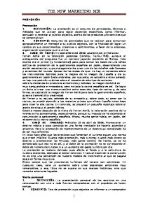
If we check the development of total factor productivity (TFP) in different industries in Norway in the three last decades compared to the USA,4 we will see that most changes have taken place in the Wholesale and retail trade sector (see Figure 3). While the productivity level in the manufacturing sector remained between 60 and 70 per cent below the corresponding productivity level in the USA during the period 1978–2007, the Wholesale and retail trade sector showed a great increase in relative TFP, and, by 2007, it had almost reached the US level. At the same time, the Wholesale and Retail trade industries (when studied at the more detailed industry level) are among the most ICT capitalintensive industries in Norway (see Table 3 in Rybalka, 2009), i.e. the average share of ICT capital services in total capital services in 2002–2006 was 26.8 per cent for the Wholesale and 17.4 per cent for the Retail trade (the corresponding share for manufacturing is just 5.7 per cent).5 Hence, it is very important to account for industry heterogeneity when studying the effects of ICT. In order to account for such heterogeneity, I present results for manufacturing firms and firms in services separately (in addition to the analysis of the whole economy). Keeping in mind the explanations of the ‘Norwegian puzzle’ in previous studies, I also take into account the skill level of employees in Norwegian firms when analysing the effects of R&D and ICT on innovation and productivity.

Beyond presenting results for the Norwegian economy, this paper contributes to the existing literature in several ways. Firstly, I take into account the pervasiveness of ICT and treat it in parallel with R&D as a main input into innovation, rather than simply as an input into the production function. Secondly, in order to account for industry heterogeneity, I provide separate results for manufacturing firms and firms in services (in addition to analysing the whole economy). Thirdly, I include marketing innovation in the analysis in addition to earlier investigated product, process and organisational

4

Since US productivity has grown faster than productivity in Europe, the USA is often used as a reference country when studying productivity development in European countries, see, e.g., van Ark et al. (2003) and Aghion et al. (2009). 5 This measure of ICT capital services is constructed on the basis of information about firms’ investments in hardware and software collected by Statistics Norway since 2002 (for details of the construction procedure, see Rybalka, 2009).

7

innovation. All four types of innovation are equally represented in the data, which makes it possible to analyse the whole set of innovation types and enables a better understanding of the innovation process in the firm. Finally, I use the number of patent applications as an alternative measure for innovation. While the combination of different innovation types shows the variety of innovative processes in a firm, the number of patent applications reflects the quality of the innovation, i.e. only the best innovative products are expected to be protected by patent. Figure 3. TFP levels in Manufacturing and the Wholesale and retail trade from 1978–2007 in some European countries relative to the US industry equivalents1

1

All monetary measures for different countries are calculated in 1997 prices and USD using industry-specific Purchasing Power Parities from EU-KLEMS data (for details, see von Brasch, 2015). Source: von Brasch (2015) based on OECD and EU-KLEMS data

For the analysis, I use a rich firm-level data set based on the four recent waves of the Community Innovation Survey (CIS) for Norway (CIS2004, CIS2006, CIS2008 and CIS2010), which contains information on different firms’ innovative activities. By supplementing these data with information on the number of patent applications from the Norwegian patent database and on ICT investment and other relevant information from different registers, I obtain an unbalanced panel of 14 533 observations of 8 554 firms. The estimation results indicate considerable differences between firms in manufacturing and service industries with respect to innovation and the productivity effects of R&D and ICT. While ICT investment is strongly associated with all types of innovation in both sectors, with the result being strongest for product innovation in manufacturing and for process innovation in service industries, the impact of ICT on patenting is only positive in manufacturing. The estimation results also confirm that R&D and ICT are both strongly associated with innovation and productivity, with R&D investment being more important for innovation, and ICT investment being more important for productivity. These results suggest that ICT is an important driver of productivity growth that, together with human capital, should be taken into account when trying to explain the ‘Norwegian productivity puzzle’.

8

The paper is organised as follows. Section 2 summarises the main findings from previous studies and explains the extended version of the CDM model. Section 3 presents the data set, the main variables and some descriptive evidence. Section 4 discusses the estimation of the empirical model, and Section 5 presents the results. Finally, Section 6 concludes.

2. Theoretical framework 2.1 ICT and firm performance Several previous analyses confirm that ICT plays an important role in business success. One of the first attempts to quantify the role of ICT assets in firm performance in the form of productivity was made by Brynjolfsson and Hitt (1995). Since then, a broad range of empirical studies has emerged exploring the impacts of ICT on firm performance.6 Most of these studies employ a production function framework to estimate the elasticity of output with respect to ICT capital, controlling for other factors, including innovations. However, very few of them focus on the direct link between ICT use and innovation.

As Koellinger (2005) puts it, ‘ICT makes it possible to reduce transaction costs, improve business processes, facilitate coordination with suppliers, fragment processes along the value chain (both horizontally and vertically) and across different geographical locations, and increase diversification’. Each of these efficiency gains provides an opportunity for innovation. For example, technologies that allow staff to communicate effectively and collaborate across wider geographic areas will encourage strategies for less centralised management, leading to organisational innovation.

ICT also enables closer links between businesses, their suppliers, customers, competitors and collaborative partners, which are all potential creators of ideas for innovation (see Rogers, 2004). By enabling closer communication and collaboration, ICT helps businesses to be more responsive to innovation. For example, having broadband internet, a web presence and automated system linkages helps businesses to keep up with customer trends, monitor competitors’ actions and get rapid user feedback, thereby helping them to exploit opportunities for all types of innovations. Gretton et al. (2004) suggest the following two reasons why businesses’ use of ICT encourages innovative activity. Firstly, ICT is a ‘general purpose technology’ that provides an ‘indispensable

6

See, for example, studies by Atrostic and Nguyen (2002), Biscourp et al. (2002), Bresnahan et al. (2002), Brynjolfsson and Hitt (2003), Crespi et al. (2007), Hall et al. (2013), Hempell (2005) and OECD (2004).

9

platform’ upon which further productivity-enhancing changes, such as product and process innovations, can be based. For example, a business that establishes a web presence sets the groundwork from which process innovations, such as electronic ordering and delivery, can be easily developed. In this way, adopting general purpose ICT makes it relatively easier and cheaper for businesses to develop innovations. Secondly, the spill-over effects from ICT use, such as network economies, can be sources of productivity gains. For example, staff of businesses that have adopted broadband internet are able to collaborate more closely with wider networks of academics and international researchers on the development of innovations.

A lack of proper control for intangible assets and the differences in industrial structure, specifically the smaller ICT producing sector, are seen as the main candidates for explaining the differences in productivity growth that are observed between Europe and the USA (for a comparative analysis of productivity growth in Europe and the USA, see, e.g., van Ark et al., 2003; O’Sullivan, 2006; Moncada-Paternò-Castello et al., 2009; and Hall and Mairesse, 2009). It is also true that firms’ total R&D and ICT investments measured as shares of GDP are lower in Europe than in the United States and that the ICT gap is somewhat larger than that for R&D (see Figure 1 in Hall et al., 2013). Hall et al. (2013) report so high rates of return on both ICT and R&D investments for Italian firms that they suspect considerable underinvestment in both these activities.

Another line of literature investigates the importance of ICT for firms’ organisation (see Brynjolfsson and Hitt, 2000, for a survey and Bloom et al., 2009, for a recent study). Case studies show that the introduction of information technology is combined with a transformation of the firm, investment in intangible assets, and changes in relations with suppliers and customers. Electronic procurement, for instance, increases the control of inventories and decreases the costs of coordinating with suppliers, and ICT offers the possibility of flexible production: just-in-time inventory management, integration of sales with production planning etc.

The available microeconometric evidence shows that a combination of investment in ICT and changes in organisations and work practices facilitated by these technologies contributes to firms’ productivity growth. For instance, Crespi et al. (2007) use Innovation survey data for the UK and find a positive effect on firm performance of the interaction between ICT and organisational innovation. Gago and Rubalcaba (2007) find that businesses that invest in ICT, particularly those that regard their investment as strategically important, are significantly more likely to engage in services innovation. Van Leeuwen (2008) shows that e-sales and broadband use significantly affect productivity through

10

their effect on innovation output. However, broadband use only has a direct effect on productivity if R&D is not considered as an input to innovation. This approach is further developed by Polder et al. (2009). Their study finds that ICT investment is important for all types of innovation in services, while it plays a limited role in manufacturing, being only marginally significant for organisational innovation. Cerquera and Klein (2008), in contrast, find that more intense use of ICT brings about a reduction in R&D efforts in German firms. The results for nine OECD countries in Vincenzo (2011) are consistent with ICT having a positive impact on firm innovation activity, in particular on marketing innovation and on innovations in services. However, there is no evidence that ICT-intensive firms have greater capacity to introduce ‘more innovative’ (new-to-the-market) products, suggesting that ICT enables the adoption of innovation rather than the development of new products. For Italian manufacturing firms, Hall et al. (2013) find that ICT investment intensity is associated with product and organisational innovation, but not with process innovation, although not having any ICT investment is strongly negative for process innovation. These few recent papers, which investigate R&D and ICT investment jointly, have produced conflicting results as regards the impact of ICT on innovation. In addition, very few papers have investigated these effects separately for manufacturing and services. Hence, more evidence is needed.

2.2 Modelling framework The currently most used model for analysing the link between innovation input, innovation output and productivity is called the CDM model (Crepon et al., 1998). It was applied, for instance, in Lööf and Heshmati (2002), Parisi et al. (2006) and van Leeuwen and Klomp (2006). The standard version of the model contains three different blocks: (1) First, the firm decides whether or not to invest in R&D; and how much to invest, if it chooses to do so; (2) second, the innovative input leads to the innovative output (e.g. product or process innovation, new technology, organisational change); (3) finally, the innovative output leads to increased labour productivity. Several recent studies have modified the standard CDM model in order to include other factors than R&D in the knowledge production function. For example, Castellacci (2011) uses the CDM model to investigate the effects of industrylevel competition on firms’ innovation and productivity for Norway, while ICT is implemented in the CDM model by Griffith et al. (2006) for four European countries (France, Germany, Spain and the UK), Polder et al. (2009) for the Netherlands and by Hall et al. (2013) for Italy. These extensions of the standard model specification lead to extra difficulties in the estimation of the model, owing to the increased number of equations with qualitative dependent variables, for instance, when using different

11

innovation types as a measure of innovative output. However, it is possible to bypass some of these difficulties by estimating the different blocks of the model sequentially.7 In this paper, I follow Polder et al. (2009) and Hall et al. (2013) and use an extension of the standard CDM model that analyses the effects of ICT on different stages of the innovative process. This version of the extended CDM model is presented in Figure 4. While Polder et al. (2009) use ICT as an additional input in the knowledge production function, but not in the production function, in Hall et al. (2013), the ICT investment is an input both in the production function and in the knowledge production function. While the former is in line with the more traditional view that ICT leads to productivity gains (e.g. through implementing new work practices and, hence, cost reductions and/or improved output); the latter introduces a less traditional view, i.e. that ICT may also stimulate innovation activity in the firm by speeding up the diffusion of information, promoting networking among firms, enabling closer links between businesses and customers, and leading to the creation of new goods and services. Consequently, this modelling framework treats ICT as a pervasive input rather than as an input in the production function only. In this paper, I apply the model extension used in Hall et al. (2013). A more detailed description of different blocks of the model follows below.

Figure 4. CDM model augmented with ICT

7

Note that this estimation strategy requires bootstrapping of standard errors, which I provide for some of the models.

12

Block 1: R&D input decision This block does not differ from the first part of the standard CDM model. It models firm i’s decision to engage in R&D activities in period t. First the firm decides whether or not to start to invest in R&D in the given period; if it decides to invest, the firm then sets the amount of R&D investments. This statement of the problem can be modelled with a standard sample selection model (see Heckman, 1979): (1)

1 if rdit*  xitrd1  eit  c rdit   , 0 else

where rd it is the observed binary endogenous variable equal to zero for non-R&D and one for R&Dperforming firms, rd it* is a corresponding latent variable that expresses some decision criterion, such that a firm decides to invests in R&D if rd it* is above a certain threshold c, xitrd is a vector of firm characteristics (e.g. size, age, international orientation etc., and a constant term), 1 is the associated coefficient vector, and eit is an error term. Once a firm has decided to engage in R&D activities, it must set the amount of resources devoted to R&D investments. Analogous to the previous equation and in line with the standard formulation of the CDM model, the latent R&D intensity of a firm i in a given period t, rit* , is represented as a function of another set of firm characteristics, xitr : (2)

rit*  xitr 2   it ,

where  2 is the associated coefficient vector, and  it is an error term. The observed R&D intensity, r, is then equal to:

(3)

r * if rdit  1 rit   it 0 else

The pair of random disturbances eit and  it is assumed to be jointly i.i.d. normally distributed, with zero mean and covariance matrix given by

(4)

 1    ,  2       

13

where  e and   are the standard errors of eit and  it ,  e  1 by standardisation, and  is their correlation coefficient. This model can be estimated by maximum likelihood. Block 2: Innovation output Let us now consider a model of how innovation occurs. R&D efforts lead to innovation output. Let

INNO * be a latent variable that measures the extent of creativity/research activity within the firm. The higher the value of INNO * , the higher is the probability that an innovation will occur. This modelling framework is influenced by Griliches (1990), Crepon et al. (1998) and Parisi et al. (2006). The main idea in this literature is that, by investing in R&D, the firm accumulates a knowledge capital stock, which plays an important role in its innovation activities. An extended version of the CDM model also includes an ICT intensity, ict, together with R&D intensity, r, in the knowledge production function: (5) where

INNOit*  1  rit   2  ictit  xitinno   it

xitinno is a vector of different firm characteristics important for innovation output (e.g. firm size,

industry, cooperation in R&D projects etc., and a constant term), 1 ,  2 and  are parameters (vectors) of interest, and it is an error term.

The previous empirical studies based on the CDM model use different innovation output measures to proxy unobserved knowledge, INNOit* , e.g. the share of innovative sales (applied, for example, in Crepon et al., 1998, and Castellacci, 2011); different binary innovation indicators (applied, for example, in Griffith et al., 2006, for product and process innovation; in Polder et al., 2009, for product, process and organisational innovation; and in Hall et al., 2013, for product, process and two types of organisational innovation); and patent applications counts (applied, for example, in Crepon et

al., 1998). In this paper, I estimate equations for the following measures of innovation output in the second model block: (i) the probability of any innovation; (ii) the probability of four different types of innovation (product, process, organisational and marketing innovation); and (iii) the expected number of patent applications. In the first case, an equation for the binary indicator of any innovation is estimated as a probit model. In the second case, a system of four equations for binary indicators of corresponding types of innovation is estimated as a quadrivariate probit model, accounting for the mutual dependence of the error terms. In the latter case, since numbers of patent applications are observed as integer numbers with many zero observations, they are modelled by zero-inflated count

14

data model (see Chapter 18.4.8 in Greene, 2011, for a description of the model and Aghion et al., 2009, for the application of the zero-inflated count data model to the patent data).8 Note that the variables for R&D intensity, r, and ICT intensity, ict, are endogenous because these investments are simultaneously determined with innovation activities. I discuss this issue in more detail under empirical model estimation in Section 4. Block 3: Production function The final block of the CDM model focuses on the effects of innovation output on labour productivity. In order to incorporate a firm’s ICTs in the last block of the standard CDM model, I follow Hempell (2005) and use a traditional Cobb-Douglas production function with labour and two types of capital as inputs: (6)

Yit  Ait K it  1 ICTK it  2 Lit  3 .

In (6), Yit is the output of firm i in period t, measured as value added in constant prices, Kit and ICTKit are the corresponding amounts of tangible and ICT capital inputs in constant prices, Lit is the labour input, and Ait is total factor productivity (TFP). The parameters  1 ,  2 and  3 correspond, respectively, to output elasticities of the two types of capital and labour, and TFP is assumed to be determined by: (7)

ln( Ait )   0  INNOit1  xitp 2   it .

p In (7), INNOit is a vector of innovation output variables and xit is a vector of different firm

characteristics important for productivity (for instance, firm size, age and location);  0 ,  1 and  2 are parameters (vectors) of interest and  it is a white noise error term that comprises measurement errors and firm-specific productivity shocks. Dividing by Lit and taking logarithms on both sides of (6) yields: (8)

 lpit   0   1 kit   2 ictkit   3lit  INNOit  1  xitp 2   it ,

8

In this model, the zero outcomes can arise from one of two regimes, i.e. in one regime the outcome is always zero, and in the other, the usual count data generating process applies. Then, in the first step, the inflation equation that models the probability of falling in regime one is estimated by probit, and, in the second step, the standard count data generating process is estimated conditional on the outcome of the first step of estimation. I use a binary indicator for any type of innovation as a main inflate variable, since I expect that only innovative firms can apply for a patent. In addition, the inflation equation includes firm age, industry and location, and time dummies.

15



where  3  ( 1   2   3  1) and the small letters lp, l, k and ictk denote the logarithm of labour productivity, Y/L, labour input, L, tangible capital intensity, K/L, and ICT capital intensity, ICTK/L, correspondingly.9

I also allow for heterogeneous labour input. Both economic theory and empirical evidence suggest that there is a key link between the skill level of the workforce and economic performance. Hence, omitting heterogeneity in the quality of labour may lead to overstating the productivity of ICT capital and innovation output. To account for this bias, I decompose a firm’s workforce into employees who are high-skilled (with at least 13 years of education) and low-skilled (with less than 13 years of education).10 Letting Nh and Nl denote the corresponding amounts of man-hours (where the total amount of man-hours N= Nh +Nl) and θ denote the productivity differential of high-skilled workers compared to low-skilled workers, effective labour input Lit is specified as:

Lit  N l ,it  (1   ) N h ,it  N it (1   hit ) ,

(9)

where hit  N h ,it / N it denotes the share of hours worked by high-skilled workers in the firm. Taking the logarithm of (9) and inserting the expression for lit into (8) yields:

(10)

 lpit   0   1 kit   2 ictkit   3 nit   4 hit  INNOit  1  xitp  2   it , 

where the approximation follows from ln(1   hit )   hit and  4   3 .11 The inclusion of skill shares in the production function specification as in (10) in order to control for heterogeneity of labour quality is a common approach in the literature (see, for example, Lehr and Lichtenberg, 1999, Caroli and van Reenen, 1999, Bresnahan et al., 2002, and Hempell, 2005). I use OLS for the estimation of this block of the model.

9

Note that I do not impose constant return to scale, whereas ICT is allowed to affect productivity both directly (through the ICT capital variable) and indirectly (through the innovation output variable). The latter extension of the standard CDM model requires the use of exclusion restriction(s) or the non-linear functional form for identification of the total effect of ICT on productivity. I do use the non-linear functional form for identification of the model and I have some variables that are included in the vector of firm characteristics xitinno in the innovation equation and not in the vector xitp in the productivity

equation. However, as I will discuss in more detail in Section 4, I cannot really claim to find causal effects of R&D and ICT on innovation and productivity. Therefore, all reported results in the paper should be viewed as representing associations rather than causal relationships. 10 This number of years of education corresponds to completed upper secondary education or vocational training. 11 The first–order Taylor approximation is quite accurate if the values of θ and h are not too large. Anticipating some of the results and applying mean shares for h, the implicit product θh=0.05 is small enough for the approximation to work well (for values 0)c ICT investors (ICT>0)c 89.3% 92.8% 86.1% R&D investment intensitya,b,d 108.0 112.7 73.6 23.6 26.7 20.5 ICT investment intensitya,b,d Firms with at least one innovationc 47.9% 100% Firms with product innovationc 28.8% 60.1% Firms with process innovationc 21.5% 44.8% Firms with organisational innovationc 21.6% 45.1% Firms with marketing innovationc 25.8% 53.8% Firms with at least one patentc 10.1% 18.4% 2.4% Number of patent applicationsb,e 2.1 2.2 1.2 a Units are NOK thousands in real terms (base year = 2001) per employee. b Mean values. c Share of observations with corresponding firm characteristic. d Calculated for the sample of firms with positive investment. e Calculated for the sample of firms with at least one patent application.

21

(4) Obs. on manufacturing firms (N=6199) 561.4 91.3 19.5 0.021 0.074 19.7% 63.6% 42.6% 36.5% 12.7% 8.2% 21.3% 22.4% 19.6% 38.9% 88.9% 68.2 14.8 55.0% 35.8% 25.6% 23.7% 29.8% 14.5% 2.3

(5) Obs. on firms in services (N=6145) 685.3 93.0 16.2 0.053 0.049 43.8% 62.0% 49.7% 36.7% 7.5% 6.1% 15.0% 15.5% 9.9% 29.0% 90.3% 165.8 36.3 48.8% 29.7% 21.6% 21.6% 27.3% 8.2% 1.8

Relatively few Norwegian firms have an international orientation, i.e. only 15 per cent of the firms sell their main products or services on the international market (Europe and rest of the world), while more than half of the firms (about 52 per cent) sell their main products or services on the local or regional market, and about 33 per cent operate at the national level. More than 60 per cent of the observations concern firms that belong to a group. The same high shares are observed by Castellacci (2011) for Norwegian CIS data and by Polder et al. (2009) for Dutch CIS data (compared to just 25 per cent of Italian manufacturing firms in Hall et al., 2013). That could be the result of the over-representation of medium-sized and large firms in Norwegian CIS data (these firms are often part of a group), i.e. firm size distribution is skewed to the right, with an average of 92, but with a median of only 30 employees (see Table A2). Approximately 17 per cent have cooperated on innovation, either with a university/college/research institute or with another firm, while approximately 13 per cent of the firms purchased R&D services from an external provider. Only 16 per cent of firms in my final sample are R&D subsidy recipients, in contrast to Hall et al. (2013), where 42 per cent of the firms receive subsidies (however, their subsidy variable comprises subsidies both for R&D and for other types of investments).

Turning to the innovation output variables, all four types of innovation are well-represented in the data, the shares of observations varying between 21 and 29 per cent (see column 1 in Table 2). As for the combinations of different types of innovation, product innovation only (combination [1,0,0,0]), followed by all types of innovation (combination [1,1,1,1]), marketing innovation only (combination [0,0,0,1]) and organisational innovation only (combination [0,0,1,0]) are the most common innovation combinations among the innovative firms (see the observed frequencies for 16 combinations of four innovation types in Table C5). Not surprisingly, the distribution of the number of patent applications is extremely skewed to the right, with 90 per cent of observations being equal to zero and 80 per cent of those that applied for a patent being equal to one patent application (see Figure 5). Such a distribution of the number of patent applications can be captured by the zero-inflated count data models (see, e.g., Chapter 18 in Greene, 2011). This class of models takes into account that zero counts can arise from one of two regimes, i.e. in one regime, the outcome is always zero (in my case, if a firm does not innovate), and, in the other, the usual count data generating process applies (some innovative firms apply for a patent and some do not).

22

1173

250

Frequency 500 750

1000

1250

Figure 5. Distribution of number of patent applications (with N=13066 for zero patent applications and N=8 for more than 35 patent applications)

129

0

45

20 1515 11 6 10 3 4

0

5

10

3 6 2 3 3 1 1

1 1 2 1

15 20 25 Number of patent applications

1

30

1

1 1

35

Columns (2) and (3) in Table 2 present a comparison of the main firm-specific characteristics of innovative and non-innovative firms (the former are defined as those that have introduced at least one type of innovation in the survey period). The comparison shows a remarkable difference between the two groups, which is in line with the previous CDM analyses based on firm-level data for other countries (see, for example, Crepon et al., 1998; and Hall and Mairesse, 2006). On average, innovative firms are much bigger in size, have a higher share of high-skilled employees, an international orientation and a higher probability of belonging to a group than non-innovative firms. They are also more capital intensive. However, the former group is only slightly more productive. About 55 per cent of innovative firms and only 7 per cent of non-innovative firms are R&D performing firms, which supports the fact that R&D is an important input for innovation output. While approximately 18 per cent of innovative firms have applied for at least one patent, 2 per cent of non-innovative firms also have at least one patent application in the patent database. The latter observation is possible if some of the non-innovative firms have applied for a patent for an innovation introduced during the previous three-year period.17

17

These numbers support my intuitive choice of a binary indicator for any type of innovation as a main inflate variable when estimating the probability of outcome (the number of patent applications) to be zero or nonzero, i.e. the innovators have much higher probability to apply for a patent than non-innovators.

23

Finally, columns (4) and (5) in Table 2 present a comparison of the main firm-specific characteristics of manufacturing firms (NACE 15-36 in SN2002) and firms in service industries (NACE 51-74 in SN2002). We can observe a remarkable difference between these two groups. Being on average almost of the same size and slightly younger, firms in service industries are more productive, have a higher share of high-skilled man-hours and are much more ICT capital-intensive (although much less tangible capital intensive). Given that Business-related services (NACE 72-74) and Wholesale (NACE 51) were the most ICT capital-intensive industries in Norway in 2002–2006 (see Table 3 in Rybalka, 2009) and that these industries account for about 75 per cent of observations for the firms in service industries in the final sample (see Table A1), the latter observation is not surprising. At the same time, the firms in the service industries represented are less likely to have their main market abroad, and they also cooperate less on innovative activities, purchase R&D from external providers less often, and receive R&D funding less often. Not surprisingly, their innovative output is lower on average, both when proxied by different innovation types and by the number of patent applications. Interestingly, while there are fewer R&D investors among firms in service industries, those that do invest in R&D invest on average more intensively than R&D investors in manufacturing. One can also observe that the rate of ICT diffusion is high in both sectors (the shares of ICT investing firms are 88.9 and 90.3 per cent, respectively). However, firms in service industries invest more intensively in ICT. Thus, compared to manufacturing firms, firms in service industries appear to be younger, more domestically oriented, and rely relatively more on ICT and skilled labour. Although less innovative, they are, however, more productive.

4. Econometric model specification and estimation issues This section presents the econometric model specification for the extended version of the CDM model presented in Section 2. Econometric specification of block 1: R&D input decision This block is the same for all model specifications. It models an R&D input decision by firm i in time t and contains two R&D equations corresponding to the theoretical model (1)–(4): (1´)

rdit*  xitrd 1  eit ,

(2´)

rit*  xitr 2   it .

24

Econometric specification of block 2: Innovation output I use two proxies for innovation output when estimating the second model block based on equation (5), i.e. the probability of innovating and the number of patent applications. The probability of innovating can be estimated for any innovation (basic model) and for each of four different types of innovation (product, process, organisational and marketing innovation). The innovation equation when innovation output is proxied by any type of innovation is: (3a´)

innoit*  10  rit*   20  ictit   30  hit  xitinno  0  it0 .

The system of equations for the probability of the different types of innovation is:

(3b´)

 pdtit*  *  pcsit  * org it  mkt *  it

 11  rit*   21  ictit   31  hit  xitinno  1  it1  12  rit*   22  ictit   32  hit  xitinno  2  it2  13  rit*   23  ictit   33  hit  xitinno  3  it3

.

 14  rit*   24  ictit   34  hit  xitinno  4  it4

I model the probability of applying for a patent as a function of the binary indicator for any type of innovation, as well as firm age, industry and location, and time dummies. The patent equation is then specified as an expected number of patent counts for the firms that have positive probability of applying for a patent, sumpatit* , conditional on R&D intensity, r, ICT intensity, ict, and other variables equal to:

(3c´)

E ( sumpatit | rit* , ictit , hit , xitinno )  exp(15  rit*   25  ictit   35  hit  xitinno  5 ) .

Econometric specification of block 3: Productivity The econometric specification of the productivity equation based on the theoretical model (6)–(10) is: (4´)

 lpit   0   1 k it   2 ictk it   3 Lit   4 hit  INNOit* 1 + xitp  2   it ,

where INNO* is either the predicted probability of any innovation, or the set of dummies for the different combinations of innovation types: [1,1,1,1], [1,1,1,0], [1,1,0,1] etc. (with combination [0,0,0,0] as the reference category), or the expected number of patent applications per employee.18

18 Note that, to simplify the interpretation of the results, I use the predicted values for the number of patent applications divided by the number of employees in the firm as an explanatory variable in the productivity equation (such as k and ictk, which are the conventional and ICT capital per employee).

25

This empirical model is a recursive nonlinear system of equations, each of which focuses on one of the steps in the innovation process. The first equation models the probability that a firm with characteristics xitrd engages in R&D activities. It is estimated for the whole sample of firms. The second equation focuses only on firms with positive R&D investment, R >0, and studies how the R&D intensity of the firm, rit* , is affected by a set of firm characteristics xitr . The third equation analyses the link between two main innovation inputs (R&D and ICT), on the one hand, and innovation output (either any innovation, four different types of innovation, or the number of patent applications), on the other.19 Finally, the fourth equation estimates the effects of innovation output together with ICT capital on the labour productivity of the firm ( lpit ). When estimating the second and third model blocks, I also explore the influence of skill composition on the firm ( hit ), together with firm characteristics xitinno and xitp , correspondingly. Table 3 describes different firm characteristics that are comprised by the vectors xitrd , xitr , xitinno and xitp (marked by x) and other explanatory variables used in the estimation of equations (1´)–(4´). The choice of explanatory variables, such as Market location, Part of a group, Received subsidy and

Cooperation on innovation is inspired by both Hall et al. (2013) and Polder et al. (2009). However, I also include the Cooperation on innovation (at the national, Scandinavian, European or world level) and Purchased R&D variables in the Innovation output equation. This choice is based on the results in Cappelen et al. (2012), who show that firms collaborating with others on their R&D efforts are more likely to be successful in their innovation activities and patenting.20 Following Castellacci (2011), who estimates the CDM model based on Norwegian data, I also include Hampering factors (high costs, lack of qualified personnel and lack of information) in the estimation of the R&D choice model block 1. As Castellacci (2011) demonstrates, these factors are highly relevant for shaping the innovative process and are also valid instruments for handling the endogeneity problem of the R&D intensity variable when using it in the innovation output equation. While Hall et al. (2013) only control for the skill composition of the firm in the innovation output equation, I follow the standard CDM model in Crepon et al. (1998) and control for the skill composition of the workforce (share of high-skilled man19 The innovation equation (3a´) is estimated as a probit model. Equation (3b´) is a system of four equations with binary indicators of corresponding types of innovations. It is estimated as a quadrivariate probit model using the GHK (GewekeHajivassiliou-Keane) simulation algorithm (see Chapter 15 in Greene, 2011; and Cappellari and Jenkins, 2003), assuming the mutual dependence of the error terms. Finally, equation (3c´) is estimated as a zero-inflated negative binomial count data model by pseudo maximum likelihood. 20 At the same time, Cappelen et al. (2012) demonstrate that getting an R&D tax credit has a marginal effect on innovation (they only find a positive and significant effect for process innovation) and no effect on patenting. Hence, I choose not to control for receiving an R&D subsidy in the innovation output equation (in line with Hall et al., 2013, and Polder et al., 2009).

26

hours) also in the productivity equation. Further, I provide robustness checks for inclusion of that variable in the innovation output and productivity equations.

Table 3. Variables and methods used in the estimation of different model equations

Dependent variable: Explanatory variables: Employment (log) Employment squared (log) Positive R&D historya Market locationb Part of a groupb Hampering factorsb Received subsidyb Cooperation on innovationc Purchased R&Dc R&D intensity (log)d Share of high-skilled ICT intensity (log)e Tangible capital intensity (log)e Innovation outputd Age dummies Industry dummies Regional dummies Time dummies

Estimation method:

Eq. (1´)

Eq. (2´)

Dummy for R>0

log(R&D spending per employee)

x x x x x x

x x x x x x x

x x x yes

x x x yes

Maximum likelihood (ML) by Heckman procedure

Notes: Different firm characteristics that are comprised by the vectors

Eq. (3´) Eq. (4´) Any innovation/ four types of log(VA per innovation / employee) number of patent appl. x x

x x r* h ict

x x x yes ML for probit / GKH simulation for quadrivariate probit / pseudo ML for zeroinflated count data

x x

h ictk k INNO* x x x yes

OLS

xitrd , xitr , xitinno and xitp are marked by x.

a

Exclusion restriction when estimating (1´) and (2´) by Heckman procedure. Used to instrument the R&D intensity variable, r*, when estimating (2´) and using predictions for r* in (3´). c Used to instrument the innovation output variable, INNO*, when estimating (3´) and using predictions for INNO* in (4´). d Predicted from the previous estimation stage. e Set to zero when the corresponding investment is zero and dummies for such observations are included. b

Identification Several important econometric issues arise in the estimation of this type of CDM model. The first is the possible sample selection bias due to the fact that only a fraction of the firm population innovates, whereas a large number of firms in the sample are not engaged in R&D activities at all (only 30 per cent of the observations in the final sample have positive R&D values). In addition, the firms may have some kind of innovative effort, but it is not always reported (see Griffith et al., 2006) and some

27

firms may underestimate their R&D (e.g. when it is performed by workers in an informal way).21 In line with the previous CDM empirical studies, I correct for the selection bias by estimating (1´) and (2´) as a system of equations by maximum likelihood, assuming that the error terms in (1´) and (2´) are bivariate normal with zero mean and covariance matrix as specified in equation (4). In the literature, this model is often referred to as a Heckman selection model (see Heckman, 1979) or type II Tobit model (see Amemiya, 1984). For identification of such a model, the vector xitrd in equation (1´) should contain at least one variable that is not in the vector xitr in equation (2´). Nevertheless, all previous works in the CDM literature use the same explanatory variables in both equations. The main reason for this practice is that it is difficult to find the factors explaining a firm’s likelihood of engaging in R&D that are not related to the amount of resources the firm decides to invest in R&D. In addition to identification ‘by functional form’, I use a dummy variable for the firm’s previous R&D investments (whether a firm had any R&D activity in the previous 3 years) as an exclusion restriction. On the one hand, I believe that firms that have previous R&D experience have a higher probability of engaging in R&D activities in the given period. On the other hand, it is not obvious that having R&D experience implies higher R&D intensity in the given period (it can happen that ‘new’ R&D investors, or firms that took a break from investing in R&D, invest more intensively in R&D in the given period than firms that invest continuously).22 I elaborate more on the selectivity issues and check for the appropriate choice of explanatory variables and of an ‘exclusion restriction’, as well as the sensitivity of the results to that choice, in Section 5 when estimating the model.

The second econometric issue refers to the endogeneity of some of the main explanatory variables. Since (1´)–(4´) is a system of recursive equations, it is natural to assume that the main explanatory variable in Equation (4´) (innovation output) is endogenously determined in the previous innovation stage, i.e. in innovation equation (3´); in turn, the main explanatory variable in Equation (3´) (innovation input) is determined in the previous innovation stage, i.e. the R&D intensity equation (2´). The standard CDM model handles this problem of the R&D intensity endogeneity by predicting R&D intensity, rit* , from the estimates of the first block of the model (R&D input decision) and using it as an explanatory variable in the innovation equation (3´). Similarly, to handle the endogeneity of the

21 Asheim (2012) points to underreporting of R&D investments and innovation activities in the national R&D statistics as one of the possible explanations for the Norwegian productivity puzzle. 22 The correlation between the Positive R&D history variable and the dummy for positive R&D in the given year is 0.65,

while the correlation with the R&D intensity variable ( rit ) is only -0.01. Note that this variable is equal to zero, both in the *

case of no R&D activity in the previous 3 years and in the case of missing information on R&D activity in the previous 3 years (about 30 per cent of observations in the final sample). To control for the latter case, I add the dummy variable No information on R&D history when estimating (1´).

28

innovation output variable in (4´), the CDM model uses predicted values of innovation output INNOit* from the estimates of the second block of the model as an explanatory variable in the productivity equation (4´).23 Note that the variables Market location, Part of a group, Hampering factors and

Received subsidy do not enter directly in the innovation equation (see Table 3), but only indirectly through research. Hence, these variables can be used as instruments for the prediction of rit* (this choice is inspired by Hall et al., 2013, Polder et al., 2009, and Castellacci, 2011). Further, the variables Cooperation on innovation and Purchased R&D, which are important for innovation output (see Cappelen et al., 2012), are explicitly assumed to only influence productivity indirectly through innovation and are used as instruments for the prediction of innovation output INNOit* . These assumptions impose some a priori structure on the model, which is inspired by the previous CDM studies and which helps identification of the model. One should also keep in mind the possible endogeneity of other explanatory variables, i.e., the ict variable in (3´) and the ictk and k variables in (4´). With respect to the ICT intensity variable, ict, in (3´), I follow Hall et al. (2013) and use the reported values of ICT investments in year t and treat them as exogenous to innovation output. However, I check the robustness of the results by including the lagged ICT capital intensity as an alternative ICT variable in (3´), ictkt-2, (the ICT capital intensity at the start of the corresponding survey period) and also by instrumenting and including the predicted values of the ICT intensity variable, as Polder et al. (2009) do. As regards the capital variables ictk and

k in (4´), they are by construction calculated at the beginning of year t and, hence, can be treated as predetermined inputs relative to productivity in the year t.

Next, since I have a panel data set (pooled data from the four waves of the innovation survey: CIS2004, CIS2006, CIS2008 and CIS2010), it is important to think about an appropriate panel estimation strategy. However, there are few firms with more than one firm-year observation (about 60 per cent of firms are represented only once in the sample, with the average number of observations per firm being 1.6). I therefore pool all firm-year observations and, for each of the four equations, adjust the standard errors for clustering at the firm level.

23

In case of four different innovation types, I generate the predicted probabilities of the 24 = 16 possible combinations of these four types of innovation (all of which exist in my data) and use them as input variables in (4´). The predictions QP1111=Pr*(pdt=1,pcs=1,org=1,mkt=1), QP1110= Pr*(pdt=1,pcs=1,org=1,mkt=0), etc., correspond to the propensities for the respective combinations [1,1,1,1], [1,1,1,0] etc. Since these add up to one, it is necessary to use one combination as a reference category to avoid perfect collinearity. I use [0,0,0,0] as the reference category.

29

Finally, the timing of the questions in the survey is such that one cannot really claim a direct causal relationship between R&D and ICT investment, on the one hand, and innovation, on the other, since the latter is measured over the preceding three years in the questionnaire, while R&D and ICT investment are measured in the year of the questionnaire. The reported results should therefore be viewed as representing associations rather than causal relationships.

5. Empirical results This section presents the estimation results of the augmented CDM model. The first model block (R&D input decision) is estimated using the whole sample. Since we can expect the importance of R&D and ICT to differ between industries, the second (Innovation output) and third (Productivity) model blocks are estimated both for the whole sample and separately for manufacturing and services.

5.1 Estimation results of model block 1: R&D input decision I first test for selection in R&D reporting and use the same test as in Hall et al. (2013), where one first estimates a probit model where the presence of positive R&D expenditures depends on a set of defined firm characteristics. After having estimated this model, one can, for each firm, recover the predicted probability of having R>0 and the corresponding Mills’ ratio. Then I estimate a simple linear (OLS) for R&D intensity, adding to this equation the predicted probabilities from the R&D decision equation, the Mills’ ratio, their squares and an interaction term between the predicted probabilities and Mill’s ratio as regressors. The presence of selectivity bias is then tested for by looking at the significance of these ‘control functions’.24 The results of this test are reported as model (1) in Table 4. The predicted probability terms are jointly significant, with a  2 (5) = 11.41. I therefore conclude that selection bias is present in my data on R&D and estimate the first model block as a system of two equations by maximum likelihood.

The results of model (2) in Table 4 support the presence of selection with a highly significantly estimated correlation coefficient  of almost -0.24. As expected, the R&D investment history variable has a positive impact on the propensity to invest in R&D, indicating the extent of persistency in the firms’ R&D policy. This variable seems to be correlated with the firm size variable, which is not significant when the R&D investment history is controlled for (see coefficients for Employment in

24

This procedure is a generalisation of Heckman’s two-step procedure for estimation when the error terms in the two equations are jointly normally distributed. The test here is a semi-parametric extension for non-normal distributions.

30

model (2) and models (3) and (4) in Table 4 for comparison).25 This is probably due to the fact that larger firms invest more often in R&D than smaller firms. The exclusion of the Positive R&D history variable in the selection equation changes the sign of the estimated correlation coefficient  between the regression error and selection error terms, resulting in the opposite direction of selection bias (comparing models (2) and (3) in Table 4). If, in addition, I use the same explanatory variables in both the selection and R&D intensity equations (as in Hall et al., 2013), the Heckman procedure fails to identify the selection bias in my data (see the results fo model (4) in Table 4).26 This is possibly because the Received subsidies variable used here can differ from the similar one used in Hall et al. (2013), i.e. their variable covers subsidies for investments in general, while my variable only covers subsidies for R&D. As a result, receiving a subsidy automatically implies R>0 and, hence, leads to the extremely high estimated coefficient for the Received subsidies variable in the selection equation of model (4) in Table 4 and to the collinearity problems in the R&D intensity equation (see Stolzenberg and Relles, 1997).27 Stolzenberg and Relles (1997) also noted that a downward-biased estimate could be quite useful for testing a substantive hypothesis of a positive impact of the variable of interest (then we might reasonably conclude that a lower-bound estimate of the corresponding coefficient has been found). Keeping that in mind, I use model (2) in Table 4 as my basic specification, since this model gives the ‘lowest’ estimated coefficients for the main predictors of R&D intensity.

The results for the other explanatory variables in the basic model specification (model (2) in Table 4) are in line with the previous results in the CDM model literature. A firm’s international orientation (reflected by main product market location variables) is positively correlated with the probability that the firm is engaged in R&D, confirming the close relationship between technological capabilities and export propensity that has previously been established in the literature (Aw et al., 2007). Belonging to a group does not influence the propensity to invest in R&D. Finally, the regression results indicate a positive and significant relationship between the three hampering factor variables – high costs, lack of qualified personnel and access to information – and the propensity to engage in R&D. In line with the previous CDM works, this is interpreted as an indication of the relevance of these variables as factors shaping the innovative process.

25

Models (2)-(4) differ only by the set of explanatory variables in the selection equation for R&D, with model (3) and model (4) being similar to those in Polder et al., 2009, and Hall et al., 2013, correspondingly. 26 The further use of the predictions for the R&D intensity from this model specification also resulted in lack of convergence of the likelihood function for the zero-inflated model when analysing the data on patent applications. 27 By simulations, Stolzenberg and Relles (1997) demonstrate that the well-known two-step Heckman estimation procedure is not a universal procedure against the selection bias problem, since it can both increase and decrease the accuracy of regression coefficient estimates. So, the choice of the explanatory variables for the estimation of sample selection model seems to be important.

31

Table 4. Estimation results - Sample selection model for R&D choice Dependent variables: Employment (log) Employment squared (log) H: high costs H:lack of qualified personal H:lack of information Market location: National Market location: European Market location: World Part of a group

Probit Prob. of R>0 0.096 [0.063] 0.004 [0.007] 0.283*** [0.018] 0.136*** [0.021] 0.111*** [0.024] 0.330*** [0.035] 0.523*** [0.054] 0.612*** [0.063] -0.047 [0.035]

Cooperation in R&D Received subsidies Exclusion restriction: Positive R&D history No info. on R&D history

1.719*** [0.042] 0.423*** [0.045]

(1) OLS log(R&D per empl.) -0.817*** [0.096] 0.038*** [0.011] -0.095*** [0.024] 0.064*** [0.023] -0.038 [0.027] 0.203*** [0.052] 0.370*** [0.070] 0.591*** [0.076] 0.104** [0.046] 0.235*** [0.039] 0.711*** [0.041]

Sample Prob. of R>0 0.104 [0.063] 0.003 [0.007] 0.280*** [0.018] 0.136*** [0.021] 0.111*** [0.024] 0.331*** [0.035] 0.521*** [0.053] 0.601*** [0.062] -0.046 [0.035]

(2) selection log(R&D per empl.) -0.765*** [0.096] 0.036*** [0.011] -0.053** [0.023] 0.084*** [0.022] -0.023 [0.026] 0.245*** [0.052] 0.461*** [0.068] 0.702*** [0.075] 0.103** [0.046] 0.241*** [0.039] 0.719*** [0.041]

Sample Prob. of R>0 0.429*** [0.070] -0.015* [0.009] 0.340*** [0.017] 0.173*** [0.020] 0.121*** [0.022] 0.456*** [0.034] 0.739*** [0.054] 0.833*** [0.062] -0.023 [0.034]

(3) selection log(R&D per empl.) -0.624*** [0.094] 0.028** [0.011] 0.021 [0.024] 0.120*** [0.022] 0.001 [0.026] 0.358*** [0.052] 0.626*** [0.069] 0.875*** [0.077] 0.099** [0.046] 0.251*** [0.039] 0.738*** [0.041]

Sample Prob. of R>0 0.391*** [0.075] -0.015 [0.009] 0.237*** [0.020] 0.155*** [0.025] 0.091*** [0.028] 0.324*** [0.041] 0.577*** [0.063] 0.691*** [0.077] -0.034 [0.041] 1.361*** [0.049] 3.198*** [0.139]

(4) selection log(R&D per empl.) -0.666*** [0.094] 0.030*** [0.011] -0.011 [0.022] 0.104*** [0.022] -0.010 [0.026] 0.311*** [0.050] 0.558*** [0.066] 0.802*** [0.072] 0.101** [0.046] 0.251*** [0.039] 0.737*** [0.054]

1.732*** [0.042] 0.438*** [0.045]

Chi-square for selection 11.41*** 27.17*** 10.18*** 0.00 Correlation coefficient rho -0.239*** 0.138*** -0.001 Log likelihood -4581.74 -11294.48 -12496.10 -10362.24 Number of obs. (uncensored) 14533 4377 14533(4377) 14533(4377) 14533(4377) Notes: All regressions include a constant, dummies for firm age, industry and location, and time dummies. Reference group: Local/regional market location, year 2004, Wholesale industry (NACE51), mature firms (16 years old or older) in the capital region (Oslo and Akershus). The standard errors [in brackets] are robust to heteroscedasticity and clustered at the firm level. Models (2)-(4) differ by the sets of explanatory variables in the selection equation for R&D and are estimated by maximum likelihood using the Heckman procedure in Stata. *** p