The Impact of the National Minimum Wage on Earnings, Employment and Hours through the Recession

Mark Bryan Andrea Salvatori Mark Taylor Institute for Social and Economic Research (ISER) University of Essex A report to the Low Pay Commission February 2012

1

Contents Summary .............................................................................................................................................................................. 3 1

Introduction .............................................................................................................................................................. 6

2

Background ............................................................................................................................................................... 7

3

Methodology ............................................................................................................................................................. 9 3.1

3.1.1

Horizontal difference-in-difference ............................................................................................. 9

3.1.2

Vertical difference-in-difference ................................................................................................ 12

3.2 4

Unemployed ................................................................................................................................................. 15

Data, sample sizes, specification .................................................................................................................... 16 4.1

5

Employed .......................................................................................................................................................... 9

Treated and control group sample sizes .......................................................................................... 18

Results ...................................................................................................................................................................... 18 5.1

Employed ....................................................................................................................................................... 18

5.1.1

Employment retention ................................................................................................................... 18

5.1.2

Basic hours .......................................................................................................................................... 21

5.2

The effect of the NMW on the job entry probability of the unemployed ............................ 23

6

Summary and conclusions ............................................................................................................................... 24

7

References............................................................................................................................................................... 26

8

Figures ...................................................................................................................................................................... 28

9

Tables ........................................................................................................................................................................ 32

2

Summary Studies of the effects of the National Minimum Wage (NMW) carried out before the recent recession found almost no evidence of significant adverse impacts on employment and only little evidence of a negative impact on hours worked. But so far little is known about the impact of the NMW upratings during the recession. With the downturn in the economy from early 2008, the NMW may have been a more severe constraint on firms than previously if they were less able to absorb cost increases. In this report we estimate the impacts of the NMW upratings during the recession and its immediate aftermath (2008-2010), and compare them with impacts estimated for the preceding years 2003-2007. We focus on three outcomes: employment retention, changes in working hours among employees, and the job finding probability of the unemployed. Data and methods The analysis uses difference-in-difference (DID) methods similar to previous studies of the impacts of the NMW, applied to data from the Labour Force Survey (LFS). The DID method involves comparing outcomes for a treatment group of individuals that is directly affected by the NMW with those for a control group of similar individuals earning just above the NMW. We use two variants of the DID method: (i) we examine changes over time in the outcomes of the treatment and control group (horizontal DID) and (ii) we look at differences between the treatment and control group with respect to two additional groups further up the wage distribution (vertical DID). The two methods embody different assumptions about the effects of macroeconomic trends on the treatment and control groups, so the two sets of results provide a sensitivity check on these assumptions. Samples and outcomes For adults (aged over 21 years), we estimate the impact on job retention and changes in basic hours (both measured over 2 quarters) of all the separate NMW upratings from 2003-10. We also estimate the average effects during 2003-7 (the pre-recessionary period) and 2008-10 (the recession and recovery). In addition we use a sample of unemployed adults (and predictions of their hiring wages) to estimate the impact of the NMW on their probability of finding a job within the following quarter. As for job retention and hours changes, we obtain estimates for each year during 2003-10, and for the combined years 2003-7 and 2008-10. For youths (aged 18-21 years), owing to relatively small sample sizes, we estimate the impact on job retention and changes in basic hours only for the two combined periods 2003-7 and 2008-10. Furthermore, we do not investigate the impact of the NMW on job finding probabilities for young people due to sample size issues. 3

Impact of NMW on employment retention We find little evidence that the NMW upratings affected employment retention in either the pre-recessionary period or during the (post-)recession. There is some evidence that the NMW upratings had an impact in particular years. Most notably the 2006 uprating may have increased employment retention among adult men by around 10 percentage points. However, these results depend on which model specification is used and so should be treated with caution. There is no evidence that the impacts during the recession differed systematically from those in the pre-recession years. Impact of NMW on changes in basic hours We find some evidence that the NMW upratings had an impact on hours, notably among the youth group, for whom we find that the NMW upratings reduced basic weekly hours by around 3-4 hours. However there is little evidence that this impact was greater during the recession than in the pre-recessionary period. A caveat is that these estimates are based on relatively small sample sizes. For adults, we find no systematic effect of the NMW upratings on basic hours across the years. There is some evidence of impacts (both positive and negative) in particular years but they are not always consistent across model specifications. We also find some evidence that the 2010 uprating reduced both men’s and women's weekly hours by around 2-4 hours. However, the sample sizes are lower for 2010 because of limited data availability, so this finding must be considered as provisional until further investigation is possible using the full 2011 LFS data release. The effect of NMW upratings on weekly earnings will depend on both the magnitude of the uprating and the size of the hours impact, which offset each other (if the hours impact is negative). Our estimates suggest that among 18-21 year olds the NMW upratings reduce weekly hours by 3-4 hours, which would imply a loss in weekly earnings, given that typical recent upratings are less than 5%. However, these estimates are rather imprecise, hindering accurate projections of the associated change in earnings. Impact of NMW on job finding probabilities of the unemployed We find no evidence that the NMW affected the probabilities of unemployed adults entering work in any year. Conclusion We find little evidence that the recession has increased the sensitivity of employment and hours worked to increases in the NMW. However, the results add to existing evidence suggesting that the impact of the NMW on hours worked should be a focus of attention. This holds for both the period before the recession and that during the 4

recession. Further investigation to obtain more precise estimates of any hours effect is warranted.

5

1 Introduction The National Minimum Wage (NMW) was introduced in 1999 and until the onset of the recession in 2008 it operated in the context of a buoyant labour market when real wages were rising, employment rates were high and unemployment rates were low. Numerous studies examined the effects of the NMW on employment and working hours during this period. They found little evidence that either the introduction of the NMW or its upratings had an adverse effect on employment (Stewart 2002, 2004a, 2004b, Dickens and Draca 2005, Dickens et al 2009, Dolton et al 2009), although the NMW may have slowed employment growth (Galindo-Rueda and Pereira 2004). Studies of working hours found either no impact from the NMW (Connolly and Gregory 2002) or evidence of relatively modest hours reductions (Stewart and Swaffield 2008, Dickens et al 2009). With the downturn in the economy from early 2008, the NMW may have been a more severe constraint on firms to the extent that they were less able to absorb cost increases than previously because of falling demand. So far little is known about effects of a minimum wage in a recession. Existing evidence of the impact of a minimum wage during an economic downturn is based on previous recessions. Using data on the operation of the UK Wages Councils, Dickens and Dolton (2011) found no evidence of more adverse effects during the 1980s and 1990s recessions. Dolton and Rosazza Bondibene (2011) used time series data on 33 developed countries from 1976–2008 and found some evidence of more adverse employment effects during downturns for young people aged 15–24 years, although the results were somewhat sensitive to model specification. The vast literature on the employment effects of the minimum wage has almost entirely focused on the effects on already employed workers, with little or no attention given to its impact on the probability of the unemployed entering work. An exception is Dickens et al. (2009) who look at the effect of the NMW upratings on the probability that someone was employed at time t-1 conditional on being employed at time t. This effectively amounts to investigating whether the minimum wage upratings affected the proportion of new hires among those paid at the NMW. While informative, this approach does not allow us to draw direct inferences about how the NMW (or its upratings) affect the job entry probability of the potentially low-paid unemployed. The minimum wage could affect the chances of the potentially low-paid unemployed entering work by limiting the ability of firms to create low-paid jobs. There is evidence that hiring wages are more sensitive to the business cycle than existing wages (Martins et al. 2010, Pissarides 2009) which suggests that the minimum wage may be a particular constraint for firms hiring during a recession. We provide new and unique evidence by looking directly at the probability of the unemployed entering work. We use difference-in-difference methods and quarterly data from the Labour Force Survey (Office for National Statistics 2011) to examine the effects of the NMW in Britain 6

during the latest recession and its immediate aftermath, focussing on the job retention, hours and earnings of the employed and the job finding probability of the unemployed. Officially the recession began in the second quarter of 2008 and ended in the second quarter of 2009, so the 2008 uprating of the NMW was made during the recession while the 2009 and 2010 upratings were made in an economy that was only just recovering. In order to assess whether these weak economic conditions affected the impact of the NMW on job retention, hours, earnings and job entry, we compare our estimates for the period 2008–2010 to estimates from 2003–2008. Overall we find little evidence that the NMW upratings affected employment retention in either the pre-recessionary period or during the (post-)recession. We find some evidence that the NMW upratings had an impact on hours worked, notably among 18-21 years olds, for whom we find that the upratings reduced basic weekly hours by around 3-4 hours. However, there is little evidence that this impact was greater during the recession than in the pre-recessionary period. We also find some evidence that the 2010 uprating reduced adult men’s and women's basic weekly hours by around 2-4 hours. Although consistent with evidence from previous studies that some NMW upratings may have had a negative effect on hours, a caveat to both these results is that they are based on relatively small sample sizes. There is a clearly a need for further research into the hours effects of the NMW. Finally, we find no evidence that the NMW affected the probabilities of unemployed adults entering work in any year. The plan of this report is as follows. In section 2 we explain the importance of studying the effects of the NMW during a recession and present the research questions. Section 3 describes the difference-in-difference methodology used, and Section 4 gives details of the data and variables used. We report the results in Section 5 and draw conclusions in Section 6. 2 Background In 2008 the UK entered its most severe economic downturn since the 1930s, with output falling by around 7% over a recession that lasted 5 quarters. One possible response of firms to a slump in demand is to try to contain labour costs through reductions or freezes in wages. Data on median pay settlements summarised by LPC (2010) show that the level of pay rises fell sharply from 3–4% in late 2008 to around 1– 2% in mid 2009, and a large proportion of people received pay freezes. The impact on real wages was much smaller because inflation was falling at the same time, but firms still experienced a cut in real wage costs of about 1% (Gregg and Wadsworth 2010). 1 Data on average weekly earnings (which include additions to basic wages such as

This measure of real producer wages is based on the retail price index (RPI) excluding mortgage interest payments. In contrast, real wages as experienced by workers are likely to have risen at this time because inflation measured by the RPI including mortgage interest payments was negative in 2009. 1

7

overtime payments) tell a similar story: annual increases averaged 4.2% from 2000 to 2007, but fell to only 1.8% in the following three years.2 In the context of overall wage moderation, increases in the minimum wage raise the relative cost of low-wage workers by more than they would during a period of rapid wage growth, and in a recession firms are less likely to be able to absorb such cost increases. Economic theory predicts that in a perfectly competitive labour market, firms will react to increases in the cost of low-wage workers by reducing low-wage employment. If the labour market is not perfectly competitive, there is an offsetting effect because a higher minimum wage attracts more workers into the labour market, and as long as firms can still make profits, they may maintain or even expand employment. Because of the conflicting predictions of theory, the impact in reality is an empirical question. To assess the relative bite of the NMW, Table 1 shows how the annual NMW upratings have compared to annual growth in average weekly earnings (AWE) since 2000. There were some large increases in the NMW in its early years, after research failed to find any adverse employment and hours effects of the relatively low initial rates. For example the adult rate increased by nearly 11% between 2000 and 2001, while average weekly earnings rose by only 5%. Rises in the NMW have been smaller in recent years, but even during the recession they have exceeded AWE growth (with the one exception of the increase in the youth rate in October 2010, which was marginally smaller that AWE growth). In particular, weekly earnings fell by 0.2% in the year to October 2009, while both the adult and youth rates of the NMW increased by over 1.2%. These figures suggest that the NMW upratings may have been a real factor influencing firms’ employment and wage-setting decisions, and so it is important to know whether they resulted in job losses. As well as the possible effects on the employment of existing workers, the presence of a minimum wage may also affect the hiring of new workers. There is evidence that the wages of new entrants to the labour market are more sensitive to the business cycle than the wages of those already in work (Martins et al. 2010, Pissarides 2009). This implies that a minimum wage may be a particular constraint for firms seeking to recruit employees during a recession, as it forces them to pay a higher wage than they would freely choose. Hence the NMW and its upratings may reduce the chances of the lowskilled unemployed entering work during a recession. The aim of this study is to assess the impact of the NMW upratings during the recent recession and its immediate aftermath, comparing our findings to estimates of the impact of the NMW in the years preceding the recession. This comparison will show whether or not the impacts of the NMW upratings are different during a recession, and so whether the LPC should be more cautious in recommending upratings during fragile economic conditions. We address the following specific questions:

2

Increases to October each year. Authors’ calculations from ONS average weekly earnings series KAB9.

8

Do employers react to NMW upratings during a recession by reducing hours or employment more than they otherwise would have? What are the implications of the NMW upratings and any resulting hours changes for workers' earnings? What are the effects of the NMW upratings during the recession on the probability of the non-employed entering work? 3

Methodology

3.1

Employed

We identify the effect of the NMW upratings on employment retention and hours worked from 2003 to 2010, and in particular compare the effects in the pre-recession period to those during the recession. We use quarterly data from the Labour Force Survey and adopt a difference-in-difference (DID) approach which closely follows previous studies, and in particular Dickens et al. (2009), Swaffield (2009) and Stewart and Swaffield (2008). We apply two different versions of the DID approach. The first compares the change in outcome of workers directly affected by the NMW uprating (treated group) with the change in outcome of workers who are slightly higher up the wage distribution (control group). The latter are not affected by the uprating but deemed to be similar in all other respects to those that are affected. This is the standard DID which compares changes in outcomes over time for a treated and a control group. We label it horizontal DID. The second version instead focuses on a specific point in time and compares differences in outcomes between the Treated and Control groups with the differences in outcomes between two additional control groups taken from further up the wage distribution. We label this approach vertical DID. Finally, we use a third approach which combines the previous two which we label triple DID. In the following we describe each of these approaches in more detail. 3.1.1

Horizontal difference-in-difference

We identify the impact of NMW upratings on two different outcomes: the change in hours and employment transitions, both over a 6-month (or 2-quarter) period. The annual minimum wage upratings are introduced in October (i.e. at the beginning of quarter 4 (q4)). We divide individuals into the treated group and the control group based on their wages at a particular point in time t at the beginning of the transition. Employees whose wages at time t lie between the current and upcoming minimum wage are included in the treated group, while those whose wage lies in some range above the upcoming minimum wage are in the control group. Changes in hours and employment are categorised according to the quarters in which they start. Changes from q4 of the previous year to q2 in the current year, and from q1 to q3 within the current year are observed following the previous NMW uprating, but 9

before the forthcoming uprating, and so are defined as taking place in the “before” period. Changes measured between q2 and q4 of the current year, and between q3 of current year and q1 of the subsequent year, straddle the NMW uprating, and are defined as taking place in the “after” period. Figure 1 provides an illustration to help understand the logic underpinning the

horizontal DID approach. For simplicity, we take the 2004 uprating as an example and focus on employment retention. The vertical solid line on the right shows the point in time (horizontal axis) when this uprating came into effect. On the two vertical dotted lines we report the wage distribution at the time indicated on the horizontal axis. The horizontal markers on the dotted line indicate the level of wages we use to define the treated (T) and control (C) groups. We experiment by using different definitions (as explained below) but for simplicity we only refer to a particular case here. The group of workers whose wages fall between the 2003 MW (the diamond marker) and the 2004 MW (the full circle marker) are the treated group. Those with wages between the 2004 MW and 1.1 times the 2004 MW (the arrow marker) are the control group. That is, we compare outcomes for those affected by the NMW uprating with outcomes for those earning between the NMW and 10% above the NMW. The picture illustrates that we classify individuals based on their wage in a given quarter (say 2003q4) and then observe whether they are still in employment two quarters later (2004q2). All transitions which complete before the vertical solid line are not affected by the minimum wage uprating and therefore falls within our “before” time period. Those straddling the uprating (such as those beginning in 2004q2) fall within the “after” period. The horizontal DID approach looks at the change in outcomes between the before and the after period for each of the treated and control groups. It then takes the difference between these two changes and interprets this as the effect of the treatment (the MW uprating) based on the assumption that in the absence of treatment the change in outcome over time for the two groups would have been the same. Formally, and following the notation adopted in Dickens et al. (2009) we base our analysis on the following model:

(Eq 1)

where is a variable which takes the value one if the minimum wage uprating has come into effect at time t+1, and zero if not; I(.) is an indicator function taking value 1 if the expression in brackets is true and 0 otherwise; is the wage at the beginning of the transition, is the minimum wage in place at t, and is the upcoming minimum wage; and determine the width and the position of the comparison group. The vector X includes a set of personal and job characteristics to adjust for systematic differences across workers in job retention probabilities. is a measure of 10

the difference between the existing wage of individual i and the upcoming level of the minimum wage,

. We return to this latter variable below.

The coefficient of interest is which identifies the effect of the minimum wage uprating on those directly affected by it. Note that the omitted group for comparison is that of workers whose wage at t falls in the interval . If , this is the group with the wage just above the level of the upcoming minimum wage, but below a certain multiple of it ( . For example, a value of means that the highest wage included in the control group is 10% higher than the upcoming NMW. When , an additional group is introduced to allow for the possibility that the NMW uprating affects indirectly even workers whose wage is just above the new level, perhaps because employers raise their wages to maintain differentials relative to the lowest paid workers. is the coefficient capturing the effect of the uprating on this “spill-over group”. If there are spill-over effects, including this latter group within the control group will bias the results. The other two groups identified by equation (1) are those paid less than the NMW (perhaps because they belong to groups which are not entitled to it, for example participants in some work experience programmes); and the large group of higher paid workers who are excluded from the control group since they not considered to be comparable to minimum wage workers. We have experimented with alternative widths for the spillover and control groups ( ) to test the robustness of our estimates of the impact of the NMW uprating, but here we report estimates of with , and to maximise comparability with previous studies (see, for example, Dickens et al. 2009). Following previous work, to take into account the different size of different upratings, we also estimate a model which introduces an interaction between the treatment indicator and a measure of the difference between the individual’s wage and the upcoming level of the NMW. This latter variable is defined as

.

We use the model in equation (1) to estimate the effect of all the upratings which took place between 2003 and 2010. To do so, we estimate the model pooling data from all years together, restricting the effects of the control variables (the parameters) to be the same across years, but allowing all the other parameters (including those capturing the effect of the upratings themselves) to differ from year to year. We therefore allow for differences across treatment and control groups which change over time and identify the effect of each annual uprating.

11

We estimate separate models for workers entitled to the adult minimum wage and for the youth group entitled to the development rate3 (until 2009, 18–21; from 2010, aged 18–20). For adults, the models are estimated separately by gender, to allow for differences in the experiences of men and women in the labour market. For both genders, we also obtain estimates of the average effect of the upratings in the years before the recession (2003-2007) and in years affected by the recession (2008-2010). These estimates are obtained from models where the differences between groups are still allowed to vary from one year to the other. For the youth, although we pool men and women together the sample sizes remain too small to obtain reliable estimates of the effect of each annual uprating. We therefore compute only the estimates of the average effect of NMW upratings before and during the recession. These models include year dummies, but restrict the differences between the treated and control groups to be constant over time. The DID approach rests on two key assumptions: first, that the control group is unaffected by upratings to the NMW, and second, that in the absence of the uprating, the change in outcomes of the treated and the control groups would be the same. The first assumption will not be valid if increases in the NMW affect the wages of higher paid workers. As discussed above, we allow for this possibility by incorporating spillover groups of various sizes into the analysis. The second assumption, sometimes known as the common trend assumption, implies, for example, that in the absence of changes in the minimum wage, the job retention probability of workers paid very close to the minimum wage (the treated group) and those paid slightly above it (the control group) would be affected in the same way by the economic cycle. This hypothesis cannot be tested with the available data because we cannot observe changes in outcomes of the two groups over a period of time with no changes in the minimum wage. We therefore turn to a different but related approach to verify whether the results that we obtain hinge on the common-trend assumption. 3.1.2

Vertical difference-in-difference

The identification problem we face is the lack of a counterfactual scenario in which we can observe both the treated and the control group in the absence of treatment, that is when there are no increases in the minimum wage. In the vertical DID approach the counterfactual is provided by the difference in outcomes between two additional control groups taken at the same point in time from higher up the wage distribution (Stewart 2004b). Figure 2 illustrates the vertical DID approach. Here we are only interested in transitions

straddling the NMW uprating, so as an illustration we focus on those starting in 2004q2 and 2004q3. For each quarter, we now define four groups. The first two, the treated and control group, are defined as in the horizontal DID. The two additional control groups

The adult NMW was payable to employees older than 21 until October 2010, and to those older than 20 thereafter. We however define adults as employees older than 21 consistently across all years. 3

12

(C2 and C3 are taken from higher up the wage distribution; that is, they are located somewhere in the higher part of the vertical dotted line in the figure). In this approach, we look at the difference in job retention between the treated and the control group and then compare that to the difference in job retention between the two additional control groups. We interpret this as the effect of the MW uprating under the assumption that in the absence of the uprating these two differences would have been the same. To see clearly the parallels between the two DID approaches, notice that in both approaches four different groups are involved. In the horizontal DID those are the treated group before the uprating, the control group before the uprating, the treated group after the uprating and the control group after the uprating. In the vertical DID, the time dimension is replaced with the position of the wage distribution. Neither of the two additional control groups taken higher up the wage distribution are affected by the NMW. They are therefore the equivalent of the two groups in the “before period” of the horizontal DID. Similarly, the two original treated and control groups are the equivalent of the two groups “after treatment” in the horizontal DID. So, mirroring the Post dummy in the horizontal DID exercise, in the vertical DID we can define a binary variable for these two “lower-wage” groups together. Let and be the binary indicators for the original treated and control groups, the lower-wage binary indicator is:

Following this logic, it is now clear that in the vertical DID, the treated group and the first of the two additional control groups higher up the wage distribution play the same role as the treated group before and after treatment in the horizontal DID. In the standard representation used for the horizontal DID exercise, a binary variable is included to indicate the treatment group (before and after treatment). In the vertical DID, we can define a binary variable following the same logic. If are binary variables for the two additional control groups, a binary indicator for and mirroring the treatment indicator in the horizontal DID is:

This now allows us to write a simple model which resembles the familiar representation of the horizontal DID (see Angrist and Pischke 2009, for example).

It is now straightforward to see that is a DID estimator obtained in a setting where differences over time (as in the standard horizontal DID) are replaced by differences over the wage distribution. We estimate this model including demographic controls and by pooling all years together but allowing the coefficients associated with the group dummies

and

(and their interaction) to vary from year to year. This, as in the horizontal-DID, 13

allows us to estimate the effect of each individual uprating separately. Because the vertical DID focuses on a point in time when treatment is in place, only transitions starting in quarters 2 and 3 of each year (and therefore straddling the uprating at beginning of quarter 4) are included in the estimation sample. The fundamental identification assumption is that the difference in average outcomes between the two additional control groups is the same as would be observed between the treated and the control group if there was no NMW uprating. Unlike the identification assumption underlying the horizontal DID approach, this allows the economic cycle to have a different effect on the treatment group compared to the control group, provided that this difference is mirrored in the two additional control groups. If the gap in outcomes between the treatment and control groups

and

would differ from the gap between the two additional control groups ( in the absence of a NMW uprating, then the vertical DID estimate would be biased. To check the sensitivity of our estimates to this “common gap” assumption, we can construct a further counterfactual estimate. For every NMW uprating, we observe both transitions/changes which happen entirely before the uprating and transitions/changes which straddle the uprating. We therefore can obtain a vertical DID estimate from a period when there was no minimum wage uprating. This estimate can then be subtracted from the vertical DID estimate from the period with the uprating, to allow for a difference in outcomes between groups and relative to groups . This is effectively what is often referred to in the literature as a triple DID, where differences are taken both over different groups in the wage distribution (as in the vertical DID) and over time (as in the horizontal DID). In this paper we report results from this model in addition to the horizontal DID results. Figure 3 illustrates the triple-DID approach again by focusing on the 2004 uprating and restricting attention to employment retention. It is immediately clear that this approach is just a combination of the previous two. We define four groups in each period (as in the vertical DID) but then also follow them over time (as in the horizontal DID). The triple DID can therefore be seen as the difference between two vertical DID estimators or, alternatively, as the difference between two horizontal DID estimators. Throughout this part of the analysis, the treated and the control group are constructed as described in the section on the horizontal DID. The two additional groups are constructing following three different methods, as suggested by Stewart (2004b) and Swaffield (2009): 1. The two groups are taken from wage bands of the same relative width as the first control group – that is if the control group includes workers with wage such that

, the next control group

14

includes workers with wage such that and so on. 2. The two groups are selected to be of equivalent sample size as the first control group. 3. The two groups are selected to ensure that the differences in median wage between consecutive groups are constant. We check the robustness of the results to these three different ways of constructing the additional control groups. 3.2

Unemployed

As well as examining the impact of the NMW upratings on employment and hours, we also look at the effect of the NMW on the probability of the unemployed entering work. To do this we adopt a difference-in-difference approach which mirrors that used for the employed, except that the groups are defined using the predicted wage distribution rather than the actual wage distribution. This is necessary because we do not observe the wages of unemployed people. Instead, as described below, we form a prediction of the wage that each unemployed person would get if they worked, and then classify them according to their wage level relative to the NMW. Generating predictions for the unemployed based on the wages of the employed can be problematic because of selection issues. For example, the unemployed and the employed might differ in ways we do not observe and which might also affect their wages when in employment. This would imply that the wage that we would observe for an unemployed person upon entering employment would be different from the average wage observed for alreadyemployed people with similar observable characteristics. This issue has been recognised in the literature, but is rarely addressed4. To ensure that we predict wages using a population that is as similar as possible to the unemployed we estimate the wage equation using new hires only; that is individuals who have only just entered work from unemployment. There are technical difficulties in identifying accurately which of the unemployed would receive a wage falling within the limited range affected by the minimum wage upratings (i.e. between the current and forthcoming NMW). Instead we classify people into wider treatment and control groups based on receiving the NMW itself rather than being affected by an annual uprating. In addition, since the NMW was in place for the entire time period under consideration (2003-2010) it is not viable to use the horizontal DID approach (we do not observe the outcome both before and after the introduction of the NMW). Hence we restrict our attention to the vertical DID approach. We use a three-step procedure to study the effect of the NMW on the job entry probability of the unemployed. One exception is Neumark and Adams (2003). After acknowledging that there is no credible way to identify the selection mechanism, they check the robustness of their results when predicted wages for the unemployed are reduced by a certain percentage, on the grounds that it seems reasonable to assume that the unemployed would command lower wages than the employed. 4

15

First, we estimate a hiring wage equation on the sample of new hires in the LFS, that is the sample of people who move from unemployment to employment over the period of time they remain in the survey. This is estimated using a “tobit” model which takes into account the left-hand censoring (or spike) of the wage distribution caused by the NMW. We estimate models separately for each four consecutive quarters covered by the same level of the NMW. The variables included in these models include both standard demographic characteristics and information collected specifically about the unemployed, such as the duration of unemployment, and search method used etc. Second, we use the estimates from these tobit models to predict a hiring wage for each unemployed individual in our sample, based on their demographic characteristics and unemployment history etc. Individuals are then assigned to treated or control groups depending on where on the predicted wage distribution they fall. The treated group comprises the unemployed with a predicted hiring wage between 95% and 105% of the NMW in place at a given point in time5. The first control group includes the unemployed with a predicted hiring wage between 105% and 115% of the NMW6. The two additional control groups necessary to perform the vertical DID exercise are selected using the first two methods described for the employed7. The third and final step consists in estimating the effect of the NMW on the job entry probability of the unemployed using the same regression model described for the employed. 4 Data, sample sizes, specification We use data from the Special Licence edition of the Labour Force Survey (LFS) (Office for National Statistics 2011), which contains more information, especially for the unemployed, than the standard edition of the LFS. Special Licence data are available from 2003q1 to 2010q4 so we restrict our attention to this period. Because the minimum wage is changed in October every year, the unavailability of data from 2002q4 and 2011q1 limits the precision of the estimates for the 2003 and 2010 upratings.8

Arguably, even those with a predicted wage below 95% of the NMW should be included in the treated group. In fact, given that the wage floor is legally binding, they too would be hired at the NMW and are affected by it. However, people with very low predicted wages can also be seen as much less likely to enter work. Their inclusion in the treated group could therefore yield a difference in outcomes (job finding probability) between the treated and the control group which is unlikely to be reflected in the difference between the two additional control groups. This would then violate the identification assumption underlying the vertical DID approach adopted here. 6 We have experimented with different thresholds to define the control groups and the results are not substantively affected. 7 Cell sizes were too small for the third method (groups selected to ensure fixed difference in median wages) to be used. 8 The precision of the coefficients on the socio-demographic characteristics will be much less affected because, in the DID exercise, we restrict then to be constant across years to improve precision. 5

16

We use data from the quarterly cross-sectional datasets and match them across quarters to follow individuals over time. Each individual remains in the LFS sample for 5 consecutive quarters at most. As explained in section 3, we look at labour market transitions and changes in hours worked over 3 consecutive quarters. LFS data have already extensively been used in the analysis of the effects of the NMW. Two wage measures are available, namely a self-reported hourly wage (hrrate) and derived hourly pay (hourpay). The relative merits of the two have been widely discussed (see for example Stewart 2004a,b Dickens and Manning 2004, Dickens and Draca 2005 and Dickens et al. 2009). We follow most of the literature in preferring hrrate on the grounds that its distribution exhibits a much clearer spike at the minimum wage and is generally regarded as being less affected by measurement error. As explained in section 3, our methodology to study the effects of the NMW on the job finding probability of the unemployed first requires the estimation of a hiring wage equation. We define as “new hires” individuals we observe employed (that is, who report a wage) at a given quarter after having being unemployed at some earlier quarter. Note that we restrict attention to those unemployed according to the ILO definition of unemployment. Inactive individuals are excluded from the sample. We estimate a hiring wage equation separately for each of the four consecutive quarters covered by the same level of the NMW. For example, quarters from 2004q4 to 2005q3 are covered by the same level of the NMW and are pooled together and labelled as 2005 for convenience in our analysis. New hires are included in the year in which they were last observed as unemployed. In the LFS, individuals are asked about their wage in wave 1 (that is, upon entering the survey) and in wave 5 (that is, the last quarter they are interviewed). Since we need to observe newly employed workers before they were employed in order to be able to predict the wage for the unemployed, we necessarily restrict our attention to workers in wave 5 in each quarter. Table 2 presents the number of new hires by year and gender. In order to maximise sample sizes, we pool men and women together when estimating the hiring wage equations. Tobit models are used to account for the spike at the minimum wage which can be seen in Figure 4. The hiring wage equations include the following demographic variables: age, gender, marital status, highest level of education, region, ethnicity, number of children, age left education, and whether the respondent has health problems. In addition, we include the following variables relating to their unemployment spell: whether looking for part-time work, whether ever worked, previous occupation if ever worked, whether worked as an employee, duration of unemployment, method of job search and activity before actively looking for work. When we estimate the DID equations for the unemployed we include the same set of controls. The controls we use in the DID equations for the employed include all the demographic variables listed for the unemployed plus additional job characteristics: in particular industry, public sector, occupation, and tenure. 17

4.1 Treated and control group sample sizes Table 3 reports sample sizes for the treated and control group in the horizontal DID

exercise. These refer to the employed and are presented separately by gender and for the before and after periods. The table shows that cell sizes are generally larger for adult women than for adult men, reflecting the fact that more women are found at the bottom of the wage distribution. Cell sizes for youth are too small to provide reliable estimates for the individual upratings and therefore, following previous studies, we present results based on samples pooled across gender and across groups of years (recession vs pre-recession) for those aged below 22. Table 4 reports cell sizes for the additional control groups constructed for the vertical

DID exercise. See section 3 for the details on how such groups are constructed under different methods. The table shows that methods 1 and 2 return satisfactory cell sizes, while method 3 – groups defined to maintain a fixed distance between their median wages – leads to some small or even empty groups, especially for the more recent years. (This is because there are fewer workers in the region above the NMW, as compared to the spike around the NMW itself, and the difference between the median wages of the original treatment and control groups may be very small.) Table 5 reports sample sizes for the treated and control group for the vertical DID

exercise for the unemployed. As described in section 3, the unemployed are assigned to different groups based on the wage predicted by tobit models run on the sample of new hires in every year. 5

Results

5.1 5.1.1

Employed Employment retention

We first present the results for the probability of remaining in employment over a 6 month period obtained from the horizontal DID exercise. We report the coefficients obtained using a linear probability model (LPM), but the estimates are substantively the same when the marginal effects from a logit model are considered. The tables report estimates obtained when using both a simple treatment indicator and when using its interaction with the wage gap measure, as described in section 3. In addition, we show results with and without controls, and with and without a spill-over group separate from the reference control group. For adults, we report estimates for each individual uprating (Tables 6 and 7) and also the average effect over 2003-2007 and 2008-2010 separately (Table 8). These latter estimates are also accompanied by the results of a Wald test for the null hypothesis that the two effects are the same. For youth, we only report estimates for the two aggregate periods due to small sample sizes (Table 8).

18

Table 6 reports the estimated impact on employment of the NMW upratings for adult

men. The first four columns show results obtained using a simple binary treatment indicator, while in the remaining four columns this is interacted with a wage gap variable. The estimated coefficients are generally small and statistically insignificant and do not seem to be affected systematically by the inclusion of controls or by allowing a spill-over group. A notable exception to the pattern of small and insignificant estimates is given by the 2006 uprating which is estimated to have had a positive impact on job retention in excess of 10 percentage points across columns. This finding is not, however, confirmed when using the wage gap as the treatment variable. Dickens et al. (2009) also found some evidence of a positive (but smaller) effect of this specific uprating, although again the finding was not robust across model specifications. The bottom of the table shows that the estimated coefficients tend to be negative and larger in magnitude in the recession years - particularly for 2010 for which we report an estimated effect in excess of 6 percentage points. None of these estimates are however statistically significant. The top panel of Table 8 shows that we are unable to detect statistically significant differences between the average effect of upratings before and during the recession – the Wald tests for equality of coefficients do not reject the null hypothesis that the estimates for pre-recession and recession periods are the same. Table 7 shows that the estimated impact on employment of the NMW upratings for adult

women are generally smaller than those for men and are again statistically insignificant across models. The middle panel of Table 8 indicates that as for men there are no statistically significant differences in the impact of NMW upratings in the pre-recession period compared to during the recession. The bottom panel of Table 8 focuses on the estimated impact of the youth NMW upratings (which applies to 18-21 year olds). We generally find no clear evidence of an effect for this group of workers. We obtain statistically insignificant coefficients with signs that change depending on whether or not controls are included in the specification. This is the case both for the estimates before the recession and for those during the recession. The results of the Wald tests for the differences between the two time periods are also sensitive to the inclusion of controls. In fact, when the treatment indicator is interacted with the wage gap, the Wald tests point to statistically significant differences (in columns 5 and 7), but such differences disappear when controls are included (in columns 6 and 8). The horizontal DID estimates are based on the underlying assumptions that the employment retention probability of the treated and control groups would follow the same trends in the absence of the treatment (the NMW uprating). In order to check the robustness of our results to these underlying identification assumptions, we turn to the estimates from the vertical DID models. We report results from the triple DID where we compare the DID estimates over time for the treated and control group with the DID estimate for two additional control groups from higher up the wage distributions. We therefore relax the assumption that DID estimate would have been zero in the absence 19

of the minimum wage uprating and instead assume that the counterfactual for what would have happened in the absence of treatment is represented by these two additional control groups. Three different methods are adopted to define these groups (see section 3.1.2). Table 9 and Table 11 present these results. Each pair of columns in these tables is obtained using the same group definitions9, with the first column in the pair reporting results for the model with controls and the second column those without controls. Table 11 does not report the results obtained using method 3 since that leads to empty cell sizes in particular in the most recent years and makes averages over the recession potentially misleading. The results of the triple DID exercise are consistent with those from the horizontal DID. For men (Table 9) we obtain estimates which are generally small and statistically insignificant. The estimates for 2006 under method 2 (columns 3 and 4) stand out as they are statistically significant at the 5% level and very large – suggesting a positive impact of more than 16 percentage points. The estimates for the same year obtained using the other two methods to construct the control groups (columns 1-2 and 5-6) are however much smaller and statistically insignificant. Overall, therefore, the support for significant positive effect in 2006 is weaker than that provided by the horizontal DID estimates of Table 6. The last row of Table 9 also shows that the indication of a negative effect in 2010 is weaker than in the horizontal DID exercise, as the sign of the coefficient changes across methods. Estimates in the top panel of Table 11 confirms that we do not detect any significant differences in the average effect of the NWM upratings before and during the recession – as confirmed by the results of the Wald tests in the same table. Table 10 shows estimated coefficients for women that are also mostly small and statistically insignificant across models. There is some weak evidence of a positive – and sizeable effect – in 2009. Using methods (1) and (2) to define the counterfactual yields estimates which suggest the NMW upratings increased job retention rates by more than 7 percentage points, but statistically significance at the 10% level is only reached under method 1 with no controls (column 1). The estimates in Table 11 indicate that for women the average effects for the pre-recession and the recession periods remain predominantly positive across models, are very small in magnitude, and statistically insignificant as shown. The Wald tests do not reject the null hypothesis of equal coefficients in the pre-recession and recession years. Taking all the results together, we see little evidence that the NMW affected employment retention in either the pre-recessionary period or during the recession. The NMW may have had some impact in particular years, most notably it may have

When using method 3, we obtain very small (and even empty) cells for some of the years under consideration. This leads to the missing estimates in columns 5 and 6 of these tables. 9

20

increased employment retention among men in 2006, but these results are quite sensitive to model specification and so should be treated with caution10. 5.1.2

Basic hours

Table 12 through Table 14 report the results for the horizontal DID estimates for the effect of the NMW upratings on the change in weekly contracted hours (basic hours) over a 6 month period. The results for the sample of men reported in Table 12 show that the estimated effects of the upratings across years vary in statistical significance, in magnitude and in sign. For example, there is some evidence that the 2004 uprating was associated with an increase in basic hours of around 2 hours per week. Furthermore, this effect was significantly larger for those whose wage required a larger adjustment to comply with the new level of the NMW, as shown by the positive estimates in columns 5 to 8 where the treatment indicator is interacted with a wage gap measure. In contrast, the estimates for 2006 are all negative; the estimates in the first four columns obtained with the simple treatment indicator all imply a decrease of more than 1 hour, with those in the first two columns (no spill-over group) being larger and statistically significant at the 5% or 10% level. The estimates in the final four columns, which allow the effect of the uprating to vary with the wage gap, are also consistently negative. The magnitude of these coefficients does not change dramatically across models, but none reach statistical significance at any conventional level. There is also some indication of a larger negative effect (in excess of 3 hours) for 2010. The estimates obtained with a spill-over group are larger (greater than 3.7 hours for the treatment dummy in columns 3 and 4 and greater than 3.1 hours for the interaction between the dummy and the wage gap in columns 7 and 8). However, only two of these estimates reach statistical significance, and only at the 10% level. Furthermore the Wald tests in Table 14 show that there are no systematic differences between the average effects of the upratings on hours before and during the recession among adult men. Table 13 reports the results for women. The estimated effects of the NMW upratings on hours for the years 2004 to 2009 are all small (less than an hour and in most cases less than half an hour) and statistically insignificant. Furthermore there is no consistent pattern in the direction of the effect. However, and consistent with the evidence for adult men, there is some support for a negative effect in 2010 indicating that the NMW uprating reduced working hours by between one and two hours per week. The average effects before and during the recession reported in the second panel of Table 14 are mostly negative but again not statistically significant. The estimates for the recession period tend to be more negative that those for the pre-recession period (by about half an hour) but these differences are not statistically significant.

An additional reason to be careful about focusing on individual statistically significant coefficients in a context in which many regressions are estimated is that, for any given level of significance level, it is to be expected that some estimates will be statistically significant even if the true effect is in fact zero. 10

21

The evidence for the youth at the bottom of Table 14 presents much stronger evidence that the NMW upratings reduced working hours among 18-21 year olds – the estimated coefficients are generally negative and statistically significant. This is true for both the pre-recession and the recession period, although the sizes of the effects are larger for the recession period than the pre-recession period (between 3 and 4 hours compared with between 4 and 5). These differences appear statistically significant at least when controls are included in the specification (columns 2 and 4) as indicated by the Wald tests at the bottom of the table. Across models, the NMW upratings seem to have reduced the working hours of the youth by around 5 hours. Table 15 through Table 17 report the estimates obtained by the triple difference approach11 For men the results in Table 15 are broadly consistent with those from the horizontal DID exercise. In particular, there is some support for a positive effect of the 2004 uprating on hours worked and a negative one for the 2006. The triple difference estimates tend to be larger in magnitude. The estimates for 2010, although similar in size to those from the horizontal DID (about 3 hours), fail to reach statistical significance at any conventional level. Overall, however, we do not detect systematic differences between the pre-recession and the recession period as shown by the Wald tests in Table 17. For women, the triple DID exercise also portrays a picture similar to that of the horizontal DID, as shown in Table 17. In fact, the estimates are generally very small and statistically insignificant, with the exception of 2010 which yields negative coefficients in excess of 1 with methods 1 and 2. The estimates obtained under method 2 reach statistical significance at the 10% level. The average estimates in Table 17 are negative and less than one for both the pre-recession and the recession. They appear slightly larger than that from the horizontal DID, but are not found to differ significantly between the pre-recessionary and recessionary periods, as indicated by the Wald tests. Overall, we find more evidence that the NMW upratings had an impact on hours worked than on employment retention. The effect is most evident among the youth group, where we find that the NMW reduced basic weekly hours by around 3-4 hours during both the pre-recessionary and recessionary periods (the impact does not appear to have been larger during the recession). For adults, there does not seem to be a systematic effect of the NMW on basic hours across the years, but there is some evidence of impacts (both positive and negative) in specific years. Of particular interest, we find some evidence that the 2010 uprating reduced both men and women’s hours by around 2-4 hours. We stress, however, that the sample sizes are lower for 2010 because of limited

Due to the problem of empty cells in the most recent years, Table 17 does not report average estimates obtained under method 3. 11

22

data availability, so this finding is only provisional. Further investigation is warranted when the full 2011 data are released. 5.2

The effect of the NMW on the job entry probability of the unemployed

The estimates of the effect of the NMW on the probability of the unemployed entering work are presented in Table 18 to Table 20. All of these estimates are from linear probability models where the dependent variable is the probability of moving from unemployment to employment from one quarter to the following one. The results are from a vertical DID exercise where the unemployed are grouped into treated and control groups based on their predicted hiring wages. This prediction is from a hiring wage equation which is estimated separately for each year using a tobit model to take into account the left censoring induced by the minimum wage. These first-stage tobit models always include all the controls discussed in section 4. We report results from the second-stage linear probability models with and without controls, as indicated at the bottom of the tables. Two different methods (discussed in section 3) are adopted to define the treated and the control groups. Results for the two methods (with and without controls) are reported in columns 1–2 and 3–4 of the tables respectively. To account for the additional variation induced by the presence of the first step tobit models, the standard errors presented here have been bootstrapped12. Table 18 presents the results for men. The estimated coefficients are generally small and never statistically significant. We do not find any clear pattern before or during the recession. For example, the estimates for 2008 are all very close to zero, those for 2009 are positive and slightly larger (ranging from 1.5 percentage points to 5.4) and those for 2010 are negative and all just above 2 percentage points. The lack of clear differences before and during the recession is clearly confirmed by the average estimates for men over these periods reported in the top panel of Table 20. Table 19 shows the results for women. As for men, we find no statistically significant effect across years, methods of constructing the control groups and specifications. The estimates tend to be small on either side of zero and we observe changes in signs across columns for 5 of 8 of the years considered. For 2004 and 2005, we obtain estimates that are consistently positive across the columns of Table 19 and between 4-7 and 3-4 percentage points respectively. For 2009, we obtain negative estimates between -3 and -5.5 percentage points.. The average effects for the periods before and during the recession reported in the bottom panel of Table 20 are always statistically insignificant. While the estimates for the recession are negative across the four columns, those obtained with method 1 are effectively indistinguishable from zero and those obtained with method 2 are no larger than 2.2 percentage points. Not surprisingly, the Wald tests fail to reveal any significant difference between the pre-recession and the recession estimates.

We performed a cluster bootstrap in STATA with 500 repetitions with clusters defined at the individual level. The clustering was necessary because an individual can be observed repeatedly in our sample. 12

23

6 Summary and conclusions In this report we have analysed the impact of the NMW upratings from 2003 to 2010 on employment retention, changes in working hours, and on the job finding probability of the unemployed. We have used DID methods applied to the LFS, looking both at changes over time in the outcomes of a treatment and control group (horizontal DID), and at differences between the treatment and control group with respect to two additional groups further up the wage distribution (vertical DID). The two methods lead to qualitatively similar estimates, suggesting that our results are not sensitive to assumptions about how macroeconomic trends affect the treatment and control groups respectively. For adults, we have estimated the impacts of all the separate NMW upratings from 2003 -10, as well as estimating the average effect during 2003-7 (the pre-recessionary period) and 2008-10 (the recession and recovery). For youth, owing to relatively small sample sizes for this age group, we have only estimated the average effects during the pre-recessionary period and the (post-)recession, and we did not investigate the impact on job finding probabilities. We find little evidence that the NMW upratings affected employment retention in either the pre-recessionary period or during the (post-)recession. There is some evidence that the NMW had an impact in particular years, most notably it may have increased employment retention among men in 2006. However, these results depend on which model specification is used and so should be treated with caution. Our findings about the general lack of an employment impact before the recession are consistent with previous studies; and our evidence suggests that the NMW upratings had no employment effects during the recession either. In contrast, we find some evidence that the NMW upratings had an impact on hours worked. The effect is most evident among the youth group, where we find that the upratings reduced basic weekly hours by around 3-4 hours. However there is little evidence that this impact was greater during the recession than in the pre-recessionary period. For adults, we do not find a systematic effect of the NMW upratings on basic hours across the years, but there is some evidence of impacts (both positive and negative) in specific years. Of particular interest, we find some evidence that the 2010 uprating reduced both men’s and women's hours by around 2-4 hours. We stress, however, that the sample sizes are lower for 2010 because of limited data availability, so this finding must be considered as provisional until further investigation is possible using the full 2011 data release. Our findings on hours are consistent with the limited body of previous evidence which suggested that there may be negative effects from the NMW. The effect of NMW upratings on weekly earnings will depend on both the magnitude of the uprating and the size of the hours impact, which offset each other if the hours impact is negative. Thus an uprating of 3% which led to a reduction of 3-4 hours (about 24

10% of full-time hours) would reduce full-time weekly earnings by about 7%. Smaller hours impacts would lead to smaller falls, or even increases, in weekly earnings. The magnitude of the hours impacts is typically estimated relatively imprecisely, so further research will be needed in this area. Finally we find that the NMW had no impact on the job finding probabilities of unemployed adults in any year. This finding is broadly consistent with the small amount of previous evidence on job entry (using a different method). Overall we find that the recession has not increased the sensitivity of employment and hours worked to the NMW upratings. Our results add to the accumulating body of evidence which suggests that the impact of the NMW on hours worked should be a focus of attention. Further investigation to obtain more precise estimates of any hours effect is warranted.

25

7

References

Connolly, S. and M. Gregory (2002). The National Minimum Wage and Hours of Work: Implications for Low Paid Women. Oxford Bulletin of Economics and Statistics. 64, pp. 607-631. August. Dickens, R. and Draca, M. (2005) The Employment Effects of the October 2003 Increase in the National Minimum Wage, Report prepared for the Low Pay Commission, February. Dickens, R. and P. Dolton (2011). Using Wage Council Data to Identify the Effect of Recessions on the Impact of the Minimum Wage. Research Report for the Low Pay Commission. Dickens R. and A. Manning, (2004). Has the national minimum wage reduced UK wage inequality?, Journal Of The Royal Statistical Society Series A, Royal Statistical Society, vol. 167(4), pages 613-626. Dickens, R., R. Riley and D. Wilkinson (2009). The Employment and Hours of Work Effects of the Changing National Minimum Wage. Research Report for the Low Pay Commission. Dolton, P. and C. Rosazza Bondibene (2011). An Evaluation of the International Experience of Minimum Wages in an Economic Downturn. Research Report for the Low Pay Commission. Dolton, P., C. Rosazza Bondibene and J. Wadsworth (2009). The Geography of the National Minimum Wage. Research Report for the Low Pay Commission. Dolton, P., C. Rosazza Bondibene and J. Wadsworth (2010). The UK National Minimum Wage in Retrospect. Fiscal Studies. 31(4), pp. 509-534. Galindo-Rueda, F. and S. Pereira (2004). The Impact of the National Minimum Wage on British Firms. Research Report for the Low Pay Commission. Gregg, Paul and Wadsworth, Jonathan (2010). Employment in the 2008–2009 recession. Economic & Labour Market Review, 4(8): 37-43. LPC (2010). National Minimum Wage. Low Pay Commission Report 2010. The Stationery Office. Martins, P. S. and Solon, G. and Thomas, J (2010) Measuring What Employers Really Do about Entry Wages over the Business Cycle, NBER Working Papers 15767, National Bureau of Economic Research, Inc. Neumark, D. and Adams, S. (2003) Do Living Wage Ordinances Reduce Urban Poverty? Journal of Human Resources, 2003, v38(3,Summer), 490-521. Office for National Statistics (2011). Social and Vital Statistics Division and Northern Ireland Statistics and Research Agency. Central Survey Unit, Quarterly Labour Force Survey, 2003q1-2010q4: Special Licence Access [computer file]. Colchester, Essex: UK Data Archive [distributor]

26

Pissarides, C. A. (2009). The Unemployment Volatility Puzzle: Is Wage Stickiness the Answer? Econometrica, 77(5): 1339-69. Stewart, M., (2002). Estimating the Impact of the Minimum Wage Using Geographical Wage Variation. Oxford Bulletin of Economics and Statistics. 64, pp. 583-605. Stewart, M., (2003). Modelling the Employment Effects of the Minimum Wage. Research Report for the Low Pay Commission. January. (University of Warwick.) Stewart, M. (2004a) The Impact of the Introduction of the UK Minimum Wage on the Employment Probabilities of Low Wage Workers, Journal of the European Economic Association, 2, 67-97. Stewart M. (2004b) The Employment Effects of the National Minimum Wage, Economic Journal, March Vol. 114, no.494, pp.C110-C116 Stewart, M. and J. Swaffield (2008) The other margin: do minimum wages cause working hours adjustments for low-wage workers? Economica, 75, 148-167. Swaffield Joanna K. (2009). Estimating the Impact of the 7th NMW Uprating on the Wage Growth of Low-Wage Workers in Britain. Report to the Low Pay Commission.

27

8

Figures

Figure 1- Illustration of the horizontal DID approach

28

Figure 2 - Illustration of the vertical DID approach

C3 C2

C1

T

2003q4

2004q1

2004q2

2004q3 MW Uprating

29

Employed? Employed?

wage

2004q4

Figure 3 - Illustration of the triple-DID approach

30

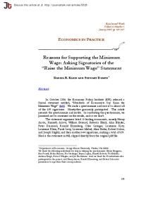
Figure 4 Hourly wage distribution for new hires from unemployment, LFS data

Actual hiring wages

6 hrwage

8

10

.2 .1 .05 0 2

4

6 hrwage

8

10

Fraction

8

10

2

4

6 hrwage

8

10

8

10

2010

0

0

.05

.1

.15

Fraction

.1 .2 .3

.2

2009

2

4

6 hrwage

8

10

8

10

8

10

0

0

.05

.1

.15

Fraction 6 hrwage

6 hrwage

2008

.2

.05 .15 .25 .1 .2

4

4

2007

0 2

2

.05 .15 .25 .1 .2

4

2006 Fraction

.15

Fraction

0

.05

.1

.15

Fraction

.15 .1 .05 0

Fraction

2

Fraction

2005

.2

2004

.2

2003

2

4

6 hrwage

31

2

4

6 hrwage

9

Tables

Table 1: NMW increases compared to growth in average weekly earnings (AWE) Adult rate

Date Apr 99 Oct00 Oct 01 Oct 02 Oct 03 Oct 04 Oct 05 Oct 06 Oct 07 Oct 08 Oct 09 Oct 10

AWE growth (%)

4.97 2.96 4.02 4.70 3.96 4.06 4.63 3.50 -0.23 2.03

NMW hourly rate £3.60 £3.70 £4.10 £4.20 £4.50 £4.85 £5.05 £5.35 £5.52 £5.73 £5.80 £5.93

NMW increase (%)

NMW increase minus AWE growth (%)

2.78 10.81 2.44 7.14 7.78 4.12 5.94 3.18 3.80 1.22 2.24

5.84 -0.52 3.12 3.08 0.17 1.88 -1.46 0.31 1.45 0.21

Youth development rate NMW NMW NMW increase hourly increase minus AWE rate (%) growth (%) £3.00 £3.20 6.67 £3.50 9.37 4.41 £3.60 2.86 -0.10 £3.80 5.56 1.53 £4.10 7.89 3.20 £4.25 3.66 -0.30 £4.45 4.71 0.64 £4.60 3.37 -1.26 £4.77 3.70 0.20 £4.83 1.26 1.48 £4.92 1.86 -0.17

Source: NMW rates from LPC (2010). AWE from ONS series KAB9, annual changes calculated to October each year.

Table 2 Sample sizes of new hires 2003

Males 69

Females 67

Total 136

2004

263

311

574

2005

241

292

533

2006

252

335

587

2007

305

394

699

2008

294

388

682

2009

277

319

596

2010

366

325

691

32

33

Table 3 Sample sizes for the horizontal DID, LFS data. Male adults Treated

Female adults

Control

Treated

18-21 year olds

Control

Treated

Control

Before

After

Before

After

Before

After

Before

After

Before

After

Before

After

2003

15

37

58

108

80

154

228

408

4

8

13

28

2004

159

113

176

174

513

413

470

487

22

17

90

74

2005

101

68

145

151

262

234

413

488

9

8

24

28

2006

84

79

138

138

300

282

363

395

3

3

26

24

2007

68

67

177

167

187

169

459

460

7

14

46

38

2008

129

90

189

199

348

359

461

477

7

5

30

21

2009

38

45

156

144

114

95

452

449

6

13

27

28

2010

35

21

175

91

113

70

476

240

7

6

27

10

34

35

Table 4 Sample sizes of additional control groups for the vertical DID for the employed, LFS data. Males Method 1 Control 2

Method 2

Control 3

Control 2

Method 3

Control 3

Control 2

Control 3

Before

After

Before

After

Before

After

Before

After

Before

After

Before

After

2003

91

199

77

187

58

108

58

108

6

198

162

36

2004

164

164

180

190

176

174

176

174

62

52

244

224

2005

170

168

127

157

145

151

145

151

100

72

170

186

2006

163

172

114

124

138

138

138

138

24

34

262

254

2007

136

154

143

140

177

167

177

167

228

282

62

2008

157

123

157

145

189

199

189

199

68

36

204

188

2009

120

130

153

167

156

144

156

144

150

146

2010

121

62

123

77

175

91

175

91

94

60

6

Females Method 1 Control 2

Method 2

Control 3

Control 2

Method 3

Control 3

Before

After

Before

After

Before

After

Before

After

2003

257

554

128

328

228

408

228

408

2004

367

368

323

326

470

487

470

487

2005

373

376

209

278

413

488

413

2006

334

332

208

227

363

395

2007

320

334

186

202

459

2008

241

269

221

219

2009

280

302

243

2010

270

121

197

Control 2 After

Before

After

540

458

94

208

98

450

570

488

84

182

208

126

363

395

34

78

504

466

460

459

460

176

124

242

372

461

477

461

477

94

112

298

320

267

452

449

452

449

350

330

78

476

240

476

240

264

130

36

Before

Control 3

50

Table 5 Sample sizes for the vertical DID exercise for the unemployed. Males Method 1

Method 2

Treated

Control 1

Control 2

Control 3

Treated

Control 1

Control 2

Control 3

2003

83

210

243

281

83

210

213

213

2004

122

206

229

271

122

206

242

258

2005

182

413

434

404

182

413

422

429

2006

176

410

400

433

176

410

506

563

2007

152

305

298

267

152

305

328

315

2008

265

506

501

481

265

506

515

517

2009

291

555

473

474

291

555

552

552

2010

289

563

501

468

289

563

614

618

Females Method 1

Method 2

Treated

Control 1

Control 2

Control 3

Treated

Control 1

Control 2

Control 3

2003

65

157

181

193

65

157

154

154

2004

118

216

205

194

118

216

180

164

2005

139

342

369

328

139

342

333

326

2006

218

448

328

295

218

448

352

295

2007

111

213

153

142

111

213

190

203

2008

205

408

444

359

205

408

399

397

2009

223

364

379

337

223

364

367

367

2010

193

414

376

295

193

414

363

359

37

Table 6 - Effects of NMW upratings on job retention for adult males. Horizontal DID estimates from linear probability models (1) (2) (3) (4) (5) (6) (7) (8) Treatment Dummy Treatment Dummy * Wage Gap 2003

-0.010 (0.091)

-0.020 (0.096)

-0.038 (0.086)

-0.040 (0.091)

-0.022 (0.083)

-0.032 (0.086)

-0.042 (0.079)

-0.044 (0.082)

2004

0.000 (0.050)

-0.038 (0.053)

0.020 (0.043)

-0.005 (0.045)

0.022 (0.047)

-0.000 (0.050)

0.037 (0.042)

0.021 (0.044)

2005

0.006 (0.062)

0.018 (0.067)

0.002 (0.057)

0.027 (0.061)

-0.022 (0.050)

-0.015 (0.052)

-0.022 (0.048)

-0.003 (0.050)

2006

0.129** (0.053)

0.112** (0.053)

0.123** (0.049)

0.116** (0.048)

0.051 (0.051)

0.043 (0.051)

0.063 (0.047)

0.061 (0.047)

2007

0.052 (0.059)

0.045 (0.060)

-0.028 (0.053)

-0.033 (0.054)

0.065* (0.038)

0.068* (0.040)

0.026 (0.036)

0.031 (0.037)

2008

0.067 (0.058)

0.098* (0.058)

-0.018 (0.050)

0.006 (0.049)

0.032 (0.051)

0.068 (0.050)

-0.025 (0.046)

0.007 (0.045)

2009

-0.033 (0.085)

-0.029 (0.090)

-0.079 (0.083)

-0.079 (0.088)

-0.032 (0.067)

-0.027 (0.070)

-0.058 (0.065)

-0.054 (0.069)

2010

-0.065 (0.111)

-0.115 (0.114)

-0.066 (0.106)

-0.084 (0.111)

-0.047 (0.107)

-0.107 (0.110)

-0.048 (0.103)

-0.086 (0.107)

29753 28754 29753 N no no yes Spill-over group no yes no Additional controls Coefficients from a linear probability model. Robust Standard errors in parentheses * p