The Effect of Density and Trip-Chaining on the Interaction between Urban Form and Transit Demand Sisinnio Concas and Joseph S. DeSalvo University of South Florida
Abstract It is unclear whether policies designed to reduce auto and increase transit usage achieve their objective. Evidence is mixed because most empirical research on these policies use ad hoc specifications, whereas our models are drawn from economic theory. Three models of increasing generality show how endogenizing relevant variables changes results obtained by others. The theoretical hypotheses are empirically tested using a dataset that integrates travel and land use. Our main findings are (1) population density has a small impact on transit demand, which decreases when residential location is endogenous; (2) households living farther from work use less transit, a result of trip-chaining; and (3) reducing the spatial allocation of non-work activities, improving transit accessibility at and around subcenters, and increasing the presence of retail locations in proximity to transit-oriented households would increase transit demand.
Introduction Recently, urban policies have sought to reduce presumed inefficiencies associated with urban sprawl. Since it is assumed the auto is the main cause of urban sprawl (Glaeser and Khan 2004), the policies are intended to produce a more compact urban area, which, presumably, would reduce auto usage and increase transit usage. Evidence favorable to such policies is mixed. The difficulty of generalizing findings is highlighted by the growing literature reviews and meta-analyses. In their most recent effort, Ewing and Cervero (2010) report that there are more than 200 studies in this topic, with two dozen surveys of the literature and two reviews of the many reviews. Most of this research involves regression of various measures of travel behavior on residential and employment density while controlling for traveler demographic characteristics. These studies have led to the conclusion that policy interventions to increase density are capable of reducing automobile use (Burchell et al. 1998; Cao et al. 2006; Ewing 1997). Nevertheless, criticism has centered on ad hoc specifications and omitted-variable bias. The former is due to lack of a theoretical foundation for the
Journal of Public Transportation, Vol. 17, No. 3, 2014 16
The Effect of Density and Trip-Chaining on the Interaction between Urban Form and Transit Demand
empirical work, and the latter is due to likely simultaneity and endogeneity in the relationship between urban form and travel (Badoe and Miller 2000). The influence of urban form on travel behavior is complicated by the evolution of the built environment, which might lead to residential self-sorting. “Self-sorting” refers to factors that induce households to choose a residential location, in part, due to idiosyncratic preferences for travel and location. If residential self-sorting is not accounted for, empirical findings overstate the efficacy of policies to affect travel behavior by changing the built environment. Mokhtarian and Cao (2008) provide a comprehensive review of empirical work on residential self-sorting. Although researchers recognize that idiosyncratic preferences for travel and location affect residential location, there is disagreement on how best to handle such preferences, which, if ignored, result in omitted-variable bias. The empirical treatment of omitted-variable bias in this context ranges from nested logit models (Cervero 2007) to sophisticated error-correlation models (Bowes and Ihlanfeldt 2001; Pinjari et al. 2007) and two-part models (Vance and Hedel 2007). Findings suggest that, after accounting for self-sorting, the built environment affects commute modechoice behavior. In addition, empirical work is lacking on the relationship between urban form and travel behavior that accounts for trip-chaining. A trip chain is defined as a sequence of trips linked together between two anchor destinations, such as home and work. The dearth of research on the effects of trip-chaining on the built environment is recognized by Ewing and Cervero (2009), who are unable to report land-use elasticity estimates in response to changes in multipurpose trip-chaining behavior. To our knowledge, there is no empirical work accounting for the joint determination of residential location, trip-chaining, the area of non-work activities, and socio-demographic differences among individuals, with a theoretical foundation based on the tradeoff between commuting and non-work travel. This paper attempts to fill this gap in the literature. We formulate three models of increasing generality. The purpose is to show how endogenizing relevant variables changes the results obtained by others. The theoretical hypotheses are empirically tested using a dataset that integrates travel and land-use.
Theory Introduction Economic analysis of the interaction between residential and work locations began with Alonso (1964), with important subsequent contributions by Mills (1972) and Muth (1969). In a budget-constrained, utility-maximization framework, the theory determines residential location as the result of a tradeoff between housing and transportation expenditures, given tastes, income, housing price, and transportation costs, in which all transportation for work and non-work activities is to the central business district (CBD) of the urban area. Individuals locate at a distance at which the marginal cost of transportation equals the marginal housing cost savings obtained by a move farther from the CBD. We retain this tradeoff but assume it occurs in a polycentric urban area, rather than a monocentric one. In this, we follow Anas and Kim (1996) and Anas and Xu (1999).
Journal of Public Transportation, Vol. 17, No. 3, 2014 17
The Effect of Density and Trip-Chaining on the Interaction between Urban Form and Transit Demand
Trip-chaining describes how travelers link trips between locations within an activity space. A trip from home to work with an intermediate stop to drop children off at day care is an example of a trip chain. Trip-chaining occurring on the home-job commute pair saves time. This time-saving, in turn, can be allocated either to additional non-work travel, thus increasing the overall demand for travel, or to a longer commute.1 The positive relationship between more complex trip chains and the home-work commute is confirmed by empirical work (Bhat 1997; Bhat 2001; Davidson 1991; Kondo and Kitamura 1987; McGuckin and Murakami 1999; Strathman 1995). Both residential location and trip-chaining take place within a geographical area called the activity space. Drawing on Anas (2007), we assume that the activity space results from utility-maximizing behavior determining non-work travel. Individuals prefer to visit different locations, a behavior that positively affects the size of the activity space. The activity space, therefore, accounts for the effect of the built environment on the spatial dispersion of out-of-home activities. The activity space follows from the time geographic concept of the space-time prisms first introduced by Hägerstrand (1970) and subsequently used to simulate travel behavior responses to space-time constraints (Timmermans et al. 2002). These variables all relate to travel demand, which we define as the number of work and non-work transit trips made by all members of a household. Finally, land use (which we proxy with population density) directly affects the spatial allocation of activities. The General Model These variables are brought together in the following general model (theoretically endogenous variables are in upper-case letters, while exogenous variables are in lower case).
TC = TC ( AS, RL,walk _ dist,veh,act _ tt,act _ dur, sch, subc _ dist ) AS = AS (TC, D,act _ dur,inc,r _ est )
TD = TD (TC, AS, RL,walk _ dist,tswork, prkride,ts _ tod,veh )
D = D ( RL, AS, subc _ dist,cbd _ dist )
(1) (2)
RL = RL (TC,TD,hprice,hage,rooms,div, pov,own )
(3) (4) (5)
Equation (1) describes trip-chaining behavior occurring on the commute trip. Trip chaining, jointly determined with the activity space (AS) and residential location (RL), is affected by transit station proximity (walk_dist), vehicle availability (veh), travel behavior (act_tt and act_dur), number of school-age children (sch), and the distance between home and the nearest subcenter (subc_dist). Equation (2) describes how the spatial extent of non-work activities (AS) responds to changes in urban form, being jointly determined with trip-chaining (TC) and urban form
1
Leisure time is another possibility, but that variable is not included in Anas (2007).
Journal of Public Transportation, Vol. 17, No. 3, 2014 18
The Effect of Density and Trip-Chaining on the Interaction between Urban Form and Transit Demand
(D). The activity space responds to the duration of non-work activities (act_dur), household income (inc), and retail establishment concentrations (r_est). Equation (3) describes the demand for transit trips (TD), due to non-work travel, which is jointly determined with trip-chaining (TC), the activity space (AS), and residential location (RL). Transit-station proximity (walk_dist) and the presence of a nearby transit stop (tswork) and of a park-and-ride facility (prkride) at the workplace also determine transit demand. To test the efficacy of transit-oriented-development policies in affecting ridership, we include the presence of a transit-oriented development near the residential unit (ts_tod). Finally, the number of autos at the disposal of the household (veh) also determines transit demand. Equation (4) describes residential location (RL), jointly determined with trip-chaining (TC) and transit demand (TD). We consider housing characteristics—pricing (hprice), age (hage), size (rooms), and tenure choice (own)—as factors affecting residential location, in addition to neighborhood characteristics, diversity (div) and poverty (pov). Equation (5) describes population density (D), as jointly determined with residential location (RL) and the activity space (AS). In addition, the equation introduces variables serving as proxies for centrality dependence (cbd_dist) and for polycentricity (subc_dist). Discussion of Our Choice of Variables Residential Location (RL) We define residential location as the job-residence pair (RL), measured as the distance in miles between home and work. This definition of residential location differs from that used in the current literature. Some researchers have considered residential location as a choice to reside within a geographical unit, such as a traffic assignment zone (Bhat and Guo 2004; Pinjari et al. 2007). Others have used transit proximity as a proxy for residential location (Cervero 2007). Although these usages are dictated by the need to distinguish the influence of the built environment from that of self-sorting, they are not based on a formal theory of residential location. For the variables affecting RL, we use household income (inc), median house price (hprice), and, as proxies for transportation cost, distance between home and the CBD (cbd_dist) and distance between home and the nearest subcenter (subc_dist). The use of distance measures as controls in multivariate analysis of transit travel behavior is a common practice (Cervero and Wu 1998; Kuby et al. 2004; Pushkarev and Zupan, 1977; Pushkarev and Zupan, 1982; Zupan and Cervero, 1996). We assume the location decision is based in part on idiosyncratic preferences for location and travel, which relaxes the assumption of common tastes in earlier models. To capture idiosyncratic preferences, we use house age (hage), number of rooms (rooms), and tenure choice, that is, whether the household is a renter or and owner (own). These variables control for housing preferences not directly affecting travel behavior but directly affecting the residential choice decision. To control for neighborhood characteristics, we include the percentage of households living below the poverty line (pov) and a diversity index (div). The former serves as a proxy for crime, while the latter is an index of ethnic heterogeneity that varies from 0 (only one race in the neighborhood) to 1 (no race is prevalent),
Journal of Public Transportation, Vol. 17, No. 3, 2014 19
The Effect of Density and Trip-Chaining on the Interaction between Urban Form and Transit Demand
similar to Shannon’s diversity index. The Shannon Index compares diversity between habitat samples in terms of the proportion of individuals of a given species in the set (see Begon, Harper, and Towsend [1996] for a review). Of these variables, house age has been used before as an instrumental variable in multivariate regression studies that considered travel behavior as endogenous to urban form (Boarnet and Crane 2001; Boarnet and Sarmiento 1998; Crane 2000; Crane and Crepeau 1998a; Crane and Crepeau 1998b), while the remaining ones are unique to this study although controls for neighborhood characteristics have been used elsewhere. For example, the proportion of block-group or census-tract population that is Black and the proportion Hispanic have been used as instruments by Boarnet and Sarmiento (1998) and the percent of foreigners by Vance and Hedel (2007). Trip Chaining (TC) In addition to determining residential location in a polycentric urban area, Anas’ theory (2007) also determines the sequence of non-work trip chains. To capture non-work trip chains, we use variables to control for factors affecting both the spatial extent of nonwork activities and the ensuing travel behavior, specifically, travel time (act_tt) and the duration of non-work activity (act_dur). To capture variables affecting trip-chaining, we use the number of school-age children (sch), the number of vehicles owned by the household (veh), and the number of retail establishments (r_est) in the activity space. These variables are commonly used in the activity-based literature in modeling activity duration and scheduling (Bhat 1997; Bhat 1999; Bhat 2001; Bhat and Guo 2004) and activity travel patterns (Kuppam and Pendyala 2001). Activity Space (AS) There are several ways to measure the activity space. The simplest measure is represented by the standard distance deviation (SDD), calculated as a standardized distance of outof-home activities from a mean geographic center. The mean activity center is analogous to the sample mean of a dataset, and it represents the sample mean of the x and y coordinates of non-work activities contained in each household activity set. Interpretation is relatively straightforward: a larger SDD indicates greater spatial dispersion of activity locations. Ebdon (1977) notes, however, that this measure is adversely affected by the presence of outliers. As a result of the squaring all the distances from the mean center, the extreme points have a disproportionate influence on the value of the standard distance. To attenuate this problem, we have chosen the standard distance ellipse (SDE), using the formula described in Levine (2005). These measures are illustrated in Figure 1.
Journal of Public Transportation, Vol. 17, No. 3, 2014 20
The Effect of Density and Trip-Chaining on the Interaction between Urban Form and Transit Demand
FIGURE 1. Standard distance circle and standard distance ellipse
The literature provides additional activity-space measures. For example, while Buliung and Kanaroglou (2006) use SDE, they also introduce the household activity space (HAS). HAS is an area-based geometry that defines a minimum convex polygon containing activity locations visited by a household during a reference period (i.e., the travel-survey period). The advantage of HAS is that it weights the activity space by the relevance of activities, such as their type (recreational, maintenance, etc.) and their relative frequencies. Although HAS reports an accurate geographical measurement of the activity space, Buliung and Remmel (2008) show that the use of the minimum convex polygon algorithm provides similar results to SDE in terms of behavioral interpretation. Other research shows that the choice of an appropriate shape representing an individual’s activity space is highly dependent on the spatial distributions and frequencies of the locations visited by the person in the given time period (Rai et al. 2007). We hypothesize that densely-populated urban areas exhibit clustered activity locations, thus shrinking the size of the activity space, while the opposite is the case for less densely-populated areas. This affects the spatial allocation of activities, which affects the demand for travel. Recent research finds that households residing in decentralized, lower-density urban areas have a more dispersed travel pattern than their counterparts residing in centralized, high-density urban areas (Buliung and Kanaroglou 2006; Maoh and Kanaroglou 2007). Travel Demand (TD) We define travel demand (TD) as the number of work and non-work transit trips at the household level, a usage that departs from that of other researchers. For example, Boarnet and Crane (2001) assume that trip demand is either directly affected by land use or indirectly by influencing the cost of travel. In our models, land use (which we proxy with population density, D) directly affects the spatial allocation of activities. Our measure of transit-station proximity (walk_dist) differs from that used elsewhere. Proximity is usually measured as the radius of a circular buffer around a station. Cervero
Journal of Public Transportation, Vol. 17, No. 3, 2014 21
The Effect of Density and Trip-Chaining on the Interaction between Urban Form and Transit Demand
(2007), for example, used a half-mile radius. This measure of transit proximity fails to account for barriers that prevent access to a station located within the radius, which is why we use walking distance from the residence to the nearest transit station. Empirical studies on the relevance of transit station proximity to transit patronage show a strong relationship between transit use and station proximity (Cervero 2007; Cervero and Wu 1998). We also include the following measures of transit supply to account for the presence of a transit stop near the workplace (tswork), the supply of park-and-ride facilities near a transit stop (prkride), and the presence of a transit-oriented development (ts_tod) near the residential unit. Population Density (D) In the long run, the simultaneous choice of location and travel decisions is assumed to affect density levels across a given urban area. Population density is treated as endogenous to the process and is affected by household travel decisions and location behavior. Aspects of this relationship and its influences on transit patronage have been previously considered in the literature. For example, while modeling long-run transit demand responses to fare changes, Voith (1997) treats density as endogenous and being affected directly by transit patronage levels. In the long run, these levels are affected by supply-side changes. Voith (1997) assumes that as transit services improve, more people tend to live in proximity to transit stations, thus increasing the demand for transit services. Empirically, we measure density, D, as gross population density of the Census block group in which the household residential unit is located. The Census block-group area is measured in square miles.
Data We use travel-diary data from the 2000 Bay Area Travel Survey (BATS2000). BATS2000 is a large-scale regional household travel survey conducted in the nine-county San Francisco Bay Area of California by the Metropolitan Transportation Commission (2008). Completed in the spring of 2001, BATS2000 provides consistent and rich information on travel behavior of 15,064 households with 2,504 households that make regular use of transit.2 Household activity locations are those visited by surveyed household members during a specified period—in this case, two representative weekdays. BATS2000 reports the longitude and latitude of each activity. Using geographic information systems (GIS), we geocoded to the street address or street intersection 99.9 percent of home addresses and 80 percent of out-of-home activities, giving us precise locations of non-work activities, jobs, and residences. Using GIS spatial matching procedures, we combined BATS2000 travel data with geographical data from the U.S. Census Bureau Summary File 3 and U.S. Census Bureau County Business Patterns (CBP), which gave us detailed social, economic, and housing characteristics at the block group level and variables related to non-residential land use, such as commercial densities. Table 1 contains the variable names, brief descriptions, and descriptive statistics. In MTC usage, a transit household has one or more members using transit at least once during the two-day surveying period. 2
Journal of Public Transportation, Vol. 17, No. 3, 2014 22
The Effect of Density and Trip-Chaining on the Interaction between Urban Form and Transit Demand
TABLE 1.
Variable
Variables and Descriptive Statistics
Description
Mean
inc
Household Income (1 if < $10k to15 if > $150k)
sch
S.D.
Min.
Max.
10.34
3.45
1.00
15.00
Number of children pre-k to middle school
0.65
0.98
0.00
7.00
veh
Household vehicles, number
1.85
0.95
0.00
9.00
own
Housing tenure (1=own, 0=renter)
0.69
0.46
0.00
1.00
walk_dist
Walking distance to nearest transit station, miles
0.31
0.37
0.00
3.00
tswork
Transit stop near work (1 within 0.5 mile, 0 otherwise)
0.25
0.43
0.00
1.00
prkride
Park & ride lot near work (1 within 0.5 mi., 0 otherwise)
0.07
0.25
0.00
1.00
ts_tod
TOD stop near residence (1 within 0.5 mi., 0 otherwise)
0.01
0.12
0.00
1.00
cbd_dist
Residential unit distance to CBD, miles
44.70
25.20
0.17
137.12
subc_dist
Residential unit distance to nearest subcenter, miles
2.89
2.36
0.01
38.39
r_est
Retail establishment density (number/mile2); ZIP code level
22.51
55.91
0.00
1,281.74
hprice
Median housing price, $; block group level
399,591
204,767
0
1,000,001
hage
Median housing age, year; block group level
35.49
14.86
1.00
61.00
rooms
Median number of rooms; block group level
5.92
1.04
0.00
9.10
pov
Proportion of households living below poverty level; block group level
0.06
0.06
0.00
0.79
div
Diversity index, 0=homogenous, 1= heterogeneous; block group level
0.58
0.19
0.00
0.99
act_dur
Non-work activity duration, minutes
act_tt
Travel time to non-work activity, minutes
TC
Stops on home-work route, number
TD
Household linked transit trips, number
AS RL D
Gross population density, persons/mile ; block group level
131.05
89.86
2.00
1,440
81.16
98.23
0.00
2,897
1.17
1.33
0.00
8.00
0.39
0.99
0.00
9.00
Household activity space, size of SDE; miles
16.83
32.61
0.75
437.23
Distance home-work, miles
10.52
9.81
0.00
79.38
9,144
11,065
0.00
172,400
2
2
Note: Means represent proportions for 0/1 variables.
Estimation Versions of the Model for Estimation Equations (1)–(3) of the general model constitute Model I, which treats residential location and density as exogenous. Given these variables, the model jointly defines the activity space and the trip chain, which, in turn, determine travel demand, given consumption and location decisions. This may be interpreted as a short-run model in that residential location and density are predetermined. Model II comprises Equations (1)–(4). In this extension, we relax the assumption of exogenous residential location. Treated as a choice variable, residential location is the outcome of a tradeoff between transportation and housing costs. Accounting for idiosyncratic
Journal of Public Transportation, Vol. 17, No. 3, 2014 23
The Effect of Density and Trip-Chaining on the Interaction between Urban Form and Transit Demand
preferences for transportation and location, households choose an optimal home-work commute, while optimizing non-work trip chaining and the activity space, which, in turn, determine transit demand. This may be interpreted as an intermediate-run model in that residential location is endogenous while density is exogenous. Model III is composed of Equations (1)–(5). In Equation (5) population density is endogenous. Explanatory variables serve as proxies for centrality dependence (cbd_dist) and for polycentricity (subc_dist).3 This may be interpreted as a long-run model in that it treats density (urban form) as endogenous. In the structural equations of the models, endogenous variables appear on the right-hand side. Consequently, estimation requires structural equation modeling (SEM), also called simultaneous equation modeling. SEM is used to capture the causal influences of the exogenous variables on the endogenous variables and the causal influences of the endogenous variables on one another. In the transportation literature there exist several applications of SEM using cross-sectional data, for example, Pendyala (1998), Fuji and Kitamura (2000), and Golob (2000). Additional examples are discussed by Golob (2003). There are also studies of the causal relationships among travel behavior and urban form that are effectively represented in a structural equation framework (Cao et al. 2007; Guevara and Moshe 2006; Mokhtarian and Cao 2008; Peng et al. 1997). Model I: Endogenous Trip-Chaining, Activity Space, and Transit Demand In this specification, residential location (RL) and density (D) are exogenous. Given these variables, the model jointly determines the trip chain (TC), the activity space (AS), and transit demand (TD).
The equations of Model I are estimated by three-stage least squares (3SLS). All three equations pass the rank condition for identification. The first equation is overidentified, and the other two are just identified.4 The results are given in Table 2. To ensure normality assumptions are met, some of the variables are entered in logs, namely, AS, D, and walk_ dist.
3
Endogeneity tests led to cbd_dist, subc_dist, and r_est being treated as endogenous in Model III.
4
Details are in an unpublished appendix available on request.
Journal of Public Transportation, Vol. 17, No. 3, 2014 24
The Effect of Density and Trip-Chaining on the Interaction between Urban Form and Transit Demand
The joint determination of trip chaining and the spatial extent of non-work activities relate to transit patronage as hypothesized earlier. The presence of a transit stop at the workplace (tswork) positively affects transit demand, as does the presence of a TOD transit stop in proximity to the residence (ts_tod). The size of the activity space reduces as density increases, which, in turn, positively affects the demand for transit. At locations where non-work activities are more clustered, the need to engage in journeys requiring modes other than transit decreases, resulting in increased transit usage. This finding suggests that policies affecting the clustering of non-work activities, such as mixed land-use policies, are likely to significantly affect transit ridership levels. The relevance of this relationship is better appreciated, however, when residential location is endogenous. TABLE 2. Regression Results for Model I
Equation
Coefficient
p-value
(1) Trip chaining, TC 0.0648
AS
0.6960
0.0096
0.0160
walk_dist
–0.0570
0.0000
veh
–0.0793
0.0100
0.0014
0.0010
RL
act_tt
–0.0022
0.0000
subc_dist
0.0439
0.0000
sch
0.0778
0.0000
constant
1.2771
0.0000
TC
0.5863
0.0000
D
–0.0974
0.0000
0.0001
0.6880
act_dur
(2) Activity space, AS
act_dur
0.0299
0.0000
–0.0022
0.0000
1.7226
0.0000
TC
–0.6548
0.0000
AS
–0.3002
0.0010
RL
–0.0057
0.0070
walk_dist
–0.0800
0.0000
tswork
0.3848
0.0000
prkride
–0.0737
0.1510
ts_tod
0.2063
0.0600
–0.0456
0.0390
–0.1256
0.2150
inc r_est constant (3) Transit demand, TD
veh constant N= 8,229; χ
2 TC
=589.8; χ
2 AS
=514.4; χ =1,697.5 2 TD
Journal of Public Transportation, Vol. 17, No. 3, 2014 25
The Effect of Density and Trip-Chaining on the Interaction between Urban Form and Transit Demand
To appreciate the magnitude of the estimated effects, Table 3 reports point elasticities of transit demand with respect to selected explanatory variables. Elasticities are evaluated at data means and, because the models involve at least three simultaneous equations, are complicated to calculate.5 TABLE 3. Selected Elasticities for Model I
Elasticity
RL
TC
0.090
AS TD
D
walk_dist
subc_dist
r_est
tswork*
ts_tod*
–0.006
–0.051
0.113
–0.047
-
-
0.062
–0.101
–0.035
0.077
–0.051
-
-
–0.097
0.089
–0.079
–0.282
0.045
0.385
0.206
*Indicates a proportional change.
Table 3 shows that a 20-percent increase in gross population density (D), equal to about 1,830 persons per square mile, produces a 1.8-percent increase in transit demand (TD). A doubling of the average walking distance (walk_dist) to the nearest transit station, an increase from 0.3 miles to 0.6 miles, decreases transit demand by 7.9 percent; at about 1 mile, transit demand declines by 18.5 percent. The presence of a transit station within a half-mile of the workplace (tswork) increases transit demand by 38.5 percent. Living in proximity to a TOD transit station (ts_tod) increases transit demand by about 20.6 percent. There is a ridership bonus for proximity to a station with accessibility features to promote transit use. We find a negative elasticity between residential location (RL) and transit use. This is consistent with the hypothesis that households with longer commutes engage in more complex trip chains, which positively affect the spatial extent of non-work activities. With exogenously fixed transit supply, as the activity space expands, transit demand declines. The results also show that transit demand is sensitive to the presence of nearby subcenters (subc_dist) or, in general, to decentralization. The farther a household lives from a subcenter, the less it uses transit. A 50 percent increase in distance to a subcenter, from 2.9 to 4.3 miles, decreases transit demand by about 14.1 percent. This happens because households rely more on other modes to carry out complex trip chains, a finding confirmed by the elasticity of trip-chaining with respect to distance to the nearest subcenter. This result is consistent with the current literature on transit competitiveness and polycentric metropolitan regions. For example, Casello (2007) finds that transit improvements between and within subcenters are necessary to realize the greatest improvements in transit performance. Model II: Endogenous Trip-Chaining, Activity Space, Transit Demand, and Residential Location In this extension, we relax the assumption of exogenous residential location. Given density, the model jointly determines the trip chain, the activity space, transit demand, and residential location. The equations of Model II are estimated by three-stage least squares (3SLS). All four equations pass the rank condition for identification.
Two unpublished appendices are available at request that detail the comparative static analyses and the elasticity calculations. 5
Journal of Public Transportation, Vol. 17, No. 3, 2014 26
The Effect of Density and Trip-Chaining on the Interaction between Urban Form and Transit Demand
The first equation is overidentified, and the other three of just identified. The results are given in Table 4.
Journal of Public Transportation, Vol. 17, No. 3, 2014 27
The Effect of Density and Trip-Chaining on the Interaction between Urban Form and Transit Demand
TABLE 4.
Equation
Regression Results for Model II
Coefficient
p-value
(1) Trip chaining, TC AS
0.0725
0.7140
RL
0.0096
0.4130
walk_dist
–0.0573
0.0000
veh
–0.0786
0.0130
0.0014
0.0020
–0.0022
0.0000
subc_dist
0.0435
0.0000
sch
0.0778
0.0000
constant
1.2604
0.0000
act_tt act_dur
(2) Activity space, AS 0.2357
0.0000
D
–0.0858
0.0000
act_dur
–0.0007
0.0000
hhinc
0.0412
0.0000
r_est
–0.0014
0.0000
2.0943
0.0000
–0.6964
0.0000
AS
–0.2598
0.0250
RL
–0.0090
0.3110
walk_dist
–0.0669
0.0000
tswork
0.3716
0.0000
prkride
–0.0669
0.2020
ts_tod
0.1304
0.2560
veh
–0.0365
0.0990
constant
–0.1119
0.2720
TC
3.7324
0.0000
TD
–1.2408
0.0080
hprice
–2.8117
0.0000
hage
–0.0849
0.0000
1.1279
0.0000
div
–2.6312
0.0000
pov
–5.9629
0.0130
own
0.4966
0.0620
TC
constant (3) Transit demand, TD TC
(4) Residential location, RL
rooms
39.1808
constant N= 8,212; χ
2 TC
=341.5; χ
2 AS
0.0000
=419.9; χ =1845.0; χ = 444.8 2 TD
2 RL
Journal of Public Transportation, Vol. 17, No. 3, 2014 28
The Effect of Density and Trip-Chaining on the Interaction between Urban Form and Transit Demand
Table 5 reports selected point elasticities for statistically significant estimates. Compared to Model I, endogenous residential location reduces the magnitude of the elasticity of travel demand with respect to density by 19 percent. When households can locate anywhere in an urban area and when they adjust trip chaining and commuting costs, an exogenous 20-percent increase in density produces a 1.4-percent increase in the demand for transit. TABLE 5.
Elasticity
Selected Elasticities from Model II
D
walk_dist
subc_dist
r_est
tswork*
TC
–0.006
–0.052
0.115
–0.002
–
AS
–0.087
–0.014
0.032
–0.033
–
TD
0.072
–0.051
–0.277
0.028
0.372
RL
–0.006
–0.002
0.060
–0.002
–
*Indicates a proportional change.
Accounting for self-sorting, through choice of residential location, reduces the relevance of transit-station proximity to the residence, indicated by a 35-percent decrease in magnitude in the point elasticity estimate with respect to Model I. An increase from 0.3 to 0.6 miles to the nearest transit station reduces transit demand by only 5.1 percent, as opposed to the 7.9-percent reduction of Model I. This result shows that self-sorting is less relevant than Cervero (2007) noted. He found that self-sorting accounts for about 40 percent of transit ridership for individuals residing near a transit station. The specification of Model II helps us understand the reasons for the changes from Model I. In Model II, households optimally choose residential location and non-work activities, choices that optimally define the spatial extent of non-work activities. Households locate their residences farther from their job locations, trading lower housing costs for increased commute distance. Trip chaining optimization is part of this tradeoff, which leads to an expansion of the activity space. This, in turn, reduces opportunities to use transit for non-work travel. This behavior is empirically validated by the statistical significance of all housing and neighborhood controls in the residential location equation. Model III: Endogenous Trip-Chaining, Activity Space, Transit Demand, Residential Location, and Density In this extension, we relax the assumption of exogenous density at the residential unit location. The model jointly determines the trip chain, the activity space, transit demand, residential location, and density.
Journal of Public Transportation, Vol. 17, No. 3, 2014 29
The Effect of Density and Trip-Chaining on the Interaction between Urban Form and Transit Demand
All five equations pass the rank condition for identification. The first equation is overidentified, and the other equations are just identified. The equations of Model III are estimated by three-stage least squares (3SLS). The results are given in Table 6. In the long run, the simultaneous choice of location and travel affects urban density. Aspects of this relationship have been considered in the literature. For example, while modeling long-run transit demand responses to fare changes, Voith (1997) treats density as endogenous and as being affected directly by transit patronage levels. In the long run, these levels are affected by supply-side changes. Voith (1997) assumes that as transit services improve, more people live in proximity to transit stations, thus increasing the demand for transit services. Our estimation shows that both CBD and subcenter distance from the residence are statistically significant in determining density. The signs of cbd_dist and subc_dist are negative, as expected.
Journal of Public Transportation, Vol. 17, No. 3, 2014 30
The Effect of Density and Trip-Chaining on the Interaction between Urban Form and Transit Demand
TABLE 6.
Equation
Regression Results for Model III
Coefficient
p-value
AS
1.00867
0.0000
RL
0.07774
0.0000
walk_dist
–0.66261
0.0000
veh
–0.02917
0.3570
act_tt
–0.00093
0.0560
act_dur
–0.00036
0.2650
0.18745
0.0000
(1) Trip chaining, TC
subc_dist
0.05695
0.0000
–2.93691
0.0000
0.53891
0.0000
D
–0.28170
0.0000
act_dur
–0.00004
0.8390
hhinc
0.01819
0.0000
r_est
–0.00177
0.0790
3.51093
0.0000
TC
–0.23095
0.0030
AS
0.21302
0.0540
RL
0.01619
0.0700
sch constant (2) Activity space, AS TC
constant (3) Transit demand, TD
–0.47395
0.0000
tswork
0.44630
0.0000
prkride
–0.07878
0.0840
walk_dist
0.12797
0.1980
veh
–0.06411
0.0020
constant
–1.31138
0.0000
TC
2.46949
0.0000
TD
–1.16775
0.0130
hprice
–2.79304
0.0000
hage
–0.09605
0.0000
1.34316
0.0000
div
–6.19042
0.0000
pov
–4.50750
0.0060
ts_tod
(4) Residential location, RL
rooms
1.37799
0.0000
40.31047
0.0000
RL
–0.00907
0.4000
AS
–0.53331
0.0000
cbd_dist
–0.04010
0.0000
subc_dist
–0.07071
0.0190
own constant (5) Density, D
11.76875
constant
N= 8,212; χ
2 TC
=2,512.8; χ =611.2; χ 2 AS
2 TD
0.0000
=1,712.7; χ =646.3; χ2D=1,448.6 2 RL
Journal of Public Transportation, Vol. 17, No. 3, 2014 31
The Effect of Density and Trip-Chaining on the Interaction between Urban Form and Transit Demand
Findings Table 7 compares the point elasticities of Model III with preceding estimates and summarizes our main findings. We find that exogenous density change does not have a large effect on transit demand, and the magnitude of the effect decreases when residential location becomes endogenous. A 20-percent increase in gross population density (1,830 persons per square mile) increases transit demand from a minimum of 1.4 percent to a maximum of 1.8 percent. Treating density endogenously results in a more elastic travel demand with respect to distance to the nearest transit center. The elasticity of transit demand with respect to distance to the CBD (–0.09) is substantially less in absolute value than the elasticity with respect to distance to the nearest subcenter (–0.45). TABLE 7. Selected Transit-Demand Elasticities6
Elasticity Density
Model Ia
Model IIb
Model IIIc
0.089
0.072
na
–0.079
–0.051
–0.769
Transit station at workplace*
0.385
0.372
0.446
TOD station*
0.206
na
na
na
na
–0.087
Distance to nearest subcenter
–0.282
–0.277
–0.385
Retail establishments density
0.045
0.028
0.077
–0.097
na
na
Walking distance
Distance to CBD
Residential location
Residential location and density exogenous. b Density exogenous. c All endogenous. na = not available. *Indicates a proportional change. a
Subcenters play a more important role, and our findings support a policy of providing transit services in decentralized employment and residential areas to increase ridership. In other words, transit patronage is more responsive to a residential location near a subcenter than near the CBD. This result is consistent with recent findings of increased transit use in better served decentralized urban areas (Brown and Thompson 2008; Thompson and Brown 2006) and findings showing that transit ridership is not affected by the CBD (Brown and Nego 2007). The importance of station proximity to transit demand decreases after accounting for idiosyncratic preferences for location. In Model II, the elasticity of transit demand with respect to walking distance is about one-third smaller than in Model I, in which residential location and density are exogenous. This decline in magnitude results from allowing households to choose their residential location and by accounting for omitted-variable
The variables cbd_dist, subc_dist, and r_est appear as explanatory variables but are treated as endogenous in Model III. An initial specification treated these three variables as exogenous, but overidentification tests show that this treatment led to weak instruments, a problem leading to inconsistent estimates. McMillen (2001) finds that subcenters are endogenous to density. 6
Journal of Public Transportation, Vol. 17, No. 3, 2014 32
The Effect of Density and Trip-Chaining on the Interaction between Urban Form and Transit Demand
bias. On the other hand, the endogenous treatment of density and station proximity results in a much higher elasticity (–0.77). Transit station proximity to a workplace also has a significant positive impact on ridership, as indicated by the magnitude of the proportional changes across all three models. Likewise, in Model I transit-oriented development near transit stations has a positive impact on transit use; a TOD stop increases transit demand by about 21 percent. A transit station near a workplace exerts a positive impact on ridership, as indicated by the magnitude of the proportional changes across all three models. The importance of mixed-use development to increase transit patronage is highlighted by the elasticity of travel demand with respect to retail establishment density. Model II shows that a 20-percent increase in retail establishment density (or about 28 establishments per square mile) increases transit demand by 1.5 percent. Households living farther from work use less transit, which is due to trip-chaining behavior. Such households engage in complex trip chains and have, on average, a more dispersed activity space, which requires reliance on more flexible modes of transportation. The results support policies that would reduce the spatial allocation of activities and improve transit accessibility at and around subcenters. Similar results can be obtained by policies that increase the presence of retail locations in proximity to transit-oriented households.
Conclusions The debate on the relationship between urban form and transit travel has shifted from the need to determine minimum density thresholds that support transit to the need to provide reliable information to guide decision makers about what mix of land-use policies would better promote transit use. The models developed in this paper move towards this direction by studying the relationship between transit travel and the built environment in an increasingly suburban environment and decentralized employment. By explicitly acknowledging the complexity of travel arrangements (i.e., trip-chaining), we show that land-use policies can be successful in increasing transit patronage. The results of our work indicate that while population density is a factor in determining demand, targeting landuse policies affecting residential location decisions and development in suburban areas can be more effective. The models of this study require a substantial amount of information, not only in terms of travel behavior data from travel diaries, but also on the spatial location of residences, work, and non-work activities. The increased sophistication of communication systems that can easily track individuals’ travel patterns in space and time is making the data-collection effort less daunting, allowing increased used of sophisticated models, such as the ones developed in this paper. Notwithstanding the validity of the post-estimation tests, there still exists the possibility of endogeneity of some of the exogenous variables. This endogeneity, although confuted by statistical tests, is not ruled out by theoretical assumptions. For example,
Journal of Public Transportation, Vol. 17, No. 3, 2014 33
The Effect of Density and Trip-Chaining on the Interaction between Urban Form and Transit Demand
while this study treats vehicle ownership as exogenous and not directly influenced by the location decision, the literature contains studies that consider vehicle ownership as a discrete-choice variable endogenous to the residential location process and to density levels (Spissu et al. 2009). As discussed in this paper, the implications of treating a variable as exogenous, while being endogenous to the process, are not trivial. Finally, the behavioral models we presented rely on the assumption that households can save time by engaging in trip chaining. Time savings are then reallocated to either more non-work travel or to an extended commute. The model does not explicitly explain what happens to leisure time. The inclusion of total time constraints that include all relevant time uses (in-home and out-of-home) could provide additional insight on time use and its effect on trip chaining.
References Alonso, W. 1964. Location and Land Use. Harvard University Press, Cambridge. Anas, A. 2007. A unified theory of consumption, travel and trip chaining. Journal of Urban Economics 62: 162-186. Anas, A., and I. Kim. 1996. General equilibrium models of polycentric urban land use with endogenous congestion and job agglomeration. Journal of Urban Economics 40: 232256. Anas, A., and R. Xu. 1999. Congestion, land use and job dispersion: A general equilibrium analysis. Journal of Urban Economics 45(3): 451-473. Badoe, D. A., and E. J. Miller. 2000. Transportation–land-use interaction:Empirical findings in North America, and their implications for modeling. Transportation Research Part D 5: 235-263. Begon, M., J. L. Harper, and C. R. Townsend. 1996. Ecology: Individuals, Populations, and Communities, 3rd ed., Blackwell, Oxford. Bhat, C. 1997. An econometric framework for modeling the daily activity-travel pattern of individuals. Activity-Based Workshop, National Institute of Statistical Sciences, North Carolina Bhat, C. 1999. An analysis of evening commute stop-making behavior using repeated choice observations from a multi-day survey. Transportation Research Part B. Methodological 33(6): 495-510. Bhat, C. 2001. Modeling the commute activity-travel pattern of workers. formulation and empirical analysis. Transportation Science 35(1): 61-79. Bhat, C., and J. Guo. 2004. A mixed spatially correlated logit model. formulation and application to residential choice modeling. Transportation Research Part B. Methodological 38: 147-168. Boarnet, M. G., and R. Crane. 2001. Travel by design: The influence of urban form on travel. In Spatial Information Systems, Oxford University Press, Oxford, New York, 33-59.
Journal of Public Transportation, Vol. 17, No. 3, 2014 34
The Effect of Density and Trip-Chaining on the Interaction between Urban Form and Transit Demand
Boarnet, M. G., and S. Sarmiento. 1998. Can land-use policy really affect travel behaviour? A study of the link between non-work travel and land-use characteristics. Urban Studies 35(7): 1155-1169. Bowes, D. R., and K. R. Ihlanfeldt. 2001. Identifying the impacts of rail transit stations on residential property values. Journal of Urban Economics 50: 1-25. Brown, J. R., and D. Nego. 2007. Urban structure and transit ridership: A reexamination of the relationship in the United States. 87th Annual Meeting of the Transportation Research Board, Washington, DC. Brown, J. R., and G. L. Thompson. 2008. The relationship between transit ridership and urban decentralization. Insights from Atlanta. Urban Studies 45(5-6): 1119-1139. Buliung, R., and P. Kanaroglou. 2006. Urban form and household activity-travel behavior. Growth and Change 37: 174-201. Buliung, R., and T. K. Remmel. 2008. Open source, spatial analysis, and activity-travel behavior research. Capabilities of the Aspace package. Journal of Geography Systems 10: 191-216. Burchell, R. W., N. A. Shad, D. Listokin, and H. Phillips, H. 1998. The cost of sprawl – revisited. Transportation Research Board, Washington, DC. Cao, X., P. L. Mokhtarian, and S. I. Handy. 2006. Examining the impacts of residential self-selection on travel behavior: Methodologies and empirical findings. University of California. Cao, X., P. L. Mokhtarian, and S. I. Handy 2007. Do changes in neighborhood characteristics lead to changes in travel behavior? Structural equations modeling approach. Transportation, 35(5), 535-556. Casello, J. M. 2007. Transit competitiveness in polycentric metropolitan regions. Transportation Research Part A 41: 19-40. Cervero, R. 2007. Transit oriented development’s ridership bonus. a product of self selection and public policies. Environment and Planning A 39(9): 2068-2085. Cervero, R., and K.-L. Wu. 1998. Sub-centring and commuting: Evidence from the San Francisco Bay area, 1980-90. Urban Studies 35(7): 1059-1076. Crane, R. 2000. The influence of urban form on travel. an interpretive review. Journal of Planning Literature 15(1): 1-23. Crane, R., and R. Crepeau. 1998a. Does neighborhood design influence travel? A behavioral analysis of travel diary and GIS data, University of California Transportation Center, Berkeley. Crane, R., and R. Crepeau. 1998b. Does neighborhood design influence travel? A behavioral analysis of travel diary and GIS data. Transportation Research Part D 3(4): 225238. Davidson, D. 1991. Impact of suburban employee trip chaining on transportation demand management. Transportation Research Record 1321: 82-89.
Journal of Public Transportation, Vol. 17, No. 3, 2014 35
The Effect of Density and Trip-Chaining on the Interaction between Urban Form and Transit Demand
Ebdon, D. 1977. Statistics in Geography. A Practical Approach. Blackwell Publishing, Oxford. Ewing, R. 1997. Is Los Angeles-Style sprawl desirable? Journal of the American Planning Association 63: 107-126. Ewing, R., and R. Cervero. 2010. Travel and the built environment. Journal of the American Planning Association 76(3): 1-30. Fuji, S., and R. Kitamura. 2000. Evaluation of trip-reducing effects of new freeways using a structural equations model system of commuters’ time use and travel. Transportation Research Part B. Methodological 34: 339-354. Glaeser, E. L. and M. E. Khan. 2004. Sprawl and urban growth. In Handbook of Regional and Urban Economics, Vol. 4, ed. J. V. Henderson & J.-F. Thisse, Elsevier North Holland, Amsterdam. Golob, T. F. 2000. A simultaneous model of household activity participation and trip chain generation. Transportation Research Part B. Methodological 34(5): 355-376. Golob, T. F. 2003. Structural equation modeling for travel behavior research. Transportation Research Part B. Methodological 37(1): 1-25. Guevara, C. A., and B.-A. Moshe. 2006. Endogeneity in residential location models. Transportation Research Record, 1977. Hägerstrand, T. 1970. What about people in regional science? Papers of the Regional Science Association 24: 7-21. Kondo, K., and R. Kitamura. 1987. Time-space constraints and the formation of trip chains. Regional Science and Urban Economics 17: 49-65. Kuby, M., A. Barranda, and C. Upchurch. 2004. Factors influencing light-rail station boardings in the United States. Transportation Research Part A 38: 223-247. Kuppam, A. K., and R. M. Pendyala. 2001. A structural equation analysis of commuters’ activity and travel patterns. Transportation 28: 35-54. Levine, N. 2005. Crimestat III. A spatial statistics program for the analysis of crime incident locations. National Institute of Justice, Washington, DC. Maoh, H., and P. Kanaroglou. 2007. Geographic clustering of firms and urban form: A multivariate analysis. Journal of Geography Systems 9: 229-252. McGuckin, N., and E. Murakami. 1999. Examining trip-chaining behavior: Comparison of travel by men and women. Transportation Research Record 1693: 79-85. Metropolitan Transportation Commission. Household Travel Survey Data & Reports. Available from . Mills, E. S. 1972. Studies in the Structure of the Urban Economy. Johns Hopkins University Press, Baltimore.
Journal of Public Transportation, Vol. 17, No. 3, 2014 36
The Effect of Density and Trip-Chaining on the Interaction between Urban Form and Transit Demand
Mokhtarian, P. L., and X. Cao. 2008. Examining the impacts of residential self-selection on travel behavior: A focus on methodologies. Transportation Research Part B. Methodological 42: 204-228. Muth, R. F. 1969. Cities and Housing. The Spatial Pattern of Urban Residential Land Use. University of Chicago Press, Chicago. Pendyala, R. 1998. Causal analysis in travel behavior research: A cautionary note, in Travel Behaviour Research. Updating the State of Play, ed. S. Jara-Diaz, Pergamon, Oxford, 35-48. Peng, Z.-R., K. J. Duecker, J. Strathman, and J. Hopper. 1997. A simultaneous route-level transit patronage model. Transportation 24: 159-181. Pinjari, A. R., R. M. Pendyala, C. R. Bhat, and P. A. Waddel. 2007. Modeling residential sorting effects to understand the impact of the built environment on commute mode choice. Transportation 34: 557-573. Pushkarev, B., and J. M. Zupan. 1977. Public Transportation and Land Use Policy. Indiana University Press, Bloomington. Pushkarev, B. S., and J. M. Zupan. 1982. Urban Rail in America: An Exploration of Criteria for Fixed-Guideway Transit. Fitzhenry & Whiteside, Ontario, Canada. Rai, R. K., M. Balmer, M. Rieser, V. S. Vaze, S. Schonfelder, and K .W. Axhausen. 2007. Capturing human activity spaces. Transportation Research Record 2021: 70-80. Spissu, E., A. R. Pinjari, R. Pendyala, and C. Bhat. 2009. A Copula-based joint multinomial discrete-continuous model of vehicle type choice and miles of travel. Transportation 36(4): 403-422. Strathman, J. G. 1995. Understanding trip chaining—Special report on trip and vehicle attributes. U.S. Department of Transportation, Washington, DC. Thompson, G. L., and J. R. Brown. 2006. Explaining variation in transit ridership in U.S. metropolitan cities between 1990 and 2000. A multivariate analysis. Transportation Research Record 1986: 172-181. Timmermans, H., T. Arentze, and C.-H. Joh. 2002. Analysing space-time behaviour: New approaches to old problems. Progress in Human Geography 26(2): 175-190. Vance, C., and R. Hedel. 2007. The impact of urban form on automobile travel: Disentangling causation from correlation. Transportation 34: 575-588. Voith, R. 1997. Fares, service levels, and demographics: What determines commute rail ridership in the long run? Journal of Urban Economics 41: 176-197. Zupan, J., and R. Cervero. 1996. Commuter and Light Rail Transit Corridors. The Land Use Connection. Transportation Research Board, National Research Council.
Journal of Public Transportation, Vol. 17, No. 3, 2014 37
The Effect of Density and Trip-Chaining on the Interaction between Urban Form and Transit Demand
About the Authors Sisinnio Concas (
[email protected]) is a Research Associate Professor at the Center for Urban Transportation Research at the University of South Florida. His research interests are in urban economics, with a focus on the linkages between urban form, residential location, and travel patterns.
Joseph S. DeSalvo (
[email protected]) is a Professor in the Department of Economics at the University of South Florida. His teaching and research interests are in urban and regional economics, including especially location of households and firms, urban structure, housing economics, and transportation economics.
Journal of Public Transportation, Vol. 17, No. 3, 2014 38