EDHEC RISK AND ASSET MANAGEMENT RESEARCH CENTRE EDHEC — 393–400 promenade des Anglais, 06202 Nice — Tel. +33 (0)4 93 18 78 24 — Fax. +33 (0)04 93 18 78 40 Email: [email protected] — Web: www.edhec-risk.com

Structural Sources of Return and Risk in Commodity Futures Investments Hilary Till Principal, Premia Capital Management, LLC Research Associate with the EDHEC Risk and Asset Management Research Centre

April 2006

Author’s Note: This article originally appeared in the June 2006 edition of Commodities Now: http://www.commodities-now.com.

EDHEC is one of the top five business schools in France owing to the high quality of its academic staff (100 permanent lecturers from France and abroad) and its privileged relationship with professionals that the school has been developing since its establishment in 1906. EDHEC Business School has decided to draw on its extensive knowledge of the professional environment and has therefore concentrated its research on themes that satisfy the needs of professionals. EDHEC pursues an active research policy in the field of finance. Its Risk and Asset Management Research Centre carries out numerous research programs in the areas of asset allocation and risk management in both the traditional and alternative investment universes. Copyright © 2006 EDHEC

2

Performance and Asset Review By now it has become well-known that commodities have had superior performance over the past four and a half years. Figure 1 reviews just how superior that performance has been: from December 2001 through April 2006, the Goldman Sachs Commodity Index (GSCI) has returned 23.1% per year while the S&P 500 has returned a more modest 4.9% per year. Given these returns, commodity investing has become a sign of sophistication. Commodities can give “turbo returns if things go wrong for equities and bond markets,” stated the chief investment officer of a large British pension plan, as quoted in Rees (2006). The significant growth in commodity index investing is shown in Figure 2. New commitments from pension funds have fueled some of this growth. “Even normally cautious British pension funds are following the more adventurous US precedents and are allocating assets to commodities: the Sainsbury fund has targeted a 5% exposure, the British Telecom fund just under 3%. ... Global pension funds are estimated by investment consultants Watson Wyatt to be worth $16 trillion and if they, like the BT fund, were to allocated 3% to commodities, this would amount to $500bn cascading into what have been quite narrow markets,” noted a Financial News (2006) story. Because commodity index investing has grown from an obscure, niche strategy to a more widely accepted investment, there has been a need to better understand the drivers of historical commodity returns and risks. An investor would presumably then be in a better position to make informed judgments on the future prospects of a commodity investment. This article will provide the busy reader with a summary of the new research on this topic.

3

Historical Returns A recent edition of the prestigious Financial Analysts Journal (FAJ) included two articles, which explored the historical returns of commodity futures indices. Gorton of the University of Pennsylvania and Rouwenhorst of Yale University studied the properties of commodity futures over the period, 1959 though 2004, in the article, “Facts and Fantasies about Commodity Futures,” in the March/April 2006 FAJ. Gorton and Rouwenhorst created a monthly time series, starting in 1959, of an equallyweighted index of commodity futures. Their index was rebalanced monthly. They found that over the time period of their study that fully collateralized commodity futures historically had offered the same return and Sharpe ratio as U.S. equities. (The Sharpe ratio is calculated as an investment’s excess returns over Treasury bills, divided by the investment’s standard deviation.) Figure 3 summarizes the historical excess returns of their commodity futures index versus the returns of stocks and bonds. Stocks are represented by the S&P 500 index, and bonds are represented by the Ibbotson U.S. corporate bond index. Again, “excess returns” means that these are the returns over an investment in risk-less Treasury bills. They also found that commodity futures returns were negatively correlated with equity and bond returns. This means that over the time period of their study, a commodity futures investment would have added a new source of returns for an investor, not accessible through stock and bond investments. Decomposition of Historical Returns: Rebalancing, Term-Structure Characteristics, and Paradigm Shifts The Gorton and Rouwenhorst study is very valuable in providing investors with a carefully updated examination of historical commodity returns. An additional area of fertile research has been to understand what the drivers of those historical returns were. One highly nuanced point about commodity futures investing is that historically their long-term returns did not rely on broad-based rallies in spot commodity prices. For example, the second column in Figure 4 shows how the spot prices of a number of commodities ranged between -2.8% to +3.3% per year from 1983 to 2004. The first column in Figure 4 shows for each commodity, how much a commodity’s futures returns can be different from its spot returns. The source of these substantial differences will be explained below in the “Term-Structure Characteristics” section of this article. Another highly nuanced point is that when one combines individual commodity contracts into an index and then actively rebalances their weights periodically, that rebalancing can also be an additional source of return for a commodity investor. This effect is not obvious when only examining individual commodity futures contract returns since this is a portfolio-level effect. This effect, in turn, will be discussed below in the “Rebalancing” section of this article.

4

We will also discuss another source of returns, which has scant historical evidence, but nonetheless may have relevance for commodity investors going forward, and that is a rare trend shift in spot commodity prices, as occurred during 1970-to-1974. This scenario will be discussed below in the “Paradigm Shift: The 1970’s Revisited” section of this article. Rebalancing In a second March/April 2006 FAJ article, Erb of Trust Company of the West and Harvey of Duke University carefully dissect the historical drivers of commodity returns in the article, “The Strategic and Tactical Value of Commodity Futures.” They examine the returns of sixteen commodity futures contracts over the period, 1982 to 2004. The average correlation of individual commodities with one another was quite low: only about 9%. The average standard deviation of the commodities that they studied was 25%. It turns out that combining lowly correlated, highly volatile instruments can result in additional index-level returns. Erb and Harvey show mathematically that “when asset variances are high and correlations are low,” the diversification return from rebalancing can be high. For example, “for an equally weighted portfolio of 30 securities with average individual security standard deviations of 30 percent a year and average security correlations ranging from 0.0 to 0.3, the diversification return [alone] ranges from 3.05 percent to 4.35 percent.” This return is separate from any returns due to each individual commodity within the index. Note that by specifying that the portfolio is equally-weighted, this implicitly means one will be actively rebalancing the portfolio to maintain its equal weights across instruments. The returns from rebalancing a commodity portfolio could have been quite meaningful (historically) because of their constituent’s low mutual correlation and high volatility. This return-enhancing effect has not been obvious to equity-index investors because of the typically high mutual correlations amongst equities. One should also add that a typical investment in a commodity futures portfolio is “fully collateralized.” A collateralized commodity futures program is unleveraged. That is, for every desired $1 in commodity futures exposure, an investor must set aside $1 in moneymarket funds, making the futures program fully collateralized. When calculating the returns to a collateralized commodity futures program, one typically includes the collateral returns as well. So even if the individual futures contracts in an equally-weighted index have returns that oscillate around zero, the rebalancing effect plus collateral returns can add up to meaningful numbers.

5

The rebalancing effect had also been explained by Greer of PIMCO in a 2000 Journal of Alternative Investments article. Rather than analyzing an equally-weighted commodity index, he examined the properties of an index that is value-weighted. Both weighting schemes are related since both involve rebalancing. Explained Greer, “This valueweighted construction simply means that each commodity will be given a fixed percentage of the value of the portfolio. As prices fluctuate, the index reflects the idea of selling the futures that go up and buying those that go down to maintain this constant balance. Unless there is an economic reason to expect futures prices to trend indefinitely up or down, then this construction should provide incremental return to the extent that the various futures in the index are uncorrelated.” And indeed, from 1970 through 1999, the value-weighted commodity index considered in Greer’s article had meaningful returns due to rebalancing alone that ranged from 0.56% to 6.25% per year. Because of the new academic interest in commodities, one might expect that the importance of the potential return due to rebalancing will become more widely appreciated by commodity investors. Term-Structure Characteristics Another source of returns in commodity futures investing is due to the arcane concept of “roll yield,” which we originally explained in Till (2006b). In the past, even if spot commodity prices declined, there was an additional way that a commodity investor could have a positive statistical expectation of profit, and that was through the “roll yield” embedded in certain commodity futures contracts. In case the reader finds concepts like the “term structure of a commodity futures contract” and “roll yield” esoteric, these concepts are explained below. By term structure, we mean one should examine the relative price differences of futures contracts across delivery months. When a near-month contract is trading at a premium to more distant contracts, we say that a commodity futures curve is in “backwardation.” Conversely, when a near-month contract is trading at a discount to more distant contracts, we say that the curve is in “contango.” Typically when there are low inventories for a commodity, its commodity futures contract trades in backwardation: consumers are willing to pay a premium for the immediately deliverable contract relative to deferred-delivery-month contracts. When a commodity futures contract is in backwardation, an investor has two potential sources of returns. Since backwardation typically indicates scarcity, one is on the correct side of a potential price spike in the commodity by being long at that time.

6

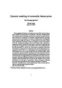
The other source of return involves a bit more explanation. In a backwardated futures market, a futures contract converges (or rolls up) to the spot price. This is the “roll yield” that a futures investor captures. The spot price can stay constant, but an investor will still earn returns from buying discounted futures contracts, which continuously roll up to the constant spot price. A bond investor might liken this situation to one of earning “positive carry.” In a contango market, the reverse occurs: an investor continuously locks in losses from futures contracts converging to a lower spot price. Correspondingly, a bond investor might liken this scenario to one of earning “negative carry.” Over very long timeframes, a number of authors have shown how the term structure of a commodity futures curve has been the dominant driver of returns in futures investing. In other words, trends in the spot price of a commodity have generally not been a meaningful driver of returns over long periods of time. In particular, Nash and Shrayer of Morgan Stanley (2004) have illustrated how over a single 21-year timeframe, the returns of a commodity futures contract have been linearly related to how backwardated the contract has been. This empirical observation is shown in Figure 5. Over the period, 1983 to 2004, the commodity futures contracts that have had the highest returns are those in which the front-month contract traded at a premium to the deferred-delivery contracts; that is, those contracts that had the highest levels of backwardation had the highest returns. Correspondingly, the contracts that have had the most negative results are those that typically traded at a discount to the deferred-delivery contracts; again, those contracts that had the highest levels of contango on average had the lowest returns. In more recent research, Feldman and Till (2006) extend the framework originated by Nash of Morgan Stanley. We find evidence that the power of backwardation to explain commodity futures returns is indeed valid, but requires the investor to have a long investment time horizon when relying on this indicator. Specifically, we examine the soybean, corn, and wheat futures markets over the period, 1950 to 2004. We find that a contract’s average level of backwardation only explains 24% of the variation in futures returns over 1-year timeframes and 39% of variation over 2-year timeframes. One must extend the evaluation period to five years, and then at that time horizon, average levels of backwardation explain 64% of the variation in futures returns. Figure 6 illustrates the latter result. Figure 7 provides a related analysis: this graph shows that over five-year time horizons, the relationship of annualized return to a contract’s average-time-inbackwardation is again highly linear. Short-term variability in commodity prices is high, which should make the spot-price return the dominant factor over shorter horizons. Over longer periods, it appears that spot commodity prices tend to be mean-reverting. This suggests that the importance of the spot return should decline as timeframes increase. The foregoing suggests that there should be a gradual increase in the fraction of futures return explained by backwardation with increasing time horizon. This relationship is similar in spirit to the increasing importance of dividend yield as a predictor of equity

7

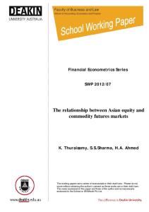
return with the lengthening of the time horizon documented by Cochrane (1999). With a one-year horizon the R-squared value of the regression of dividend yield on excess return is 17%, but at five years the R-squared value becomes 59%. These results are over the sample period, 1947 to 1996. Cochrane explains this as the result of the cumulative effects of the slight short-term predictability of a slow-moving variable. Paradigm Shift: The 1970’s Revisited As touched upon in Till (2006b), while we found that backwardation has been a driver of returns over long time horizons for three agricultural futures markets, there is another noteworthy feature of our historical results. While normally over five-year periods, an agricultural futures contract’s curve shape has been the driver of returns, there is one exception, and that is the 1970-to-1974 period. These are the data points in Figure 7 that do not fit the nearly linear trend-lines of annualized returns as a function of average backwardation. What this means for an investor is that there can be an additional fundamental rationale for a long-term, passive investment in a commodity futures contract besides predicting structural backwardation for the contract. The second rationale would be to predict that the factors are in place to repeat the 1970-to-1974 experience. For example, Howell of Schroders (2005) points out how excessive monetary stimulus had contributed to the high returns of commodities in the past. Specifically, Howell notes that negative real interest rates in the 1970’s contributed to a commodity boom at the time. And real short-term interest rates had become negative in the United States and in China during early 2005. Further, Roach of Morgan Stanley (2006) discusses the current economic environment as a “super liquidity cycle,” which is pushing the “Asset Economy to its limit,” of which one manifestation is the boom in prices of certain commodities. Now obviously one needs to be very careful about predicting trend shifts in asset prices. Grantham (2005) notes that his firm has completed research on “30 completed [asset price] bubbles … all of which came back to the pre-existing trend.” But he states, “Of these, we now believe 29 were genuine bubbles, and one – oil – was a paradigm shift …” that occurred in 1973. This is illustrated in Figure 8. Grantham, as a well-known dedicated “mean-reverter,” who underweighted Japanese equities in the late 1980’s and later underweighted U.S. technology stocks in the late 1990’s, is pausing in calling for oil to mean-revert. Even if oil becomes $80 per barrel, “given the unique features of oil, we cannot be sure it has not ratcheted up again with another trend shift.”

8

Risk Considerations Thus far, this article has focused on the drivers of returns for commodity indices and individual commodity futures contracts. This required a thorough discussion because two of the sources of return: rebalancing and roll yield are definitely not obvious. We also noted that rare trend shifts in commodity prices can also be a meaningful source of return. Another area of interest for investors is obviously the flipside of return: risk. The following section will draw from Till (2006a) in discussing portfolio-level risk considerations for an active commodity manager. This discussion will focus on risk considerations, which like the return-driver discussion, are not obvious to the neophyte in commodity investing. Risk management at the portfolio level is fundamentally different from risk management at the strategy level. At the portfolio level, an investor is concerned with how dynamic correlations among strategies may affect portfolio-level risk. An investor is further concerned with how one’s commodity portfolio may perform during financial shocks since commodity products are frequently expected to be uncorrelated to the dominant financial asset classes. This section will describe appropriate portfolio-level analyses that address these concerns. Diversified Portfolio Goal Erb and Harvey had discussed how to a large degree, commodity futures are uncorrelated with one another. A commodity portfolio manager will use this property of commodity futures contracts to attempt to create a portfolio of diversified commodity strategies with dampened risk. Commodity hedge fund manager Paul Touradji affirms this view: “One of the best things about being a commodity manager is the natural internal diversification.” “While even unrelated equities have a beta to the overall market, many commodities, such as sugar and aluminum, traditionally have no correlation at all,” according to Teague (2004) in his interview with the hedge fund manager. One difficulty with using historical correlations to evaluate portfolio risk is that correlations amongst commodities vary both seasonally and during eventful periods. There are times when a common factor can impact seemingly unrelated positions, causing a seemingly diversified portfolio to have inadvertent concentration risk to the common factor. Therefore, a commodity investor needs to include scenario analyses, which show a portfolio’s sensitivity to meaningful events, in his or her risk-measurement toolkit. Example scenario analyses are provided below. Extreme Weather Events Normally, natural gas and corn prices are unrelated. But during the summer, they can be highly correlated. During a three-week period in July 1999, for example, natural gas and corn prices were +85% correlated. Both corn and natural gas trades are heavily dependent on the outcome of weather in the U.S. Midwest. And in July, 1999, the

9

Midwest had blistering temperatures (which even led to some power outages.) During that time, both corn and natural gas futures prices responded in nearly identical fashions to weather forecasts and realizations. What this means for commodity managers is that they should measure how much sensitivity their portfolio has to extreme summer weather in the Midwest. The manager would want to ensure that in the event of a heat-wave in the U.S. Midwest that his or her portfolio would not perform exceptionally poorly. Other potentially extreme weather shocks to include in ongoing scenario analyses include the chance of an end-of-February cold shock on energy positions as well as the possibility of a damaging hurricane season in the fall. Sharp Shocks to Business Confidence Futures products are typically marketed as equity investment diversifiers. Therefore, one job of risk management is to attempt to ensure that a futures investment will not be too correlated to the equity market during periods of dramatic equity losses. Although a commodity futures portfolio may contain no financial futures contracts, the portfolio can still have systematic risk to the stock market. For example, Bessembinder (1992) found that live cattle, soybeans, silver and platinum futures contracts had statistically significant betas to the U.S. stock market using data from January 1967 to December 1989. (The data for platinum started in January 1968.) More recently, Erb and Harvey state that “the non-energy sector has a statistically significant, but small equity risk premia beta” using data from 1982 to 2004. Given the potential of a commodity portfolio to perform poorly during financial shocks, a manager should therefore examine what the portfolio’s performance would have been during the October 1987 stock market crash, the 1990 Gulf War, the Fall 1998 bond debacle, and during the immediate aftermath of September 11, 2001. If the commodity portfolio would have done poorly during these events, then the manager may consider either deleveraging his or her portfolio or buying option protection against one of the damaging scenarios. Caveat on Dynamic Correlations: The Relationship Between Commodities and Interest Rates Correlations During the Aftermath of the 9/11/01 Attacks A number of commodity futures strategies have a long commodity bias since they rely on taking on inventory risk that commercial participants wish to lay off. One consequence is that these strategies are at risk to sharp shocks to business confidence. And during sharp shocks to business confidence as occurred in the aftermath of September 11th 2001, not only did the stock market perform quite poorly, but economically sensitive commodities also performed poorly.

10

The Greenspan Federal Reserve Board had responded to financial shocks by cutting interest rates, which resulted in the stock market stabilizing. As long as this type of policy continues, one way to hedge a portfolio that has exposure to shocks to business confidence or shocks to the availability of credit is to include a fixed-income hedge. The hedge could take the form of either a Eurodollar futures contract overlay or purchases of out-of-the-money fixed-income calls. The post-9/11/01 experience validated that a long fixed-income position was an effective hedge for a portfolio that is primarily long economically sensitive commodities. Figure 9 reviews the performance of gasoline futures contracts and short-term interest rate contracts in the aftermath of the 9/11/01 attacks. While gasoline prices plummeted due to the expectation of an economic slowdown, short-term interest rate contracts rallied as the Federal Reserve Board (Fed) cut interest rates to calm the financial markets. Correlations During the Aftermath of Hurricane Katrina One caveat to this lesson is that the relationship between commodities and interest rates varies according to the type of meaningful event. For example, during the aftermath of Hurricane Katrina in late August through the middle of September 2005, gasoline and short-term interest rates reacted similarly to the prospect of scarce gasoline supplies, as shown in Figure 10. During the initial explosive rise in gasoline prices, due to the shutdown of crucial Gulf Coast refineries, interest-rate-market participants concluded that the Fed would pause in its interest-rate tightening cycle, which then caused deferred month interest-rate contracts to rally. According to a Dow Jones Newswire report (2005) of the time, “[Hurricane] Katrina shut in nearly all of oil and gas production in the Gulf of Mexico … The large scale supply disruption and fear of an economic shock triggered a massive government response. The outages prompted the Bush administration to release Strategic Petroleum Reserve oil, waive air-pollution rules on fuels, and ease restrictions on use of foreign-flagged vessels to carry fuel in U.S. waters.” Further, “Members of the Organization of Economic Cooperation and Development agreed … to [release] 2 million barrels a day of crude oil and petroleum products from their strategic stocks for 30 days.” This unprecedented government response caused gasoline prices to decline from their post-Katrina peak, and with that response, fears of an economic slump diminished, which in turn caused deferred interest-rate contracts to also decline, as the market resumed pricing in the expectation that the Fed would continue tightening interest rates. In the scenario just described, changes in daily gasoline prices and short-term interest rates became +75% correlated during the aftermath of Hurricane Katrina. This is in sharp contrast to the negative relationship between changes in gasoline prices and short-term interest rates that occurred in the aftermath of Twin Tower attacks.

11

In the aftermath of Hurricane Katrina, long positions in interest rates did not serve as an event hedge for long positions in gasoline; instead these two positions became the same trade, both on the upside and the downside. The lesson from this section is that risk management at the portfolio level is a constant and dynamic process. Final Note: Prospective Returns It is obviously useful to have a well-informed view on what the source of commodity indices’ equity-like returns were. And in addition, if one were considering an actively managed commodity program instead of an indexed investment, it is a good idea to have a well-informed view of what the sources of risk in such a program are. But clearly, what is most of interest to an investor is a prospective view of returns. At this time, the commodity index with the largest share of investor assets is the Goldman Sachs Commodity Index (GSCI). As of 11 May 2006, this index was weighted 73.4% in the energy sector. So it would likely be useful for us to examine the prospects for oil. One challenging aspect of investing in oil futures at this time is that they appear to have shifted into “structural contango.” As noted above, this means that an investor will have to absorb “negative carry” with their oil-based investments. This is analogous to investing in gold futures contracts where there has been a historical cost in synthetically paying for the storage costs of this commodity. Historically, the behavior of oil prices has been one of “structural backwardation,” consistent with the notion of crude oil inventories generally being scarce. That crude oil futures have shifted into structural contango seems to contradict the tightness that is implied by this commodity’s continuous spot price rally. What has changed? One theory from a prominent hedge fund is that the true inventories for crude oil should be represented as above-ground stocks plus excess capacity. Historically, the markets could tolerate relatively low oil inventories because there was sufficient swing capacity that could be brought on stream relatively quickly in the case of any supply disruption. This excess supply cushion has dropped to sufficiently low levels that there have been two market responses: (1) there have been continuously high spot prices to encourage either consumer conservation or the development of alternative energy supplies, and (2) the market has undertaken precautionary stock building, which has led to the steep contangos that the crude oil market has been experiencing. Stuart of UBS (2006) has examined the predicted supply and demand growth through 2010, and it appears that on trend, there will be no meaningful increase in oil spare capacity over the next four years, as shown in Figure 11. In addition the International Energy Agency (IEA) director stated, “Our impression is that the increased [oil supply]

12

capacity will just be more or less equal to the increase in demand, [with the result that] spare capacity will not increase before 2009 or 2010,” as quoted in Meir (2006). As briefly discussed in Till (2006b), in the absence of oil producers building up a spare capacity cushion and in the absence of alternative energy sources effectively replacing oil usage, the only lever to eventually balance supply and demand is demand destruction, as reasoned by Murti et al. of Goldman Sachs (2005a). The Goldman analysts examine the experience of the late 1970’s and early 1980’s to see what price spikes are required to create demand destruction and refer to their predictions as a “super spike” range. The implication of this structural change in the oil markets is that the returns to energyfocused commodity investments could become ever more long-option-like. The investor will pay away option-like premia in the form of the negative carry from the persistent contango in the oil markets, but will simultaneously be positioned for periodic (and entirely unpredictable) price spikes until an adequate supply cushion reemerges in the oil markets. That said, as Murti et al. (2005b) predict, one would expect that eventually a supply cushion will reemerge, either through behavioral changes on the part of consumers or through new infrastructure finally being constructed by producers. These changes may not occur until the end of the decade, given the very long lead time for large-scale energy projects. It is at that point one may see oil spot-prices dramatically mean-reverting, which would confirm that a curve indicator can only be expected to be useful at very long investment horizons. Conclusion This article provides a nuanced view of commodity futures investing. We discussed how commodity returns had in the past mainly relied on portfolio effects and term-structure properties of individual commodity futures contracts. But we also noted that rare trend shifts, as occurred in the early 1970’s, can also be a meaningful source of returns for a commodity investor. We further discussed some of the dynamic correlation properties of active commodity investing. These properties are also quite nuanced. Finally, we examined the prospects of the main constituent of the dominant commodity index – oil – and provided a framework for understanding what could potentially drive future returns.

13

References Bessembinder, Hendrik. “Systematic Risk, Hedging Pressure, and Risk Premiums in Futures Markets,” The Review of Financial Studies, April 1992, pp. 637-667. Dow Jones Newswire. “Nymex Crude Tumbles as Output Recovers,” 6 September 2005. Feldman, Barry and Hilary Till. “Separating the Wheat from the Chaff: Backwardation as the Long-Term Driver of Commodity Futures Performance; Evidence from Soy, Corn, and Wheat Futures Markets from 1950 to 2004,” EDHEC-Risk Publication & Premia Capital and Prism Analytics White Paper, 2006; a version of this article is forthcoming in the Journal of Alternative Investments. Cochrane, John. “New Facts in Finance,” National Bureau of Economic Research Working Paper 7169, 1999. Erb, Claude and Campbell Harvey. “The Strategic and Tactical Value of Commodity Futures,” Financial Analysts Journal, March/April 2006, pp. 69-97. Financial News Online Comment. “Turning base metals into gold,” 17 April 2006. Gorton, Gary and K. Geert Rouwenhorst. “Facts and Fantasies about Commodities Futures,” Financial Analysts Journal, March/April 2006, pp. 47-68. Grantham, Jeremy. “GMO Quarterly Letter,” July 2005. Greer, Robert. “The Nature of Commodity Index Returns,” Journal of Alternative Investments, Summer 2000, pp. 45-52. Howell, Robert. “Investment Seminar on Commodities,” Schroders Alternative Investments Group. Gstaad, February 2005. Meir, Edward and Fred Demler. Man Financial, May 2006. Meir, Edward. Man Financial Energy Daily Report, 11 May 2006. Murti, Arjun N., Brian Singer, Luis Ahn, Jonathan Stein, Ashwin Panjabi, and Zachary Podolsky. “Super Spike Period May Be Upon Us: Sector Attractive,” Goldman Sachs Global Investment Research, 30 March 2005. Murti, Arjun N., Brian Singer, Luis Ahn, Jonathan Stein, Ashwin Panjabi, and Zachary Podolsky. “Oil Bull Market in the Early Part of its Middle Phase,” Goldman Sachs Global Investment Research, 12 December 2005.

14

Nash, Daniel and Boris Shrayer. “Morgan Stanley Presentation,” IQPC Conference on Portfolio Diversification with Commodity Assets. London, 27 May 2004. Rees, Meagan. “Hermes’ Mustoe sees ‘cult of the alternative,’” Investments & Pensions Europe, 28 March 2006.

Roach, Stephen. “The Lessons of 2005,” Global Economic Comment, Morgan Stanley, 3 January 2006. Stuart, Jon. “The Fundamentally Bullish Case for Oil Stretches Through 2008, At Least,” UBS Securities Presentation, April 2006.

Teague, Solomon. “The Commodities ‘Gladiator’,” Risk Magazine, June 2004, p. 88. Till, Hilary. “Portfolio Risk Measurement in Commodity Futures Investments,” a chapter in Portfolio Analysis: Advanced Topics in Performance Measurement, Risk and Attribution (Edited by Timothy Ryan), Risk Books, London, 2006, pp. 243-262. Till, Hilary. "What the Future Holds for Commodities,” Global Alternatives Magazine, June 2006, pp. 3940.

15

Figure 1 Cumulative Value of an Investment in Commodities and US Equities (December 2001 through April 2006)

Cumulative Value of an Investment Starting with $1

3.00

2.50

2.00

1.50

1.00

D ec -0 Fe 1 b0 A 2 pr -0 Ju 2 n0 A 2 ug -0 O 2 ct -0 D 2 ec -0 Fe 2 b0 A 3 pr -0 Ju 3 n0 A 3 ug -0 O 3 ct -0 D 3 ec -0 Fe 3 b0 A 4 pr -0 Ju 4 n0 A 4 ug -0 O 4 ct -0 D 4 ec -0 Fe 4 b0 A 5 pr -0 Ju 5 n0 A 5 ug -0 O 5 ct -0 D 5 ec -0 Fe 5 b0 A 6 pr -0 6

0.50

Month Goldm an Sachs Com m odity Index - Total Return

S&P 500 Total Return Index

Data Source: Bloomberg.

Figure 2 Commodity Index Funds (in Billions of Dollars) $90 $80 Assets in Billions

$70 $60 $50 $40 $30 $20 $10 $0 90

91

92

93

94

95

96

97

98

99

'00

'01

'02

'03

'04

'05

Year

Source: Meir and Demler (2006).

16

Figure 3 Annualized Excess Returns over Treasury Bills July 1959 to December 2004 Commodity Futures 5.23 12.10 0.43

Average (%) Standard Deviation (%) Sharpe Ratio

Stocks 5.65 14.85 0.38

Bonds 2.22 8.47 0.26

Source: Gorton and Rouwenhorst (2006).

Figure 4 Annualized Return of Individual Commodity Futures Markets (April 1983 to April 2004) Annualized Return of Futures Contract (includes Interest Income) Crude Oil 15.8% 11.1% Heating Oil 18.6% Gasoline (since 1/85) Copper 12.0% Live Cattle 11.0% Corn -1.9% Wheat -0.4% Soybeans 5.7% Gold -0.2% Silver -3.3% Platinum 8.2% Soy Meal 8.8% Bean Oil 4.6% Sugar 1.8% Coffee -2.9% Cocoa -4.7% Cotton 4.1% Max Min

18.6% -4.7%

Annualized Change in Spot Price 1.1% 1.1% 3.3% 2.3% 0.7% 0.0% 0.2% 2.3% -0.5% -2.8% 3.1% 2.5% 2.9% -0.4% -2.8% -1.0% -1.1% 3.3% -2.8%

Source: Based on Nash and Shrayer (2004).

17

Figure 5 Annualized Total Return vs. Average Backwardation April 1983 to April 2004

Note: The contracts that typically trade in backwardation (gasoline, crude oil, copper, heating oil, and live cattle) had the highest average returns over the period, 1983 to 2004. Source: Nash and Shrayer (2004).

18

Figure 6 Five-Year Annualized Excess Return vs. Average Backwardation 1950 to 2004 40%

30%

Soybeans Corn Annualized 5-Year Return

20%

Wheat

Wheat Trend

Soy Trend

10%

-4.0%

-3.0%

-2.0%

-1.0%

0% 0.0%

1.0%

2.0%

3.0%

4.0%

5.0%

Corn Trend -10%

-20%

-30% Average Backwardation

Source: Feldman and Till (2006).

19

Figure 7 Five-Year Annualized Excess Return vs. Average Time-in-Backwardation 1950 to 2004

40%

30%

Soybeans Annualized 5-Year Return

20%

Corn Wheat

10%

0% 0%

10%

20%

30%

40%

50%

60%

70%

-10%

-20%

-30% Percent Time in Backwardation

Source: Feldman and Till (2006).

20

Figure 8

At Last, A Paradigm Shift New Trend from 1973

90 +2 Std Dev: 1973-2006

80

WTI Crude $ / Barrel

70 +1 Std Dev: 1973-2006

60 50 40 30

Today's Prices +2 Std Dev: 1875-1972 +1 Std Dev: 1875-1972

20

Avg.

10

01 /3 1

/1 87 01 5 /3 1/ 18 83 01 /3 1/ 18 91 01 /3 1/ 18 99 1/ 31 /1 90 7 1/ 31 /1 91 5 1/ 31 /1 92 3 1/ 31 /1 93 1 1/ 31 /1 93 9 1/ 31 /1 94 7 1/ 31 /1 95 5 1/ 31 /1 96 3 1/ 29 /1 97 1 1/ 31 /1 97 9 1/ 30 /1 98 7 1/ 31 /1 99 5 1/ 31 /2 00 3

0

Todays Prices

Average

+1 stdev

+2 stdev

-1 stdev

-2 stdev

Source: Updated from Grantham (2005).

21

Figure 9

80.0 75.0 70.0 65.0 60.0

Eurodollars (100 - Yield)

97.8 97.7 97.6 97.5 97.4 97.3 97.2 97.1 97.0 96.9 96.8

85.0

9/ 11 /2 00 9/ 1 13 /2 00 9/ 14 1 /2 00 9/ 1 17 /2 00 9/ 1 18 /2 00 9/ 19 1 /2 00 9/ 1 20 /2 00 9/ 1 21 /2 00 9/ 24 1 /2 00 9/ 1 25 /2 00 9/ 1 26 /2 00 9/ 27 1 /2 00 9/ 1 28 /2 00 10 1 /1 /2 00 10 1 /2 /2 00 1

Gasoline in Cents per Gallon

Gasoline and Short-Term U.S. Interest Rates During the Aftermath of the 9/11/01 Attacks 9/11/01 through 10/2/01

November 2001 Gasoline Contract

December 2001 Eurodollar Contract

Source: Till (2006a).

Figure 10

96.0 95.9 95.8 95.7 95.6

Eurodollars (100 - Yield)

96.1

220.0 215.0 210.0 205.0 200.0 195.0 190.0 185.0 180.0 175.0 170.0

95.5

8/ 26 /2 00 8/ 29 5 /2 00 8/ 30 5 /2 00 8/ 31 5 /2 00 5 9/ 1/ 20 05 9/ 2/ 20 05 9/ 6/ 20 05 9/ 7/ 20 05 9/ 8/ 20 05 9/ 9/ 20 0 9/ 12 5 /2 00 9/ 13 5 /2 00 9/ 14 5 /2 00 9/ 15 5 /2 00 9/ 16 5 /2 00 5

Gasoline in Cents per Gallon

Gasoline and Short-Term U.S. Interest Rates Around the Time of Hurricane Katrina End-August through Mid-September 2005

Novem ber 2005 Gasoline Contract

March 2006 Eurodollar Contract

Source: Till (2006a).

22

Figure 11 Spare Capacity Growth of Next to Nothing Through 2010

Source: Stuart (2006).

23