PSYCHOMETRIKA--VOL.56, NO. 2, 327-348 JUNE 1991
STATISTICAL
INFERENCE
FOR MULTIPLE
CHOICE
TESTS
JOHN S.J. H s u DEPARTMENT OF STATISTICS AND APPLIED PROBABILITY THE UNIVERSITY OF CALIFORNIA, SANTA BARBARA TOM LEONARD
KAM-WAH Tsui DEPARTMENT OF STATISTICS THE UNIVERSITY OF WISCONSIN, MADISON Finite sample inference procedures are considered for analyzing the observed scores on a multiple choice test with several items, where, for example, the items are dissimilar, or the item responses are correlated. A discrete p-parameter exponential family model leads to a generalized linear model framework and, in a special case, a convenient regression of true score upon observed score. Techniques based upon the likelihood function, Akaike's information criteria (AtC), an approximate Bayesian marginalization procedure based on conditional maximization (BCM), and simulations for exact posterior densities (importance sampling) are used to facilitate finite sample investigations of the average true score, individual true scores, and various probabilities of interest. A simulation study suggests that, when the examinees come from two different populations, the exponential family can adequately generalize Duncan's beta-binomial model. Extensions to regression models, the classical test theory model, and empirical Bayes estimation problems are mentioned, The Duncan, Keats, and Matsumura data sets are used to illustrate potential advantages and flexibility of the exponential family model, and the BCM technique. Key words: multiple choice test, exponential family, likelihood, Akaike's information criterion, generalized linear model, Bayesian marginalization, importance sampling, regression of true score upon observed score, classical test theory model.
1.
Introduction
W e c o n s i d e r a p r o b l e m h i g h l i g h t e d b y L o r d a n d N o v i c k (1968, p. 524), D u n c a n (1974), a n d M o r r i s o n a n d B r o c k w a y (1979). S u p p o s e that a n e x a m i n e e c o m p l e t e s a m u l t i p l e c h o i c e t e s t w i t h m i t e m s and o b t a i n s y c o r r e c t r e s p o n s e s o u t o f m. T h e n a n u m b e r o f a p p e a l i n g c h o i c e s , s u c h as t h e c o m p o u n d b i n o m i a l e r r o r m o d e l ( L o r d & N o v i c k , p. 384), a r e a v a i l a b l e f o r m o d e l i n g the r a n d o m v a r i a b i l i t y o f y. N o t e t h a t
y = x i + '''
+ Xm,
(1)
w h e r e X l , . . . , x m a r e b i n a r y r e s p o n s e s , w i t h x l = 1 if the e x a m i n e e c o r r e c t l y a n s w e r s t h e i-th i t e m , a n d x i = 0 o t h e r w i s e . O n e a p p r o a c h is to first m o d e l t h e j o i n t p r o b a b i l i t y mass function p(xl, x2 ..... x , n ) o f Xl, . . . , X m . S e v e r a l p o s s i b i l i t i e s are i. T h e b e t a - b i n o m i a l m o d e l ( D u n c a n , 1974; L e o n a r d & N o v i c k , 1986; P r e n t i c e & The authors wish to thank Ella Mae Matsumura for her data set and helpful comments, Frank Baker for his advice on item response theory, Hirotugu Akaike and Taskin Atilgan, for helpful discussions regarding AIC, Graham Wood for his advice concerning the class of all binomial mixture models, Yiu Ming Chiu for providing useful references and information on tetrachoric models, and the Editor and two referees for suggesting several references and alternative approaches. Requests for reprints should be sent to John S.J. Hsu, Department of Statistics and Applied Probability, University of California-Santa Barbara, Santa Barbara, CA 93106. 0033-3123/91/0600-89181 $00.75/0 © 1991 The Psychometric Society
327
328
PSYCHOMETRIKA
Barlow, 1988). Suppose that the items are similar or parallel and that x 1, . . . , x m are permutable. Given s¢, take x l , • • • , Xm to be independent and binary distributed with common probability ~:. Then, if ¢ possesses a beta distribution, y in (1) possesses a beta-binomial distribution. Therefore, a mixture of binomial distributions for y can always be justified by a permutable (i.e., exchangeable) distribution for x l . . . . , X m . The beta-binomial model may also be reasonable for y in some situations where x 1. . . . , x m are not permutable. ii. A m o d i f i e d b e t a - b i n o m i a l m o d e l (Morrison & Brockway, 1979). In model i, let ~:= s¢* + c(l - (*), where c is a guessing parameter and ~ possesses a beta distribution. Then the distribution of y may be expressed as a finite series. iii. A m u l t i v a r i a t e l o g i s t i c ~ b i n a r y d i s t r i b u t i o n (Anderson & Aitken, 1985; Leonard, 1972). Suppose that, given ¢1 . . . . , era, the random variables x l , . • • , Xm possess binary distributions with respective probabilities S ~ l , . . . , Cm, and consider the logits ~'i = log ~i - - log(1 - ~ i ) . Take ~'1. . . . . ~m to possess a multivariate normal distribution. Then appropriate choices of the covariances introduce flexible interdependencies between x l . . . . , x m. Also, unequal means or unequal variances permit the modeling of dissimilar items. The true score may be defined as ~t + " " " + ~:m,and it is in principle possible to predict the true score, for any particular examinee. However, it is difficult to express the distribution of y in closed form, and any analysis would require heavy computations. iv. G e n e r a l m i x t u r e s (Bock & Aitken, 1981 ; Hsu, 1990; Leonard, 1984; Lord, 1969; Lord & Novick, I988, p. 512; Lord & Stocking, 1976). In Model i, take s¢ to possess cumulative distribution function G where, for example, G may be estimated as a discrete distribution, using generalized maximum likelihood procedures. If the user is less interested in modeling the joint distribution ofx~ . . . . , xm, a more direct approach may be developed by assuming the distribution of y to belong to a family that is broad enough to approximate, as special cases, the compound binomial error model, the beta-binomial model, the modified beta-binomial model, the generalized hypergeometric model (Keats, 1964), the gamma-Poisson model (Wilcox, 1981a, 1981b), the four-parameter beta-binomial model (Lord, 1965), the beta-binomial mixture model (Bell, 1990; Dalai & Hall, 1983), and the distributions o f y in Models iii and iv. Other generalizations of the simple binomial model were discussed by Consul (1974, 1975), Altham (1978), Lord (1965), and Carter and Williford (1975). For a review, see Wilcox (1981a). A very general specification of discrete distributions is provided by the discrete p-parameter exponential family (e.g., Leonard, Hsu, & Tsui, 1989, Takane, Bozdogan, & Shibayama, 1987), which assumes that_.~_~j = p ( y = J3 satisfies eVJ
q~j = - - ,
(j = O, 1. . . .
, m),
(2)
m
Z e~/h h=O
where the multivariate logits To, 3q, • • •, Tm are linear functions, Tj = aj + 01bl(j)
+ 02b2(j)
+''"
+ Opbp(j),
(3)
of specified basic functions a j , b l ( j ) , b2(j), . . . , bp(j3; O1 . . . . . Op are unknown parameters, and p < m is either specified or unknown. We will proceed under the particular assumptions aj = log m
Cj,
( j = O, 1 . . . .
, m),
(4)
JOHN S.J. HSU, TOM LEONARD, AND KAM-WAH TSUI
329
where m c j = rn!/j!(m - j ) ! , and bk(j) =
, (k = 1, . . . , p; j = 0, 1, . . . , m),
(5)
so that we have a polynomial model for the logits, in the spirit of Bock (1972) and others. When p = 1, y possesses a binomial distribution with probability e°l/(1 + e °l) and sample size m. However, a larger value ofp permits substantial deviations from the binomial distribution. When p = 2, a two parameter distribution, similar in quality to the beta-binomial distribution is obtained. However, another reasonable choice is p = 4, since the quartic function in (3) then permits bimodality of the probability mass function of y, and hence, the potential for a reasonable fit to many data sets. An appropriately large choice ofp will enable us to approximate many previously proposed procedures for modeling the distribution of y. The polynomials in (5) can be replaced by a variety of other convenient choices of basis function, such as B-splines or terms from a Fourier Series. The usual p-dimensional minimal sufficient statistic, when p is fixed, can always be expressed as the vector of the corresponding sample quantities, and we can refer to standard exponential family theory for estimation (e.g., Lehmann, 1983, p. 80). For example, for fixed p, there always exist sufficient statistics that are uniform minimum variance unbiased estimators of their expectations, a finite sample property. The model in (2) through (5) will permit the prediction of an average true score, across a set of examinees. As it is not described in two stages, it does not in general facilitate the prediction of individual true scores. When the items are dissimilar, a model of the complexity of Model iii or the tetrachoric correlation model (Lord & Novick, p. 345), would be required to express individual true scores as sums of m components corresponding to the different items. Nevertheless, in the special case where the model in (2) through (5) approximates a model of the form of Model iv for some cumulative distribution function G, it is possible to predict individual true scores. This key property is described below in comment (iv) and (12). Suppose that n examinees respectively score y ] , . . . , Yn correct responses out of m. Then, if Yl . . . . , Yn are independent, the likelihood of 0' = (01, • • •, Op), given Y' = ( Y l , . . . , Yn), under assumptions (2) through (5), is !(01, . . . ,
Op; PlY)= exp {to + 0 1 t l + ' ' '
+ Optp -nA(0)},
(6)
where m
to = X
(7)
ajnj,
j=0
and the (fixed p) minimal sufficient statistics tl, • • . , tp
tk = ~
nj
, (k= I,...,
satisfy
p),
(81
j=l
with nj representing the number of examinees with score j, and m
A(0) = log ~'~ exp {aj + m - l O l j j=0
+ m - 2 0 2 j 2 + • • • + rn-POpjP}.
(9)
330
PSYCHOMETRIKA
The explicit parameters in the exponential family model are not always meaningful in their own right, since the model is motivated toward a reasonable semi-parametric fit to the data. However, many parameters of interest can be expressed as functions of the model parameters, and our objective is to make finite sample inferences about the parameters of interest. In section 2 we will consider maximum likelihood procedures for 01 . . . . , Op together with an information criterion (e.g., Akaike, 1978; Atilgan & Leonard, 1988). In section 4 we will discuss more precise finite sample inference for parameters of interest that are arbitrary functions of 01,. • •, Op, for example: (i). The s a m p l e m e a n or a v e r a g e true score. m
j=l m
= ~ j exp {aj + m - l O l j + . . .
+ m - P O p j p - A(O)}.
(lO)
(ii). The probability o f passing. ~7 = p ( y >-- a) m
= E 6i j=a m
E
exp {aj + m - I O l j + • • • + m - P O p j p - A(0)},
(11)
j=a
where a denotes the passing score. (iii). C o m p a r i s o n o f t w o groups. We will consider the probability that the score Yl of a randomly chosen examinee from one group exceeds the score Y2 of a randomly chosen person from another group. (iv). Individual true scores. Whenever the model in (2) through (5) is equivalent to a general mixture of the form described in Model iv (the results by Lord, 1969, tell us that this may sometimes, but not always, be exactly true or approximately true), the conditional expectation of the logit 7 = log ~ - log(1 - 0, the binomial mixture model, given y, is 0 log 4~y
2/* = E(ylY) =
Oy
+ tk(y + I) - 0(m - y + 1)
(12)
= O l m -1 + 2 0 2 m - 2 y + 3 0 3 m - 3 y 3 + • . . + p O p m - P y v - l ,
where ~ y) = 0 log F(y)/0y denotes the digamma function. The digamma terms conveniently vanish because of assumption (4). Hence, a particular examinee's true ability, given observed score, can be predicted by ¢'* = eV*/(1 + er*), where 7* is the linear function of 01, . . . , Op defined in (12). Then ¢'* is much more general than the linear regression of ~ on y predicted by the beta-binomial model. Although Lord (1969) indicates that, for any observed score distribution, the true score distribution is not uniquely defined, the value of ~* will be unaffected by this choice. Equation (12) provides an alternative to the regression of true score on observed score, considered by
331
JOHN S.J. HSU, TOM LEONARD, AND KAM-WAH TSUI
L o r d and Novick (1968, p. 513). The predictive variance of % given y, is just the first derivative with respect to y of (12) and this will be positive whenever the two models are identical. In this case, the first p predictive moments may be obtained by further differentiations, and predictive central moments higher than the first p are zero. The full result in (12) seems new; see Appendix 1 for details of our derivation, and section 8 for an analogue within the framework of the classical test theory model. Until recently, the nonlinear functions in (10) and (11) would have created severe technical difficulties. H o w e v e r , these will be circumvented via recent developments in Bayesian marginalization (e.g., Geweke, 1988, 1989; Leonard, 1982; and Leonard, Hsu, & Tsui, 1989), which permit a precise finite sample analysis of complicated nonlinear models with several parameters. 2.
Likelihood Techniques
When p is specified, the likelihood (6) may be analyzed within the standard framework of generalized linear models (McCullagh & Nelder, 1985, p. 142). The maximum likelihood estimates hi, • • • , Op of 01, • • • , Op, for fixed p, satisfy the equations
tk = n
j
, (k= 1,...
,p),
(13)
m - P O p j p - A(0)},
(14)
j=l
where the tk satisfy (8), and (~j =
exp {(aj
+ m-lOlj
+ • "" +
and the likelihood information matrix R of 01, • • •, Op has elements rkk. satisfying k+k*
j(1-
(k= 1,...,
p; k* = 1 , . . . ,
p).
(15)
j=l
The matrix R also provides the Hessian in the Newton-Raphson iterations for the maximization of the log of the likelihood (6) and the existence of a finite solution is guaranteed for nonzero t l , . . . , tp. Then 0 = ( h i , . . . , Op)' yields consistent point estimation for 0 = (01, • • • , Op)' as n ---) 0% with p fixed, and for finite n, (13) provides uniform minimum variance unbiased estimators for p linear functions of ~bI , . . . , 4)m . Also, as n ~ ~, with p fixed, Rl/2(ti - 0) converges in distribution to a standard multivariate normal distribution. Hence, the likelihood dispersion matrix R - l may be regarded as a large sample estimated covariance matrix for ti, and approximate confidence intervals for linear combinations of 0 are available. When p is unspecified, one possibility is to choose p to maximize the general information criterion (GIC) GIC = L p - 21 a p ,
(16)
where L p is the log of the likelihood (6), evaluated at the maximum likelihood estimates, and oLdenotes a penalty per parameter included in the model. Various choices of a have been proposed (e.g., Akaike, 1978, Atilgan, 1983, and Schwarz, 1978). For example, a = 2, and a = log n respectively lead to Akaike's information criterion AIC = L p - p , and Schwarz's information criterion
(17)
332
PSYCHOMETRIKA 1
BIC = Lp - ~p log n.
(18)
Alternatively, if Lp is plotted as a function of p, then the graph typically rises rapidly for small p, and then flattens into a slightly increasing ridge. The problem is to estimate a sensible value for p near the beginning of the ridge. One possibility is Atilgan's empirical information criterion (EIC) that considers the vertices P l, P2 . . . . of the convex boundary of the plot of Lp against p, and then chooses the vertex minimizing "YiPi, where Yi is the slope of the convex boundary after the i-th vertex. Atilgan performs simulations to show that AIC and the data dependent EIC typically perform equally well, and somewhat better than other choices of a. As a preliminary to the Bayesian analysis of Section 4, we recommend evaluating p by AIC, since a mixed model analysis is much more complicated. Akaike (1978) provides a Bayesian justification for this preliminary step, by assuming a particular prior distribution for p. These ideas are easy to extend to further regression situations, thus providing an alternative to the beta-binomial developments of Prentice and Barlow (1988). Suppose we have n observed scores Yl, • • -, Yn with corresponding design points Ul, • • -, Un. Then let the i-th observation possess the distribution defined in (2) through (5), but with 01 replaced by, say/3 o + / 3 1 U i . The p + 1 parameters /3o, /31, 0 2 . . . . , Op may be estimated within the generalized linear model framework, and 02 , . . . , Op measure the deviations from the standard linear logistic model for binomial data. The term 02j 2 -tOpjp can be interpreted as a "parametric residual" in the sense of Leonard and Novick (1986). A more complicated regression component, or dependence of 02, . . . , 0p on the design points, can also be considered. •
•
•
q-
3.
Simulation Results
Five hundred simulations were first performed, where on each simulation n = 200 1 B (0.4,10) + 2 B(0.6,10) of two observations were generated from a mixture 13 binomial distributions, with mixing probabilities ~ and ~, binomial probabilities 0.4 and 0.6, and common sample size ra = 10. On each simulation, we fitted a beta-binomial distribution, with parameters estimated by maximum likelihood, and the exponential family distribution in (2) through (5), with p = 2. The exponential family distribution fitted the data, with a lower value of the chi-squared goodness-of-fit statistic X2, with eight degrees of freedom, on 349 out of the 500 simulations. The average value of X2, under the exponential family model, was 22 = 8.623, compared with 22 = 8.828 under the beta-binomial model. The fitted exponential family model was closer to the true model, when compared with the beta-binomial model, on 424 out of the 500 simulations. Here, we measured the distance from the true model by DEVIANCE =
m (j~ _ ej)2 ~ > , j=0 ej
(19)
where ej is the fitted frequency for thej-th cell, under the fitted model, and3~ family is the expected frequency under the true model. The average deviance of 2.517 for the exponential family model was less than the corresponding value of 2.761 for the betabinomial model. A further 500 simulations were performed, each generating n = 200 observations from the 0.4B(0.3,10) + 0.6B(0.8,10) mixture. On each simulation, a beta-binomial distribution was compared with the exponential family distribution, with p = 4. The latter yielded a much lower value for the normalized chi-squared statistic )(2/6, when compared with the statistic )(2/8, for the beta-binomial distribution, on each of the 500
333
J O H N S . J . H S U , TOM L E O N A R D , A N D K A M - W A H TSUI
simulations. The average ~:2 = 8.604 compared with an average ~:2 = 41.501 for the beta-binomial model. The exponential family model was closer to the true model on each of the 500 simulations, when an average deviance of 6.376 compared with an average deviance of 34.486 for the beta-binomial model. Hence, there do exist situations where the generality of (2) through (5) may prove useful when compared with other models. 4.
Bayesian Marginalization
In some situations it may be possible to incorporate prior information regarding 0 = (01, • • •, 0p)' via a multivariate normal prior distribution, say with mean vector Ixo and covariance matrix C 0. For example, Co could be taken to represent the covariance structure of an autoregressive process in the spirit of Young (1977) and Leonard (1973). It may be valuable to incorporate prior information when p is large, to obtain smoother estimates, but this is less important when p is small, when the parameters are better estimated by the data. This formulation provides a flexible alternative to the prior mixture of beta distributions recommended by Dalai and Hall (1983) and Bell (1990) for binomial models. The posterior density of 0 for fixed p, is, using the notation of section 1,
7r(01y)
~ exp { O l t l + ' ' "
+ Optp -- nA(0) - ~(0
[Jl.o)}, (0 E R P ) . (20) However, as tC01 -> o% the prior information becomes vague, and quadratic term, within the exponential of (20), vanishes, and (20) becomes proportional to the likelihood (6). In general, we consider a parameter of interest ~l=g(O)=g(01,
...
-
~ll,0)'col(0
, Op), (~1 ~
fl),
-
(21)
without further regularity conditions concerning g, where ll denotes the set of possible values of 7. Special cases include the average true score (10) and probability of success (11). The marginal posterior density of 71is
~'(nly) = lira 8-1 fD 7r(0ly)d0, (77 E f t ) ,
(22)
8---, 0
where D denotes the region D = O(r/, 6) = { 0 : 7 / < 9 ( 0 ) < ~/ + 6},
(23)
and ~0ly) satisfies (20). The integration in (22) is difficult to exactly perform, unless p is small. However, an approximation fully described by Leonard, Hsu, and Tsui (1989) referred to here as BCM (Bayesian conditional maximization) typically gives precise results (see Appendix 2 for details). BCM involves three components, including the maximized posterior density
•r u ( n l y ) =
sup
~'(0ty), (~7 ~ fl),
(24)
0:g(0) = n
which conditionally maximizes (20) subject to the constraint (21). For the functions in (10) and (I I), it is straightforward to compute (24), and the conditional maximum On, of 0, given 77, using standard Newton-Raphson/Lagrange multiplier methods. However (24) does not generally approximate (22) as well as possible. The adjustment terms described by Leonard et al. (1989) each merit inclusion. A key adjustment term, for
334
PSYCHOMETRIKA
finite samples, depends upon the density f(r/lix, C) of r/ = g(0) when 0 possesses a multivariate normal distribution with mean vector IXand covariance matrix C, where Ix and C are particular functions of On. For the functions in (10) and (11), further approximations to J'(~711~, C) are required. For (10), f was approximated by taking ,1/rn to possess a beta distribution with correct first two moments, obtained by computer simulation. For (I 1), a similar beta approximation was used for r/. If instead 71 = ~bj for some fixed j, we have
= ~J = 1 + ej(O)'
(25)
where
ej(O) = ~ exp h~j
( a h -- a j +
m - l O l ( h --j) + m - 2 0 2 ( h 2 _j2) + "" " + m - P O p ( h
p -jP)}.
(26)
In this case, the density of ej(O) was first approximated by a log-normal density, with correct first moments, and the transformation (25) used to obtain ourfcontribution for 71. Note that the moments of (26) can be obtained analytically if 0 possesses a multivariate normal distribution. Secondly, a scale multiple of F-approximation was used, with correct first three moments, for ej(O) and again referred to the transformation (25). As an alternative to the BCM procedure, it is possible to simulate the exact posterior density of 71in (22) using importance sampling (e.g., Geweke, 1988, 1989; Leonard et al., 1989; Rubinstein, 1981). In the present context we recommend simulating 0 vectors from a multivariate normal distribution with mean vector 0 and covariance matrix D, where 0 unconditionally maximizes (20) and D-1 denotes the Hessian in the Newton-Raphson iterations for the unconditional maximum. As Ic01 ~ ~, is just the maximum likelihood vector satisfying (13), and D -1 is just the likelihood information matrix R, whose elements satisfy (15). Then importance sampling (see Rubinstein, 1981, for details) permits simulation of the exact posterior density (22), even though the simulations for 0 are from an approximate distribution. The Gibbs sampler (e.g., Gelfand & Smith, I990) could be used to try to speed up the convergence, but this is not particularly necessary for the current straightforward model. Hsu (1990) considers a discrete mixture of binomials as an alternative to our exponential family model. Unfortunately, the regularity conditions for BCM breakdown for the discrete binomial mixture model owing to multimodality of the likelihood function. Hsu develops a generalization of importance sampling (referred to as permutable Bayesian marginalization, PBM) for handling discrete mixtures. However, BCM for our exponential family model is much simpler when compared with PBM for the binomial mixture model. Note that BCM is also applicable to the models considered by Mislevy (1986), as an alternative to procedures based upon joint posterior modes. 5.
The Duncan Data
We first analyze the Duncan data (Duncan, 1974, p. 55; Morrison & Brockway, 1979, p. 439) that consists of two random samples, from a discrete distribution for the observed number of successful responses on m = 20 items. For the likelihood analysis of section 2, AIC was minimized in both cases when p = 2, and EIC provided similar results. The maximum likelihood estimates of 01 and 02, together with their approximate standard errors (in brackets), obtained via (15), are reported in Table 1, for the
335
JOHN S.J. HSU, TOM LEONARD, AND KAM-WAH TSUI
TABLE 1 M a x i m u m L i k e l i h o o d A n a l y s i s for D u n c a n D a t a
Group 1
~x
~2
X~0
AIC
-17.78
22.94
2.35
-2545.93
12.76
-1960.03
(2.94) (2.39) Group 2
-18.90
23.77
(3.22)
(2.64)
two groups of examinees. Note that 01 and 02 are more than five standard errors from zero in each case, refuting a simple binomial model (02 = 0). Our calculations of the chi-squared statistic on ten degrees of freedom is based on a similar grouping of the cells to the grouping employed by Morrison and Brockway. The values X20 = 2.35 and 12.76 are similar to the values of 2.01 and 12.56 obtained by Morrison and Brockway for Duncan's beta-binomial model, and the values X92 = 1.82 and 12.82 obtained for their modified beta-binomial model. However, under our model, it is easier to obtain approximate confidence intervals by reference to the likelihood dispersion matrix R -l , where R has elements defined in (15). As our parameter space is a subset oflogit space, there is good potential for approximate normality. For the two groups of the Duncan data, the likelihood dispersion matrices are (8.616-6.925)
(10.378-8.380)
R -j =
, and R -1 = - 6.925
5.714
. - 8.380
6.954
In this case, (12) reduces to a linear regression of true score on observed score. Consider the predicted true score, in logit space, 3'* =
01 + 1.202 20
,
(27)
for an examinee who correctly answers y = 12 items out of 20. Then, in the two groups, 3'* has maximum likelihood estimates 0.4874 and 0.4812, with approximate standard errors 0.0236 and 0.0264, yielding approximate 95% confidence intervals (0.4401, 0.5337) and (0.4295, 0.5329) for 3'*. The corresponding maximum likelihood estimator of ~ = e ~ are 0.6195 and 0.6180, quite close to the observed score of 0.6, with reassuringly narrow 95% intervals (0.6083, 0.6303) and (0.6058, 0.6301). In this case, the predictive variance of 3' given y is 02/200 and this has maximum likelihood estimates 0.1147 and 0.1189 in the two groups, with standard errors 0.012 and 0.013 I. More precise and detailed inferences are available under the Bayesian paradigm (see Figures I-6). Only figures for the first group of examinees are reported here; similar results are available for the second group of examinees. Figure 1 describes the posterior density of 02 , for the first group of examinees, and under the uniform prior for 0 = (Oi, 02)' obtained by letting IC01---> ~. Histogram (a) used 50,000 simulations for the
336
PSYCHOMETRIKA
(a) !
(b)
to
(c)
m 0
0 0
Ihll 1/3 0
-
0
I
I,I!
I
0 d
-
I
I
15
20
I
I
25
30
FIGURE l
Posterior density of 02 (group 1). (a) histogram; (b) maximized posterior density; (c) BCM. importance sampling technique discussed in section 4. Curve (b) is the maximized posterior density (24), but renormalized to integrate to unity. Curve (c) was obtained by the BCM techniques of section 4. When 7/= Oj for some j , BCM reduces to Laplace's method (Leonard, 1982) which does not involve an f-contribution. Note the reassuringly close correspondence between the approximate and simulated exact results. As the posterior density of 02 is strongly concentrated on the region (0, 00), this confirms that a binomial model (02 = 0) is inappropriate. As the posterior density is slightly skew to the left, a normal approximation is not quite adequate. In Figure 2, we describe similar curves but for the predicted true score C described above. In Figure 3, we consider inferences for r; = ~b20, the probability of correctly
337
JOHN S.J. HSU, TOM LEONARD, AND KAM-WAH TSUI
(a) (b) (c)
0 CO
0 "d"
0 04
0
I
I
i
I
I
I
!
0.59
0.60
0.61
0.62
0.63
0.64
0.65
FIGURE 2 Posterior density of an examinee predicted true score when she/he correctly answered 12 items (group l). (a) histogram; (b) maximized posterior density; (¢) BCM.
answering all 20 items, which possesses maximum likelihood estimates ~b20 = 0.00185 and 4)20 = 0.00198 in the two groups. The two BCM curves (c) and (d) compare favorably with the normalized maximized posterior density (b) in relation to the simulated histogram (a). Curves (c) and (d) follow the two different suggestions made in section 4 for the e-contribution to (25). Curve (c) uses a log-normal, and curve (d) uses a scale multiple of F-contribution. The posterior mean of ~b20 is equal to 0.00190; this is our Bayes estimate under squared error loss and also our predictive probability that a further student answers all 20 items correctly. In Figure 4, we assume that a student passes the test if he correctly answers 12
338
0 0
PSYCHOMETRIKA
--
\ 0 0
--
0 0
--
0 0 (,')
--
0 0 C~
-
. . . .
(a) (b)
.............
(d)
(c)
\ \ \ \ 0 0
-
0
--
\ kx
I
I
0.0
0.002
I.......
0.004
l
I
0.006
0.008
FIGURE 3 Posterior density of 4~0 (group 1). (a) histogram; (b) maximized posterior density; (c) BCM with lognorma! contribution; (d) BCM with a scale multiple of F contribution.
items, so that , / = t~l 2 + " " " + t~20 is the probability o f passing. The BCM c u r v e (c), for ~ in (11) includes an f-contribution corresponding to a beta density with correct first two moments, and improves upon the normalized maximized posterior density (b), when compared with Histogram (a). The posterior means/predictive probabilities o f success, for the two groups, were 0.646 and 0.635, compared with maximum likelihood estimates o f 0.650 and 0.642. In Figure 5, we consider the posterior densities of the average true score (10). In this case the BCM curve (c) was very close to the normalized maximized posterior density (b). The posterior means of the average true score were respectively 12.48 and
339
JOHN S.J. HSU, TOM LEONARD, AND KAM-WAH TSUI
(a) (b) (c)
0
_
tt)
0
-
-
I
I
I
I
I
0.55
0.60
0.65
0.70
0.75
FIGURE 4 Posterior density of probability of passing (group 1). (a) histogram; (b) maximized posterior density; (c) BCM.
12.28, providing optimal predictions under squared error loss, and comparing with maximum likelihood estimate of 12.56 and 12.51. Finally, Figure 6 permits formal comparisons of the results for the two groups by considering ~ = P(Yl < Y2) and 7?2 = P(Yl > Y2), again w i t h p = 2, where Yl and Y2 are the observed scores, for randomly selected examinees from groups 1 and 2. Histograms (a) and (b) describe our simulated posterior densities for ~71 and 92, while (c) and (d) providing corresponding smooth curves obtained via a version of BCM (technical details omitted). The maximum likelihood estimates hi = 0.450 and $/2 = 0.458 compare with posterior means of 0.451 and 0.458. Since $/1 < $/2, this suggests that examinees from Group 1 are slightly more likely to perform better than examinees from Group 2.
340
PSYCHOMETRIKA
(a) (b) (c)
143
0
0
0 d
-
I
I
I
I
I
11.5
12.0
12.5
13.0
13.5
FIGURE 5 Posterior density of (average) true score (group 1). (a) histogram; (b) maximized posterior density; (c) BCM.
6.
The Matsumura Data
In Table 2 we report the observed scores for 145 University of Wisconsin Accounting students, each of whom completed 4 tests, the first three tests containing 25 dissimilar items, and the last test containing 30 dissimilar items. We fitted the exponential family model, using the techniques described in section 2. The AIC criterion suggested p = 3 for Test A, and p = 2 for each of tests B, C, and D. For Test A, our value of chi-squared was X62 = 7.09, with six degrees of freedom (based on the 10 groupings 0-16, 17, 18 . . . . . 25 of the items) and this was comparable with a betabinomial fit that provided X72 = 7.37, with seven degrees of freedom.
JOHN S.J. HSU, TOM LEONARD, AND KAM-WAHTSUI
341
(a),(c) (b),(d)
04 ',1'-' .
.
.
.
.
.
.
.
.
.
.
.
.
O
O0
tJD
i
--
V '¢t"
-
Cq
-
0
--
I
I
I
0.30
0.35
0.40
"I ..................
0.45
I
I
I
0.50
0.55
0.60
FIGURE6 Comparison of two groups. (a) histogram for p(yl < Y2); (b) histogram for p(yl > Y2); (c) BCM for p(yl < Y2); (d) BCM for p(y I > Y2). The maximum likelihood estimates b 1 = 167.82, b2 = -215.73 and 03 = 112.4I, for Test A, possessed respective approximate standard errors 100.66, I25.83, and 51.9. This yields, from (12), the quadratic regression, 7* = 6.713 - 0.690y + .0215y 2. T h e deviation o f 03 from zero can be more accurately judged by reference to Figure 7. Histogram (a) describes our simulated posterior density for 03, under uniform priors for 01 , 02, and 03 , and curve (c) describes our BCM approximation. The posterior density is skew to the right and the value 03 = 0 lies in the extreme left tail. Therefore, the Bayesian analysis makes it quite evident that the cubic term should be included in the sampling model. Standard techniques for generalized linear models do not permit such precise judgments concerning individual parameters.
O0
GO
~
"q
O~
~
~
0
0
CO
¢,o
¢,o
CD
~
0
0
t~
0
0
0
0
0
0
0
0
C?
0
r~
©
0 ~,.,°
0
©
t~
©
0
t~
o
el
343
JOHN S.J. HSU, TOM LEONARD, AND KAM-WAH TSUI O0 0 0 0
(a) .... (0 0 0 0
-
~I" 0 0 0
-
(b) (c)
L"M O O O
-
o
(:5 I
I
I
0
50
100
!
I
I
I
150
200
250
300
FIGURE 7
Posterior density of 03 (Matsumura's EXAM A). (a) histogram; (b) maximized posterior density; (c) BCM. The remainder of our analysis of the Matsumura data is omitted for brevity of presentation. We however, finally mention the data described by Leonard et al. (1989, sec. 7) where n = 200 and m = 10, with n 0, n I . . . . , nl0 respectively equalling 8, 12, 17, 18, 12, 23, 27, 34, 31, 14, and 4. In this case, our model with p = 3 fitted well with X72 = 5.59, comparing favorably with the beta-binomial fit, g 2 = 19.23. 7.
The Keats Data
Columns 1 and 2 o f Table 3 present the observed frequency distribution reported by Keats (1964). We fitted the exponential family model, using the techniques described in section 2. The AIC criterion suggested p = 5. The maximum likelihood estimates
344
PSYCHOMETRIKA
TABLE 3 Comparison of Observed Distribution with Four Estimated Distributions Four-
Five-
Parameter
Parameter
Raw
Observed
Beta-
Quadratic
Gamma-
Exponential
Score
Frequency
Binomial
Regression
Poisson
Family
0
0
0.26
2.43
0.79
0.06
1
0
0.63
2.05
0.97
0.37
2
1
1.10
2.10
1.18
1.06
3
2
1.66
2.29
1.44
2.07
4
4
2.30
2.56
1.75
3.15
5
6
3.02
2.91
2.14
4.11
6
7
3.82
3.34
2.60
4.87
7
2
4.71
3.87
3.17
5.44
8
3
5.69
4.52
3.85
5.92
9
4
6.77
5.29
4.67
6.40
10
5
7.96
6.22
5.67
6.95
11
14
9.26
7.34
6.87
7.67
12
10
10.70
8.68
8.32
8.61
13 14
12 10
12.28 14.03
10.29 12.21
10.05 12.13
9.87 11.51
15
14
15.98
14.51
14.62
13.63
16 17
17 16
18.16 20.61
17.25 20.52
17.58 21.10
16.31 19.64
18
22
23.40
24.41
25.25
23.69
19
27
26.61
29.02
30.14
28.50
20
37
30.37
34.46
35.85
34.11
21
48
34.86
40.84
42.47
40.53
22
40
40.40
48.25
50.06
47.80
23
50
47.58
56.77
58.64
56.01
24
74
57.54
66.39
68.14
65.36
25
78
72.30
76.96
78.37
76.09
26
85
94.17
88.07
88.84
88.39
27
103
121.46
198.76
98.58
101.79
28
112
139.28
107.05
105.68
113.48
29
114
119.00
108.58
106.09
114.25
30
83
54.05
92.04
89.44
82.38
JOHN S.J. HSU, TOM LEONARD, AND KAM-WAH TSUI
345
48.56, 02. = 14.68, 03 = 217.30, 04 = 259.14, and 05 = 112.26. Our value of chi-squared was X~8 = 14.91, with 18 degrees of freedom (based on 24 groupings 0-5, 6--8, 9, 1 0 , . . . , 30 of the items) and the chi-square level of significance was 0.67, and these were comparable with the four-parameter beta-binomial model, the quadratic regression model suggested by Keats (1964) and the gamma-Poisson model suggested by Wilcox (1981a, 1981b) provided chi-squared values X29 = 45.91, X29 = 21.30, and )(21 = 26.87 with degrees of freedom 19, 19 and 21 and chi-square levels of significance were 0.0005, 0.32, and 0.18, respectively. The corresponding estimated frequency distributions are presented in columns 3--6 in Table 3. The exponential family model produced larger chi-square level of significance than the other three models in this example. A Bayesian analysis of the Keats data is also available from the authors.
w e r e b I -=
8.
The Classical Test Theory Model
Consider the classical test theory model (Lord & Novick, 1968, p. 56), X = T + E,
(28)
where X is the observed score and T is the true score. Suppose that T and E are independent and the E is normally distributed with mean zero and known variance o-2. Then the regression of true score upon observed score is E(TIX)=X+o
0 log p(X) -2 - , OX
(29)
where p(x) denotes the unconditional density of x. Suppose also that the density of X belongs to the continuous p-parameter exponential family p(x) = exp {01 tl (x)
- O(a)},
+ 02t2(x ) +" '' + Optp(X)
( - o o < x < oo),
(30) where D(0) = log J_= exp {Oltl(x) + 02t2(x) + • • • + Optp(X)} dx.
(31)
Then (29) reduces to the regression E(TIX) = X + o.2(01tl 1) (x) + 202t(21) (x) + ' ' " + pOp,p .(1) (x)),
(32)
where tJ 1) (x) = Otj(x) OX
'
for j = l
2,...,p.
(33)
Most of the techniques described in our paper are readily generalizable to this model. There are obvious applications of (12) and (32) to empirical Bayes estimation problems for binomial and normal data (e.g., Leonard, 1972, 1984; Lord, 1969). 9.
Concluding Remarks
Our exponential family model provides a framework for handling dissimilar items and inhomogeneous populations of students (e.g., the Keats data) and will often be more flexible than the simple beta-binomial model and its generalizations. It explains
346
PSYCHOMETRIKA
many data sets without needing the construction of a guessing parameter, depending upon the item, rather than upon the student's abilities and knowledge. Note that the simple beta-binomial model possesses a coefficient of variation larger than does a binomial model with the same mean. On many data sets where the items are dissimilar (e.g., the Keats data), the coefficient of variation is smaller than for a binomial model with the same mean. Trying to explain this by an extra guessing parameter, rather than a more appropriate sampling model might be quite misleading. Of course, if the guessing probability for any particular item is constant and non-zero across all students, then Morrison and Brockway (I979) introduce the guessing aspect into the standard betabinomial model, in a simple, appealing and estimable manner, providing an advantage when compared with the exponential family formulation. However, Wilcox (1981a, p. 22) discusses three further problems involving guessing parameters. With appropriate choices o f p and the basis functions b l , b 2 , • • • , bp in (3), most practical data sets, requiring generalizations of random sampling from the binomial distribution, can be modelled by a member of the p-parameter exponential family, defined by (2) and (3), and our approach may therefore be regarded as global in nature. It might be reasonable to use our approach to explore the main features of the data, but, to use our analysis to suggest a specialized model from the literature, for example, the Morrison-Brockway model, or one of the alternatives cited in section 1, for confirmatory purposes. Appendix 1 We give fuller details of property (iv) of section I, and the derivation of (I 2). Under the beta-binomial model, ~bj = p ( y = j) takes the form ~ j = rnfjE[~J(1 _ ~ ) m - j ]
= m C j E [(1 Jr : ~ / '
(j = 0, 1 ....
, m),
3'
where the first expectation is with respect to some distribution for ¢, and the second expectation is with respect to a corresponding distribution of 3' = log ~: - log(1 - ¢3. Therefore, 0 log 4~r -=-&(y+ 0y
1)+ ~b(m-y+ 1)+
E[7(1 + e3") - m exp (y~/)] 3" E[(1 + eV) -m exp (y),)] 3"
= - O ( y + 1) + ~O(m - y + 1) + E ( y l y ) , yielding E(~,Iy) =
0 log (~y t- ~b(y + 1) - ~b(m - y + 1). ay
The result so far is reasonably standard. However, when ~bj also satisfies (2) through (5), for some 01, • • •, Op, appropriate differentiations of log qSy yield (12) together with the further results stated in property (iv) of section I.
JOHN S.J. HSU, TOM LEONARD~ AND KAM-WAH TSU1
347
Appendix 2 We now describe fuller details of the BCM procedure discussed in section 4. Leonard, Hsu, and Tsui (1989) obtain this via a Taylor Series expansion of the log posterior density log ~01Y) about the conditional maximum On. If the cubic and higher terms are neglected, then the following apparently extremely accurate approximation to (22) can be obtained analytically: lr*(r/lY) ~ ~rM(rllY)f(~lO*, R n t ) f * ( ~ ) ,
(n ~ D.),
where 1. ~rM(nly) is the maximized posterior density satisfying (24); 2. f(~[ix, C) denotes the density of r / = g(0) when 0 has a multivariate normal distribution with mean vector Ix and covariance matrix C; 3. if(r/) = exp with a. R n = -[(02 log ~r(OlY))/0(OO')]0=0,, denoting the posterior information matrix of 0, evaluated at the conditional maximum 0 n; b. e.~ = [(0 log 7r(O[y))/O0]0=o,;
IR,1-1/2
c. 0 n
(~e'nRne,),
0 n + R~len.
Further computations or approximations for the f contribution f(rllIx, C) are typically required. The results in the current paper suggest that any sensible approximation, capturing the first two moments, will probably suffice. References Akaike, H. 0978). A Bayesian analysis of the minimum AIC procedure. Annals of the Institute of Statistical Mathematics, 30(A), 9-14. Altham, P. M. E. 0978). Two generalizations of the binomial distribution. Applied Statistics, 27, 162-167. Anderson, D. A., & Aitken, M. (1985). Marginal maximum likelihood estimation of item parameters: Application of an algorithm. Journal of Royal Statistical Society, Series B, 26,203-210. Atilgan, T. (1983). Parameter parsimony, model selection, and smooth density estimation. Unpublished doctoral dissertation, University of Wisconsin-Madison. Atilgan, T., & Leonard, T. (1988). On the application of AIC to bivariate density estimation, non-parametric regression, and discrimination. In H. Bozadogan & A. K. Gupta (Eds.), Multivariate statistical modeling and data analysis (pp. 1-16). Dordrecht, Holland: Reidel. Bell, S. S. (t990). Empirical Bayes alternatives to the beta-binomial model. Unpublished doctoral dissertation, Columbia University. Bock, R. D. (1972). Estimating item parameters and latent ability when responses are scored in two or more nominal categories. Psychometrika, 37, 29-51. Bock, R. D., & Aitken, M. (1981). Marginal maximum likelihood estimation of item parameters: application of an EM algorithm. Psychometrika, 46, 443-454. Carter, M. C., & Williford, W. O. (1975). Estimation in a modified binomial distribution. Applied Statistics, 24, 319-328. Consul, P. C. (1974). A simple urn model dependent upon predetermined strategy. Sankhya, Series B, 36, 391-399. Consul, P. C. (1975). On a characterization of Lagrangian Poisson and quasi-binomial distributions. Communications in Statistics, 4, 555-563. Dalai, S. R., & Hall, W. J. (1983). Approximating priors by mixtures of natural conjugate priors. Journal of Royal Statistical Society, Series B, 45,278-286. Duncan, G. T. (1974). An empirical Bayes approach to scoring multiple-choice tests in the misinformation model. Journal of the American Statistical Association, 69, 50--57. Gelfand, A. E., & Smith, A. F. M. (1990). Sampling based approaches to calculating marginal densities. Journal of the American Statistical Association, 85, 398-409. Geweke, J. (1988). Antithetic acceleration of Monte-Carlo integration in Bayesian inference. Journal of Econometrics, 38, 73--89.
348
PSYCHOMETRIKA
Geweke, J. (1989). Exact predictive density for linear models with arch distributions. Journal of Econometrics, 40, 63-86. Hsu, J. S.J. (1990). Bayesian inference and marginalization. Unpublished doctoral dissertation, University of Wisconsin-Madison. Keats, J. A. (1964). Some generalizations of a theoretical distribution of mental test scores. Psychometrika, 29, 215-231. Lehmann, E. L. (1983). Theory of point estimation. New York: John Wiley & Sons. Leonard, T. (1972). Bayesian methods for binomial data. Biometrika, 59, 581-589. Leonard, T. (1973). A Bayesian method for histograms. Biometrika, 60, 297-308. Leonard, T. (1982). Comment on the paper by Lejeune and Faulkenberry. Journal of the American Statistical Association, 77, 657-658. Leonard, T. (1984). Some data-analytic modifications to Bayes-Stein estimation. Annals of the Institute of Statistical Mathematics, 36, 11-21. Leonard, T., Hsu, J, SJ., & Tsui, K. (1989). Bayesian marginal inference. Journal o f the American Statistical Association, 84, 1051-1058. Leonard, T., & Novick, J. B. (1986). Bayesian full rank marginalization for two-way contingency tables. Journal o f Educational Statistics, 11, 33--56. Lord, F. M. (1965). A strong true-score theory, with applications. Psychometrika, 30, 239-270. Lord, F. M. (1969). Estimating true-score distributions in psychological testing: An empirical Bayes estimation problem. Psychometrika, 34, 259-299. Lord, F. M., & Novick, M. R. (1968). Statistical theories of mental test scores (with contributions by Allen Birnbaum). Reading, MA: Addison-Wiley. Lord, F. M., & Stocking, M. L. (1976). An interval estimate for making statistical inference about true scores. Psychometrika, 41, 79-87. McCullagh, P., & Nelder, J. A. (1985). Generalized linear models. New York: Chapman and Hall. Mislevy, R. J. (1986). Bayes modal estimation in item response. Psychometrika, 51, 177-195. Morrison, D. G., & Brockway, G. (1979). A modified beta-binomial model with applications to multiple choice and taste tests. Psychometrika, 44, 427-442. Prentice, R. L., & Barlow, W. E. (1988). Correlated binary regression with covariates specific to each binary observation. Biometrics, 44, 1033--48. Rubinstein, R. Y. (1981). Simulation and the Monte Carlo method. New York: John Wiley and Sons. Schwarz, G. (1978). Estimating the dimension of a model. Annals of Mathematical Statistics, 6, 461--464. Takane, Y., Bozdogan, H., & Shibayama, T. (1987). Ideal point discriminant analysis. Psychometrika, 52, 371-392. Wilcox, R. R. (1981a). A review of the beta-binomial model and its extensions. Journal o f Educational Statistics, 6, 3-32. Wilcox, R. R. (1981b). A cautionary note on estimating the reliability of a mastery test with the beta-binomial model. Applied Psychological Measurement, ~, 531-537. Young, A. S. (1977). A Bayesian approach to prediction using polynomials. Biometrika, 64, 309-318.
Manuscript received 11/6/89 Final version received 6/6/90