Remediation by steam injection Jacob Gudbjerg

Remediation by steam injection

Ph.D. Thesis, October 2003

Jacob Gudbjerg Environment & Resources DTU Technical University of Denmark

Remediation by steam injection Cover: Birte Brejl Printed by: DTU tryk Environmental & Resources DTU ISBN 87-89220-74-9 The thesis will be available as a downloadable pdf-file from the department's homepage on: www.er.dtu.dk Environment & Resources DTU Library Bygningstorvet, Building 115, Technical University of Denmark DK-2800 Kgs. Lyngby Phone: Direct (+45) 45 25 16 10 (+45) 45 25 16 00 Fax: (+45) 45 93 28 50 E-mail: [email protected]

2

Preface The present report “Remediation by steam injection” has been submitted as a part of the requirements for the Ph.D. degree at the Technical University of Denmark. The study has been performed at Environment & Resources DTU in the period April 2000 to July 2003, with Karsten Høgh Jensen and Torben Obel Sonnenborg as supervisors. The report consists of a review followed by four journal papers where the first one has been published and the last three have been submitted for publication. Reinhard Schmidt performed the experimental work in the first paper and part of the numerical work was performed during my master’s project. Oliver Trötschler and Arne Färber performed the 2-D experiments in the third paper. The review will mainly focus on the issues I have worked with during my study and as such should not be regarded as a complete review of all the research that has been performed concerning steam injection. In chronological order I would like to thank the following people. First of all, Kent Udell for starting my interest in steam injection. Since his very inspiring lecture at the Technical University of Denmark in the autumn of 1998 not a single day has passed where I have not thought about steam injection. Hopefully, that is going to change. I want to thank Reinhard Schmidt for letting me use his excellent data sets and for the good cooperation we had during the making of our paper. I am grateful to the people at the VEGAS-facility at the University of Stuttgart for letting me use their excellent experimental facilities and for the technical support they provided during my stay there. I also want to thank Gorm and Tom Heron, Thomas Hauerberg Larsen, Jarl Dall Jepsen, Torben Højbjerg Jørgensen and Hans Skou for keeping me in contact with real-life applications of steam injection. That has kept me focused on the important issues and prevented me from getting lost in unimportant details.

The following institutions provided the necessary funding for the study: Danish Environmental Protection Agency, Programme for Development of Technology - Soil and Groundwater Contamination Groundwater Research Center, DTU Danish Energy Authority, Energy Research Programme.

The papers are not included in this www-version but can be obtained from the Library at Environment & Resources DTU, Bygningstorvet, Building 115, Technical University of Denmark, DK-2800 Lyngby ([email protected]). Lyngby, October 2003 Jacob Gudbjerg 3

Abstract Chemical spills have created a large number of contaminated sites where toxic compounds are present as nonaqueous phase liquids (NAPL). These sites have proved difficult to remediate and aggressive technologies are needed. Remediation by steam injection is such a technology and it may be the optimal technology at heavily contaminated sites. Steam injection involves the injection of steam into the subsurface and simultaneous recovery of fluids from extraction wells. The injected steam heats the soil and creates a steam zone that expands from the injection wells as more steam is injected. The physical-chemical properties of typical contaminants change with temperature and this makes them easier to extract. In particular the increase in vapor pressure is important. Additionally, two immiscible liquid phases will boil when the sum of their vapor pressures equals the surrounding pressure and this phenomenon proves very important for the contaminant mass transfer. The objectives of this study have been to further our understanding of the dominant processes and mechanisms involved in steam injection through the use of numerical modeling, laboratory experiments and field-scale data. The focus has been on the following four issues that have been reported separately: 1. Removal of NAPLs from the unsaturated zone using steam: prevention of downward migration by injecting mixtures of steam and air Steam injection for remediation of porous media contaminated by nonaqueous phase liquids has been shown to be a potentially efficient technology. There is, however, concern that the technique may lead to downward migration of separate phase contaminant. In this work a modification of the steam injection technology is presented where a mixture of steam and air was injected. In two-dimensional experiments with unsaturated porous medium contaminated with non-aqueous phase liquids it was demonstrated how injection of pure steam lead to severe downward migration. Similar experiments where steam and air were injected simultaneously resulted in practically no downward migration and still rapid cleanup was achieved. The processes responsible for the prevention of downward migration when injecting steam-air mixtures were analyzed using a non-isothermal multiphase flow and transport model. Hereby, three mechanisms were identified and it was demonstrated how the effectiveness of these mechanisms depended on the air to steam mixing ratio.

2. Remediation of NAPL below the water table by steam induced heat conduction Previous experimental studies have shown that NAPL will be removed when it is contacted by steam. However, in full-scale operations steam may not contact the NAPL directly and this is the situation addressed in this study. A two-dimensional intermediate scale sand box experiment was performed where an organic contaminant was emplaced below the water table at the interface between a coarse and a fine sand layer. Steam was injected above the water table and after an initial heating period the contaminant was recovered at the outlet. The experiment was successfully modeled using the numerical code T2VOC and the dominant removal mechanism was identified to be heat conduction induced boiling of the separate phase contaminant. Subsequent numerical modeling showed that this mechanism was insensitive to the 4

porous medium properties and that it could be evaluated by considering only onedimensional heat conduction. 3. On spurious water flow during numerical simulation of steam injection into water saturated soil Numerical simulation of steam injection into a water saturated porous medium may be hindered by unphysical behavior causing the model to slow down. We show how spurious water flow may arise on the boundary between a steam zone and a saturated zone, giving rise to dramatic pressure drops. This is caused by the discretization of the temperature gradient coupled with the direct relation between pressure and temperature in the steam zone. The problem may be a severe limitation to numerical modeling. A solution is presented where the spurious water flow is blocked and this widely enhances the performance of the model. This new method is applied to a previously reported example exhibiting numerical problems. Furthermore, it is applied to the simulation of 2-D sand box experiments where LNAPL is remediated from a smearing zone by steam injection. These experiments would have been difficult to analyze numerically without the adjustment to prevent spurious flow. The simulation proves to be very sensitive to the type of relative permeability model. The LNAPL is removed by a combination of vaporization and flow. Based on the numerical results it is argued that it is necessary for the steam to contact the NAPL directly to achieve clean-up at field-scale. 4. Three-dimensional numerical modeling of steam override observed at a fullscale remediation of an unconfined aquifer Steam injected below the water table tends to move upwards because of buoyancy. This limits the horizontal steam zone development, which determines the optimal spacing between injection wells. In this study, observations indicating steam override at a full-scale remediation of an unconfined aquifer are analyzed by numerical modeling using the code T2VOC. A simplified 3-D numerical model is set up, which qualitatively shows the same mechanisms as observed at the site. By means of the model it is found that it will be possible to achieve a larger horizontal extent of the steam zone in a layered geology compared to the homogeneous case. In the homogeneous case the steam injection rate increases dramatically when the injection pressure is increased, which is necessary to achieve a larger horizontal development. The development of the steam zone under unconfined conditions is found to be a complex function of the geologic layering, the ground water table at steady-state extraction and the injection/extraction system. Because of this complexity it will be difficult to predict steam behavior without 3-D numerical modeling.

5

Resume Spild af kemikalier har skabt et stort antal forurenede grunde, hvor toksiske forbindelser er til stede som fri fase. Det har vist sig vanskeligt at oprense disse grunde, og det er nødvendigt at benytte aggressive oprensningsteknologier. Oprensning ved dampinjektion er en sådan teknologi, og det kan være den optimale teknologi ved kraftigt forurenede grunde. Ved dampinjektion injiceres damp i undergrunden samtidig med, at der oppumpes i ekstraktionsbrønde. Den injicerede damp opvarmer jorden og skaber en dampzone, som ekspanderer væk fra injektionsbrønden, efterhånden som mere damp injiceres. De fysisk-kemiske egenskaber for typiske forureningsstoffer ændrer sig med temperaturen, og det gør dem lettere at ekstrahere. Specielt er stigningen i damptryk meget vigtig. Ydermere vil to ikke-blandbare væsker koge, når summen af deres damptryk svarer til omgivelsernes tryk, og dette fænomen vises sig at være meget vigtigt for transporten af forurening. Formålet med dette projekt har været at øge forståelsen af de dominerende processer og mekanismer i dampinjektion gennem numerisk modellering, laboratorieforsøg og data fra en oprensning på felt-skala. Fokus har været på de følgende fire emner som er blevet afrapporteret særskilt: 1. Fjernelse af fri fase fra den umættede zone ved hjælp af damp: forhindring af nedadrettet transport ved injektion af damp-luft blandinger Dampinjektion til oprensning af porøse medier forurenet med ikke-vandig fri fase har vist sig at være en potentiel effektiv teknologi. Der er dog bekymring for, at teknikken kan føre til nedadrettet transport af forurening på fri fase. I dette projekt præsenteres en modifikation af teknikken, hvor en blanding af damp og luft blev injiceret. I to-dimensionale eksperimenter med umættet porøst medium forurenet med fri fase blev det demonstreret, hvordan injektion af ren damp førte til nedadrettet transport. Tilsvarende eksperimenter, hvor damp og luft blev injiceret samtidig viste stort set ingen nedadrettet transport, og stadigvæk blev hurtig oprensning opnået. De dominerende processer for forhindringen af nedadrettet transport ved damp-luft injektion blev analyseret ved hjælp af en ikke-isoterm flerfasestrømning og transport model. Herved blev tre mekanismer identificeret, og det blev vist hvordan effektiviteten af disse mekanismer afhang af damp-luft blandingsforholdet. 2. Oprensning af fri fase under grundvandsspejlet ved damp-induceret varmeledning Tidligere eksperimentelle studier har vist, at fri fase bliver fjernet, når den kommer i kontakt med damp. I oprensninger på fuld skala kan damp dog ikke altid komme i direkte kontakt med den fri fase, og den situation er emnet for dette projekt. Et to-dimensionalt forsøg i en kasse med sand blev udført, hvor en organisk forurening blev placeret under grundvandsspejlet på grænsefladen mellem et groft og et fint sandlag. Damp blev injiceret over grundvandsspejlet og efter en initial opvarmningsperiode blev forureningen ekstraheret ved udløbet. Forsøget blev simuleret tilfredsstillende ved hjælp af den numeriske model T2VOC og den dominerende fjernelsesmekanisme blev identificeret som kogning af den frie fase forårsaget af varmeledning. Efterfølgende numerisk modellering viste, at denne mekanisme ikke var sensitiv over for det porøse mediums egenskaber, og at den kunne evalueres ved kun at betragte en-dimensional varmeledning. 6

3. Om falsk vandstrømning ved numerisk simulering af dampinjektion i vandmættet jord Numerisk modellering af dampinjektion i vandmættet porøst medium kan blive hæmmet af ufysisk opførsel, som får modellen til at køre langsomt. Vi viser, hvordan falsk vandstrømning kan opstå på grænsen mellem en dampzone og en mættet zone, hvilket giver anledning til dramatiske trykfald. Det er forårsaget af diskretiseringen af temperaturgradienten sammenholdt med den direkte relation mellem tryk og temperatur i en dampzone. Problemet kan være en alvorlig begrænsning for numerisk modellering. En løsning bliver præsenteret, hvor den uægte vandstrømning blokeres, hvilket øger modellens ydelse betragteligt. Denne nye metode bliver anvendt på et tidligere afrapporteret eksempel, der udviste numeriske problemer. Ydermere bliver den anvendt til at simulere to-dimensionale eksperimenter, hvor fri fase blev oprenset ved dampinjektion. Disse eksperimenter ville have været svære at analysere numerisk uden justeringen til at forhindre falsk vandstrømning. Simuleringen viser sig at være meget sensitiv over for typen af relativ permeabilitetsmodel. Den frie fase blev fjernet ved en kombination af fordampning og strømning. Baseret på de numeriske resultater argumenteres der for, at det er nødvendigt med direkte kontakt mellem damp og den frie fase for at kunne oprense på fuld skala. 4. Tre-dimensional numerisk modellering af dampoverløb observeret ved en fuld-skala oprensning af et frit grundvandsmagasin. Damp injiceret under grundvandsspejlet vil bevæge sig opad på grund af opdrift. Det begrænser den horisontale udbredelse af dampzone, som bestemmer den optimale afstand mellem injektionsboringerne. I dette projekt bliver observationer, der indikerer dampoverløb ved en fuld-skala oprensning af et frit grundvandsmagasin analyseret ved numerisk modellering med modellen T2VOC. En forsimplet tredimensional model bliver opsat, som kvalitativt viser de mekanismer, der blev observeret på grunden. Ved hjælp af modellen findes det, at det vil muligt at opnå en større horisontal udbredelse af dampzonen i en lagdelt geologi sammenlignet med det homogene tilfælde. I det homogene tilfælde stiger dampinjektionsraten dramatisk, når injektionstrykket øges, hvilket er nødvendigt for at opnå større horisontal udbredelse. Udviklingen af dampzonen i et frit magasin er en kompleks funktion af den geologiske lagdeling, grundvandsspejlet ved oppumpning og injektions/ekstraktionssystemet. På grund af den kompleksitet vil det være vanskeligt at forudse dampens opførsel uden tre-dimensional numerisk modellering.

7

Table of contents Table of contents ............................................................................................................8 1. Introduction............................................................................................................9 1.1. Temperature effect on physical-chemical properties...................................10 1.2. Steam injection.............................................................................................11 2. Objectives.............................................................................................................12 3. Numerical modeling.............................................................................................13 3.1. Governing equations ....................................................................................13 3.2. Capillary pressure ........................................................................................15 3.2.1. Temperature dependence of capillary pressure....................................16 3.3. Relative permeability...................................................................................18 3.4. Hysteresis .....................................................................................................20 3.5. Implementation of the BC capillary pressure-saturation model ..................21 3.5.1. Verification ..............................................................................................23 3.6. Unphysical simulation results ......................................................................25 4. Removal mechanisms ..........................................................................................29 4.1. Frontal removal............................................................................................29 4.2. Conduction-induced boiling.........................................................................30 4.3. NAPL flow...................................................................................................33 4.4. Additional mechanisms................................................................................33 5. Steam zone development .....................................................................................34 5.1. 1-D steam zone development .......................................................................34 5.2. 3-D steam zone development .......................................................................34 5.2.1. Unsaturated zone..................................................................................35 6. Downward migration ...........................................................................................37 7. Future research areas............................................................................................39 7.1. Cyclic injection............................................................................................39 7.2. Steam injection in fractured systems ...........................................................39 7.3. Temperature effect on capillary pressure.....................................................39 8. Conclusions ..........................................................................................................40 9. References ............................................................................................................41

8

1. Introduction Industrial activities during the last four to five decades have created a large number of sites where chemical spills have contaminated the subsurface. It is estimated that 14,000 sites in Denmark are contaminated due to spills (Danish EPA 1999). Contamination is basically found where chemicals have been used in large amounts and typically below old gas stations, dry cleaners, military bases, gas works etc. Typical contaminants are chlorinated solvents, gasoline/fuels, coal tar and creosote. These contaminants are almost immiscible with water and will often be present as nonaqueous phase liquids (NAPL). Mercer and Cohen (1990) provide the following description of NAPL transport in subsurface. When spilled into the unsaturated zone the NAPL migrates downward due to gravity. The NAPL may spread horizontally due to capillary forces and heterogeneities and furthermore some of the NAPL may be immobilized as residual. If the spill is large enough the NAPL eventually reaches the saturated zone where it floats in the top of the capillary fringe if it is lighter than water (LNAPL) and migrates further downwards if it is denser than water (DNAPL). Low permeable layers in the saturated zone may arrest the downward migration and divert the flow horizontally or pools may form in depressions. Entrapment will also occur in the saturated zone and usually at a higher saturation than in the unsaturated zone. LNAPL may also become entrapped in the saturated zone due to water table fluctuations during which an LNAPL smearing zone is formed. The transport of NAPL is influenced by heterogeneities at all scales and therefore extremely difficult to predict and furthermore the heterogeneous distribution makes it difficult to detect and quantify a given spill. The NAPL in the subsurface may evaporate into the gas phase and spread in the unsaturated zone and dissolved components will spread with the water phase. Even though the solubility is low it is much higher than common drinking water standards. This means that even a small spill can potentially contaminate large groundwater resources and it may take very long time before the NAPL is completely dissolved. In addition to the contamination of the groundwater, chemicals in the gas phase may migrate into housing. Because of the risk of human exposure to these chemicals combined with their toxicity it may be necessary to remediate a contaminated site. This is most often done by excavating the contaminated soil and treating it off site. However, at some sites the volume of contaminated soil might be too large or there might be buildings that make it impossible to excavate. Therefore remediation has to take place in situ without disturbing the soil. Traditional in situ remediation technologies are pump-and-treat in saturated zone and soil vapor extraction in the unsaturated zone. Unfortunately, these technologies have shown to be very inefficient at NAPL sites. The mass transfer rate from the heterogeneously distributed NAPL becomes diffusion-limited and large volumes need to be flushed to achieve clean-up. Furthermore, Sale and McWhorther (2001) showed that near-complete removal of NAPL is necessary to reduce the short-term groundwater concentration. At heavily contaminated sites the clean-up time may be in the order of decades with these technologies. Consequently, there is a need for more aggressive technologies that can address these sites effectively. Innovative technologies have been proposed such as surfactant flooding, alcohol flooding, chemical oxidation and air sparging; however, these technologies may also be limited by diffusion and the efficiency can be strongly 9

influenced by heterogeneities. Thermal technologies provide a means to overcome these limitations and may in some case be able to achieve clean-up goals rapidly. With thermal technologies the contaminated soil is heated and this strongly affects the physical-chemical properties of the contaminants in most cases to the benefit of the recovery process. This is the fundamental basis of thermal technologies and the most important temperature effects will be briefly described here.

1.1.

Temperature effect on physical -chemical properties

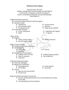
The vapor pressure increases dramatically with temperature (Fig. 1) and this is the most important reason why thermal technologies are effective. As the vapor pressure increases the contaminant will vaporize into the gas phase, where it is much easier to remove than in the water phase or as a NAPL. Water TCE TCE + water

Vapor pressure [kPa]

120

Atmospheric pressure 80

40

0 0

20

40 60 Temperature [°C]

80

100

Fig. 1. Vapor pressure as a function of temperature for water, TCE and the sum (Reid et al. 1983).

At 100 °C the vapor pressure of water is equal to the atmospheric pressure, which is marked by the horizontal line in Fig. 1. This is by definition the normal boiling point. When two immiscible liquids are present their vapor pressures will be independent and the liquids will boil when their summed vapor pressure equals the atmospheric pressure (Atkins, 1996). Thus, the boiling point for two immiscible liquids will be lower than both their individual boiling points. This intuitively surprising result will show to be extremely important for the mass transfer from the NAPL phase. The viscosity decreases with temperature making NAPL flow more rapid; however, remediation rarely relies on NAPL flow alone and the viscosity reduction is therefore of little importance. Flow of NAPL will always leave a residual phase behind and a reduction in ground water concentration will only be achieved at the very long term. The density of NAPL and water decreases slightly with temperature but not enough to significantly affect the flow processes. The solubility of contaminants generally increases with temperature. Heron et al. (1998) found a 15 % increase in the solubility of TCE from 7 °C to 71 °C. This, of 10

course, makes it easier to extract contaminant in the water phase; however, removal in the water phase will still be extremely slow. Sorption decreases with increasing temperature (Sleep and McClure 2001b) and where the removal is limited by sorption this may be significant. Still, only little contaminant mass can be sorbed compared to the mass present as NAPL. Thus, the increased mass removal because of a decrease in sorption is not expected to justify a full-scale steam thermal operation. Diffusion increases with temperature but still diffusion will not affect the mass removal significantly. Generally speaking the temperature effect on the physical-chemical properties make the contaminants more mobile and thereby easier to remove; however, it is the effect on the vapor pressure that justifies the use of thermal technologies for remediation.

1.2.

Steam injection

Steam injection is the most commonly used thermal remediation technology. It involves the injection of steam into subsurface combined with extraction in the water, gas and NAPL phases. As previously stated it is the increase in vapor pressure that is important in thermal technologies and therefore contaminants will mainly be extracted in the gas phase. Extraction of the water phase is mostly performed to avoid spreading of contaminant. When steam contacts the soil it condenses and heats the soil. A zone with steam temperature is formed, which expands as more steam is injected. This process and the actual contaminant removal mechanisms will be addressed later. Steam injection was originally developed as an enhanced oil recovery technology where it was the reduction in viscosity that was most important. Oil in reservoirs has a much lower viscosity than typical contaminants and often the vapor pressure is too low to be considered. Therefore the scope has been somewhat different and in this particular study steam injection as an oil recovery technique will not be addressed or very much referenced. That being said, it is obvious that much of the pioneering work on steam injection as a remediation technology was based on the experiences from steam injection as an enhanced oil recovery technique. The technology is expensive and difficult to implement and should only be used in highly contaminated source zones where rapid remediation is required.

11

2. Objectives The overall objectives of this study have been to further our understanding of the dominant mechanisms involved in remediation by steam injection. An increased understanding will help us to apply the technology in the most optimal way. The approach has been to use numerical modeling combined with laboratory experiments and data from field-scale applications. This has resulted in four journal papers, which addresses different aspects as reflected by their titles: 1) Removal of NAPLs from the unsaturated zone using steam: prevention of downward migration by injecting mixtures of steam and air 2) Remediation of NAPL below the water table by steam induced heat conduction 3) On spurious water flow during numerical simulation of steam injection into water saturated soil 4) Three-dimensional numerical modeling of steam override observed at a fullscale remediation of an unconfined aquifer The first part of the thesis presents a brief review of the current status of steam injection as a remediation technology. This is not a comprehensive review of all the work that has been done within this field but rather a review of the current understanding of the dominant processes and mechanisms. Thus, only key studies that illustrate these processes and mechanisms are referenced. A second objective of this document is to provide a more thorough description of the numerical model, as this has been the most essential tool in this study. In that description some of the preliminary considerations that lead to the approaches taken in the papers are described.

12

3. Numerical modeling The numerical code used in this study T2VOC (Falta et al., 1995) is a member of the TOUGH family of codes developed to simulate multidimensional, non-isothermal, multiphase flow and transport in porous media (Pruess, 1987; Pruess, 1991).

3.1.

Governing equations

This section briefly describes the governing equations of the T2VOC code. The description is largely based on the T2VOC User’s Guide (Falta et al., 1995). The model considers gas, water and NAPL as separate phases. These phases consist of the three components air, water and chemical. As an example a gas phase may be a mixture of air, water and chemical or in the case of pure steam it would be only water. Note the difference between water as a component and water as a phase. In non-isothermal mode heat is considered a fourth component. For each of the components a balance equation is formulated: d M κ dVn = ∫ F κ ⋅ n dAn + ∫ q k dVn (1) dt V∫n An Vn where M is the mass or energy of component κ (air, water, chemical or heat) per unit porous medium volume Vn , Fκ is the flux of κ through the surface area An of Vn and qκ is the mass or heat generation per unit volume. The mass/energy term is calculated as a sum of the contributions from the separate phases: M κ = φ ∑ S β ρ β X κβ (2) β

where φ is porosity, S is saturation and ρ is density of phase β and X is the mass fraction of component κ in phase β. For the component heat the mass fraction is replaced by the specific internal energy and the specific internal energy of the soil grains is added. For the chemical an additional term may be added to include sorption. The flux term is calculated as the sum of advection/convection and diffusion/conduction where the former is calculated by a multiphase extension of Darcy’s law: k rβ ρ β κ κ Fadvection/ (∇Pβ − ρ β g ) (3) convection = ∑ − X β k µβ β where k is the intrinsic permeability, krβ is the relative permeability to phase β, ρ is the density, µ is the viscosity, P is the pressure and g is the gravitational acceleration vector. In the case of heat flux the mass fraction is once again replaced by the specific internal energy. Mass flux by diffusion is included in the gas and water phase through Fick’s law: κ Fdiffusion = ∑ − φ S β D κβ ρ β ∇ X κβ (4) β

κ β

where D is the molecular diffusion coefficient of κ in the β phase. Diffusion in the water phase is actually not described in the T2VOC User’s manual and has not been included in the presented simulations. However, it is now part of the new release of T2VOC. Heat flux by conduction is calculated from Fourier’s law: 13

Fconduction = − K∇T (5) where K is the overall heat conductivity coefficient of the porous medium. The mass/ heat generation term q in equation (1) may represent various forms of sinks and sources such as fluid injection or withdrawal. The model assumes equilibrium among the phases within each gridblock and the component distribution is calculated from functions relating vapor pressure and solubility to temperature. Water dissolved in the NAPL phase is not accounted for. The set of equations are discretized by integral finite difference technique, which is illustrated in Fig. 2.

Fig. 2. Integral finite difference discretization. From Falta et al. (1995).

Fnm is the flux from gridblock m with the volume Vm across the interface Anm into gridblock n with the volume Vn . The flux is calculated from the finite differences between for instance phase pressures in the gridblocks and the distance Dm + Dn . Thus, a gridblock is defined by a volume and the connections to other gridblocks. The connections are again defined by a contact area and a distance from the center to the contact area. In this type of discretization the gridblocks can have any size and any shape and do not have to be related to any physical position. Generally, upstream weighting is used except that the heat conductivity coefficient is harmonically weighted and the density in the calculation of the gravity contribution is arithmetically averaged. Other weighting schemes may be applied and for instance Gudbjerg et al. (2003a) changed the upstream weighting factor for the density of the water phase to ρ ij = 0.98ρi + 0.02ρ j , where i is the upstream gridblock This greatly improved the stability of the model when a NAPL phase had just disappeared from a gridblock. The non-linear algebraic equations are solved by Newton-Raphson iteration and the linear equations arising from this are solved by iterative preconditioned conjugate gradient techniques. The four mass balance equations are solved for four independent primary variables. Since the three phases may not be present in all gridblocks at all times it is necessary to switch between different sets of primary variables for each phase combination. The model assumes that the water phase is always present and consequently there are four possible phase combinations as listed in Table 1. 14

Table 1. Phase combinations and primary variables.

Phases Primary variables Water Pwater Xair-water T χchemical-water Water, NAPL PNAPL Swater Xair-water T Water, gas Pgas Swater T χchemical-gas Water, NAPL, gas Pgas Swater Sgas T where Xair-water is the mass fraction of air in the water phase and χchemical-water is the mole fraction of chemical in the water phase. In every iteration it is checked whether a phase appears or disappears in a gridblock and if so a switch of primary variables is made corresponding to the new phase combination. From these four primary variables a set of secondary variables (density, viscosity, enthalpy etc.) can be calculated that fully describe the thermodynamic properties of the system. The relative permeability/capillary pressure-saturation relationships belong to this set of secondary variables. These relationships are somewhat special because they are soil specific and very fundamental in multiphase flow. Additionally there is a lot more uncertainty concerning these relations compared to other properties such as density and viscosity. Therefore they will be discussed here and again with emphasis on the model applications in the journal papers.

3.2.

Capillary pressure

The individual phase pressures are related through the capillary pressures in the following way: Pgas = PNAPL + Pc , gas− NAPL = Paqueous + Pc , gas− aqueous (6) where Pc is the capillary pressure between two phases. Water is normally the wetting phase, NAPL the intermediate wetting phase and gas the non-wetting phase. This makes the capillary pressures positive; however, this is not a prerequisite in the model. In soil sciences the most commonly used parametric models to describe the capillary pressure-saturation relationship are the van Genuchten (1980) and the Brooks and Corey (1966) models. These models were originally formulated for twophase systems, however, following the scaling approach of Lenhard and Parker (1987b) they can be extended to describe three-phase systems: van Genuchten (VG): 1 1 −1 −1 1 n 1 n 1 m m Pc , gas− NAPL = S l − 1 , Pc , NAPL− water = Sw −1 , m = 1 − (7) β gnα β nwα n

(

)

(

)

Brooks and Corey (BC): P 1 P 1 Pc , gas− NAPL = e 1 , Pc , NAPl− water = e (8) 1 β gn S λ β nw S λ l w where α and n in the VG-model and Pe and λ in the BC-model can be considered as fitting parameters. Yet, Pe has a more physical meaning as it represents the gas entry pressure in a water saturated medium. The effective saturations are defined as follows: S − S wr S + S n − S wr Sw = w , Sl = w (9) 1 − S wr 1 − S wr 15

The scaling parameters are calculated from the interfacial tension: σ gas− water σ gas− water β gn = , β nw = (10) σ gas− NAPL σ NAPL− water In a gas-water system the capillary pressure is calculated from: Pc , gas− water = Pc , gas− NAPL + Pc, NAPL − water (11) For this to correctly reduce to the two-phase capillary pressure it is required that: 1 β nw = (12) 1 1− β gn which is the same as: σ gas−water = σ gas− NAPL + σ NAPL− water (13) In these models the capillary pressure in a given soil type is only a function of saturation and the fluid-dependent scaling parameter. The scaling parameter is a constant based on the surface tensions; however, it is well known that surface tension may vary with the concentration of dissolved components and temperature. Thus, it would be more correct to include a variable scaling parameter, which is equivalent to saying that the capillary pressure is also a function of temperature and composition of the phase instead of just saturation. However, as will be illustrated in the next section the temperature dependence of the capillary pressure is uncertain and therefore not straightforward to include in simulations. 3.2.1. Temperature dependence of capillary pressure The capillary pressure is known to decrease with increasing temperature as illustrated in Fig. 3 showing capillary pressure curves measured at two temperatures. Air-water

PCE-water

100

100 20 °C 80 °C

80

Capillary pressure [cm H2 O]

Capillary pressure [cm H2 O]

20 °C 80 °C

60

40

20

80

60

40

20

a

b

0

0 0

0.2

0.4 0.6 Water saturation

0.8

1

0

0.2

0.4 0.6 Water saturation

0.8

Fig. 3. Primary drainage curves for air-water (a) and PCE-water (b) measured at two temperatures. Fitted data from She and Sleep (1998).

Both for the air-water and the PCE-water system the capillary pressure for the same effective saturation is lower at higher temperature. It appears that the residual water content is also influenced by temperature but from the available experimental data it is 16

1

difficult to deduce a general trend. It should also be noted that the residual water content is inherently difficult to measure and may be very much affected by smallscale heterogeneity in the sand packing (Mortensen et al., 2001). The capillary pressure is not a physical-chemical property of a fluid but it is a lumped property describing the interaction between two fluids and possibly a solid. Consequently, it is relevant to describe the temperature dependence of the capillary pressure by considering the temperature dependence of the underlying properties. In a circular tube the capillary pressure between two fluids can be described by the following equation (Bear 1988): 2σ cosθ Pc = (14) r where σ is the interfacial tension between the two fluids, θ is the contact angle of the fluid-fluid interface with the solid surface and r is radius of the tube. From Youngs equation the definition of the contact angle is (Dullien 1992): σ − σ ws cos θ = sn (15) σ wn where subscripts s, n and w refer to solid, non-wetting and wetting respectively. Thus, the contact angle is a relative measure of the attractive forces between and within the three phases. When considering capillary pressure in soil it is often assumed that the water phase perfectly wets the solid phase. This means that there will be no threephase points and the cosine of the contact angle will be unity. Using this assumption Philip and de Vries (1957) provided the first equation relating the capillary pressure to temperature: P ( S ) ∂σ wn  ∂Pc ( S w )  (16)   = c w σ wn ∂T  ∂T  Sw In this equation the capillary pressure scales with the change in interfacial tension in the same way scaling between different fluid pairs have been performed. However, subsequent experimental work has shown consistently that the change in capillary pressure with temperature is larger than what would be expected from the interfacial tension alone (e.g. Davis (1994); She and Sleep (1998)). According to Grant (2003) the typical relative decrease in capillary pressure at 298 K is about five times the relative decrease in interfacial tension. This made Grant and Salehzadeh (1996) include the temperature dependence of the contact angle and derived the following equation: P (S ) ∂σ wn Pc ( S w ) ∂ cos θ  ∂Pc (S w )  + (17)   = c w σ wn ∂T cosθ ∂T  ∂T  Sw By further assuming that the dependence of the interfacial tension and the contact angle with temperature could be described linearly the following relation was obtained:  β + Tf   Pcf = Pcr  (18)  β + Tr  where Pcf and Pcr are the capillary pressure at temperature Tf and Tr respectively and β is a constant describing the lumped temperature dependence of the interfacial tension and contact angle. She and Sleep (1998) successfully fitted this equation to air-water and PCE-water capillary pressure curves measured at 20°, 40°, 60° and 80 °C. 17

However, they concluded that the fitted value of β implied unrealistic changes in the contact angle. It also appears contradictory that the entire drainage curve should have a relation to the contact angle, which by definition is a three-phase point. As long as water wets the soil grains there is no contact angle. It could be argued that a contact angle exists at large capillary pressures when water is only present in pendular rings but in the beginning of the drainage process it does not seem appropriate to relate the capillary pressure to the contact angle. For imbibition curves it would seem more relevant to include the contact angle. Liu and Dane (1993) suggested that the total water content should be divided into isolated water and continuous water where the latter controlled the capillary pressure. The amount of isolated water would be temperature dependent, which would lead to a larger temperature effect on the capillary pressure curve. The argument was based on measurements showing a decrease in residual water content with increasing temperature. However, this theory can only explain increased temperature effects at low saturations and the available experimental data show temperature effects over the entire saturation span. Furthermore, a decrease in residual water with higher temperatures could not be confirmed by the results of She and Sleep (1998) or Davis (1994). Other researchers, as referenced in Liu and Dane (1998), have referred the temperature effect to the presence of entrapped air. However, no air is entrapped on the primary drainage curve that shows the largest temperature effect in She and Sleep (1998). Thus, at present there is no fulfilling explanation to what exactly causes the observed temperature effect on the capillary pressure. Consequently it is not feasible to include this effect in simulations unless direct measurements are available for the actual fluid pair and porous medium. Additionally, no information has been found on the temperature effect on three-phase capillary pressure curves. Therefore the temperature effect on the capillary pressure has not been accounted for in the simulations performed in the journal papers.

3.3.

Relative permeability

In soil science the two most commonly used relative permeability models are that of Burdine (1953): Sw 1 dx ∫ 2 0 2 Pc ( x) k rw ( S w ) = S w 1 (19) 1 ∫ 0 Pc2 (x ) dx and that of Mualem (1976):  Sw 1  dx   ∫0 ½ Pc ( x )  k rw ( S w ) = S w   1 1  dx   ∫0  Pc ( x) 

2

(20)

18

These models were derived through theoretical considerations and calibrated to experimental data. When combining these equations with the parametric BC and VG models for the capillary pressure-saturation relationship closed form expressions can be derived, which relates the relative permeability directly to saturation. Parker et al. (1987) extended the two-phase relations to three phases resulting in the following set of equations (See White and Oostrom 1996 for an overview): VG-Mualem:

(

)

(

)

2

(

) − (1 − S )  , k

(

) − (1 − S ) ,

1 m 1 k rw = S w½ ⋅ 1 − 1 − S wm  , k rn = S n½  1 − S wm    VG-Burdine: 1 m 1 2   2 k rw = S w ⋅ 1 − 1 − S wm , k rn = S n  1 − S wm    BC-Mualem:

(

4+ 5 λ

1+λ

1+λ

k rw = S w2 λ , krn = S n½ S l λ − S wλ

), 2

m

1 m

m

2

l

m

1 m

m

(

1+ λ

)

2

)

(

1

(

1

)

2m

(23)

)

(25)

In Fig. 4 the two models are compared for a two-phase system calculated from the BC-formulation with λ = 1.3. 1

Relative permeability

0.1

Gas Water

0.01

0.001

Mualem Burdine Luckner

0.0001

1E-005 0

0.2

0.4 0.6 Water saturation

0.8

1

Fig. 4. Relative permeability-saturation with different models.

The Burdine model predicts a lower relative permeability than the Mualem model especially for the non-wetting phase. Also in a three-phase system will the Burdine model give lower relative permeability (Oostrom and Lenhard 1998). As pointed out by Gudbjerg et al. (2003b) this difference will significantly influence the simulated 19

(21)

) (22)

2

BC-Burdine: 2+ 3 λ 2+ λ 2 +λ 2 +λ k rw = S w λ , k rn = Sn2 S l λ − S w λ , k rg = S g2 1 − S l λ (24) where the effective phase saturation are calculated from: Sg S − S wr Sn S + S w − S wr Sw = w , Sg = , Sn = , Sl = o 1 − S wr 1 − S wr 1 − S wr 1 − S wr

(

(

= S g½ ⋅ 1 − S l m

k rg = S g ⋅ 1 − S l m

l

krg = S g½ 1 − Sl λ

rg

m

pressure during constant rate steam injection in a water-saturated medium. For twophase systems Luckner et al. (1987) extended the models by introducing residual nonwetting phase saturation in the calculation of the effective saturation. This approach was validated by Dury et al. (1999) for the air permeability in air-water systems. Even on the main drainage path it was necessary to include residual non-wetting phase saturation, so this is not a hysteresis phenomenon. It also seems logical that the nonwetting phase needs to be at a certain saturation to be able to flow. Furthermore, it has been shown that drainage of a NAPL in an unsaturated zone may cease at a saturation larger than zero contrarily to the prediction of the relative permeability models (Hofstee et al. 1997). This was the case in Schmidt et al. (2002) where it was necessary to include a residual NAPL saturation in the relative permeability model. Also in this case the non-wetting phase residual saturation is not a result of hysteresis as it occurred on the main drainage path. This reveals that there is a rather large uncertainty regarding which relative permeability model is most appropriate. Therefore different approaches have been taken in this thesis depending on which features were in focus. In the soil science literature no information has been found on the temperature effect on the relative permeability. In the petroleum literature some studies have been made but the results are somewhat inconclusive. Also since in theory the relative permeability only depends on the porous medium and not on the fluids one would not expect a temperature dependency.

3.4.

Hysteresis

Parker and Lenhard (1987) and Lenhard and Parker (1987a) presented rather comprehensive capillary pressure/relative permeability models that describe hysteresis. These models predict history-dependent effective saturations and interpolate between main drainage and imbibition capillary pressure curves. They introduce a series of residual saturations that need to be determined experimentally. However, it would not be straightforward to incorporate these hysteretic functions in T2VOC as it would require more primary variable switches. Furthermore, neither of the mechanisms causing residual non-wetting phase saturation described above would be accounted for by these models. Instead a simpler approach was used in Gudbjerg et al. (2003b) where it was necessary to account for hysteresis. Non-wetting phase residual saturation was not introduced in the capillary pressure model but only in the relative permeability model following the approach of Luckner et al. (1987). When an imbibition capillary pressure curve is determined experimentally it appears that a residual non-wetting phase saturation should be included; however, this is because the capillary pressure is measured between the water phase and the atmospheric pressure. In the model the gas phase pressure will be the pressure within the entrapped gas bubbles. Even at maximum water saturation on the imbibition path there will be a capillary pressure and the gas phase pressure will become higher than atmospheric. Thus, there is a difference between the sample scale capillary pressure curve that can be measured and the small-scale capillary pressure curve used in the model. This approach ensures that the correct gas phase pressure is used when calculating vaporization and re-entry of gas in a saturated sample.

20

Sample scale capillary pressure [cm H 2O]

40

30

20

10

0 0.2

0.4

0.6 Saturation

0.8

1

Fig. 5. Simulated capillary pressure experiment.

To illustrate this, a simulation has been performed of a pressure cell experiment to determine the capillary pressure-saturation curve following the approach of Wildenschild et al. (1997). Water is extracted at a slow rate from the bottom of a water-saturated sample to establish the main drainage path. When a certain capillary pressure has been reached the flow direction is reversed and the primary imbibition curve is obtained. The capillary pressure is determined as the atmospheric pressure minus the pressure in the water phase and represents the capillary pressure at sample scale. As Fig. 5 shows gas will be entrapped and the simulated sample scale capillary pressure curve appears realistic even though gas phase entrapment is only included in the relative permeability model. The capillary pressure model used in the simulation corresponds to the main drainage curve. Note that this approach can only simulate entrapment and does not account for the generally lower capillary pressure observed during imbibition.

3.5.

Implementation of the BC capillary pressure-saturation model

The BC model has a conceptual advantage over the VG model because it has a distinct entry pressure, which seems more physically realistic. This is especially true in situations where boiling occurs in coarse homogeneous sand as described in Gudbjerg et al. (2003a). In the original formulation the T2VOC code assumes a continuous transition from the water pressure at full saturation to the gas pressure at unsaturated conditions. Actually a variable switch is made from water pressure to gas pressure when a gas phase appears but the numerical value of the pressure is not changed. To be able to use the BC model it is necessary to change the pressure when the gas phase appears because of the distinct entry pressure. The entry pressure is the pressure difference between the water pressure and the gas pressure at infinitesimal gas saturation in a two-phase system. The code has been altered in the equation-ofstate module and in the module calculating the flow. In the original equation-of-state a 21

gas phase appears when the pressure of the would-be gas phase exceeds the water pressure. With the new formulation the air entry pressure is added to the water pressure. Thus, for an air-water simulation a gas phase appears when: Pair + Psat, water > Paqueous + Pe where Pair is the partial pressure of the dissolved air, Psat, water is the saturated vapor pressure of water, Pwater is the pressure in the water phase and Pe is the gas-water entry pressure calculated for a gas saturation of 10-6 , which is the lowest possible gas saturation. When a gas phase appears a variable switch is made by adding the entry pressure to the water pressure and the new variable is the gas pressure. Furthermore, in the flow module the entry pressure is also taken into account when calculating gas flow into a water-saturated gridblock. The pressure gradient is calculated from the gas phase pressure in the unsaturated gridblock and the water pressure + the entry pressure in the saturated gridblock. This ensures that gas can only flow into a watersaturated gridblock if the entry pressure is exceeded (Again the entry pressure is found by calling the capillary pressure routine with a gas saturation of 10-6 ). The table below summarizes the changes made in the equation-of-state module.

22

Table 2. Implementation of BC in the equation-of-state module. The bold P is the primary variable.

Sg = 0

Gas appears if:

Old

P = Pwater, 1

Pair + Psat,water > P

New

P = Pwater, 1

Pair + Psat,water > P + Pc(Sg=10-6 )

Sg = 10-6 P = Pg = Pwater,1 Pwater,2 = P – Pc(Sg) P = Pg = Pwater,1+ Pc(Sg) Pwater, 2 = Pwater, 1

Indices 1 and 2 on the Pwater refer to before and after the gas phase appears.

These changes can also be used with other capillary pressure models even though they do not have a distinct entry pressure. Actually since the minimum gas saturation is 10-6 all models will have an entry pressure and the code can therefore be expected to run smoother using this formulation. Three-phase combinations are handled in a similar way using either the gasNAPL or the NAPL-water entry pressure.

3.5.1. Verification To verify the implementation a gravity drainage example has been simulated where a column drains from full saturation to a fixed water table using the VG and the BC model. The column is 0.5 m high and resolved by 100 gridblocks. The bottom pressure is fixed at 101.7 kPa and the atmospheric pressure at the upper boundary is set to 100 kPa. The capillary pressure data have been determined experimentally and the parameters for the VG and the BC model have been found by curve fitting. The soil properties are given in the table below. Table 3. Soil properties.

Parameter Intrinsic permeability Porosity BC pore distribution index BC air entry pressure VG α VG n Residual water saturation

Value 1.8·10-9 m2 0.41 5.4 0.041 m 21.7 m-1 7.9 0.05

23

1

0

BC-Burdine VG-Mualem

Brooks and Corey Van Genuchten

Total water sat uration

Elevation [ m]

-0.1

-0.2

-0.3

0.8

0.6

-0.4

a

-0.5 0

0.2

0.4 0.6 Water saturat ion

0.8

b

0.4 1

0.0001

0.001 0.01 Time [hours]

0.1

Fig. 6. Simulated water saturation after two hours of drainage (a) and the total water saturation of the column as a function of time (b). Note that the x-axis is logarithmic in (b).

As shown in Fig. 6a the resulting water saturation is almost similar for the two models. Close to saturation they differ slightly which is to be expected from the shape of the capillary pressure curves. Fig. 6b shows the total water saturation as a function of time and it is seen that also the temporal behavior is similar for the two models. The difference between the models is caused by the difference in the relative permeability models. When the Mualem-model is used with the BC model there is no discernible difference on the curves and vice versa with the Burdine model. Several other verification examples have been performed, including test of three phases, and they have documented that the BC model has been implemented correctly. In Schmidt et al. (2002) it was found necessary to use a linearization close to saturation with the VG-model to avoid oscillating behavior and small time steps. This may be avoided by using the new formulation where the variable switch is more correctly accounted for. The drainage example has been simulated for different values of the VG-parameter n and the corresponding BC-parameter λ. Fig. 7a illustrates the effect of the VG-n parameter on the shape of the capillary pressure curve and Fig. 7b shows the number of time steps necessary to simulate the drainage example.

24

1

0

300 n = 2.0 n = 25

VG original VG modified BC

No. of timesteps

Elevation [m]

-0.1

-0.2

-0.3

200

100

-0.4

a

-0.5 0

0.2

0.4 0.6 Water saturation

0.8

b

0 1

0

5

10 15 Van Genuchten n

20

Fig. 7. Water saturation with depth (a) and no. of time steps (b) for different values of VG-n. and corresponding BC-λ.

With the original formulation the number of time steps increases dramatically with n and for n larger than 7 it is not possible to complete the simulation, whereas with the modified formulation the VG-model does not exhibit the same problem. This is because the original formulation gives rise to a discontinuity in water pressure when the gas phase appears. The gas pressure is set equal to the previous value of the water pressure and since the new water pressure is equal to gas pressure minus the capillary pressure the water pressure necessarily decreases. Consequently, the new formulation is considered more physically correct. It is not possible to see any difference on the curves in Fig. 6 or Fig. 7a with the two different formulations. The BC model is faster in all cases which is probably caused by the vertical asymptote in the VG model close to saturation where a very small change in saturation gives a large change in capillary pressure, thus making it necessary to use small time steps.

3.6.

Unphysical simulation results

Inaccuracies will necessarily arise when the governing equations are solved numerically and this is inherent to all kinds of numerical modeling. In some special cases the results obtained with the model will be completely unphysical and the model may fail to perform the desired simulation. To truly benefit from the models it is important to understand these cases. Furthermore, since modeling of steam injection is computationally demanding it is important that the simulation behaves as efficiently as possible. In modeling of steam injection at least two cases have been found where the model produces results not in accordance with the physical reality. Falta et al. (1992) showed how steam injection into a water saturated column would give rise to a fluctuating behavior. This example has been repeated using a gridblock size of 1.82 cm, which was used by Falta et al. (1992) and a ten times finer discretization. Fig. 8a shows the pressure in the first gridblock and the peaks arise every time the steam front advances one gridblock.

25

25

116000

10 Falta et al. 1992 Fine grid Water mass outflow / inflow

Falta et al. 1992 Fine grid

Pressure [Pa]

112000

108000

104000

8

6

4

2

a

100000 0

0.1

0.2 0.3 Time [ hours]

0.4

b

0

0.5

0

0.1

0.2 0.3 Time [hours]

0.4

Fig. 8. Injection pressure (a) and relative outflow of water (b) with two different grids.

When steam flows into a gridblock it condenses, which increases the temperature of the gridblock. When the gridblock reaches steam temperature the steam no longer condenses but displaces water and drains the gridblock. Thus, the outflow from the column will increase. This is illustrated in Fig. 8b showing the mass of water flowing out divided by the constant steam injection rate. These peaks in outflow will necessarily be accompanied by peaks in pressure as Fig. 8a shows. In between the pressure peaks the water outflow corresponds to the inflow, which means that all the steam condenses. Draining from a gridblock decreases as soon as steam can flow into the next gridblock and this is essentially determined by the saturation dependent relative permeability. With the fine grid the fluctuations are smaller and it is seen that the coarse grid tends to fluctuate around the fine grid. This shows that the fluctuations cannot be avoided with a finer grid and that the coarse grid only gives uncertain but not directly incorrect results. In reality the steam front will move continuously and not in finite steps and the injection pressure and the water outflow curve will be smooth functions. This phenomenon limits the accuracy by which an injection pressure can be simulated with a certain grid size. Additionally, the time step will necessarily decrease with the sudden increases in pressure and if it were possible to simulate a smooth pressure the time step could probably be larger. These pressure fluctuations are not by themselves a hindrance to practical steam simulations but they may trigger other problems as shown by Gudbjerg et al. (2003b). In 1-D simulations it was shown how spurious water flow could arise on the boundary between a steam zone and a saturated zone due to the discretization of the temperature gradient. When water flowed from the cold saturated zone into the steam zone, steam would condense, which would cause the pressure to drop. This occurred because pressure and temperature in a steam zone is directly related via the saturated vapor pressure of water. The drop in pressure would cause more water to flow in to the steam zone gridblock until the gridblock was completely saturated. This selfenhancing process occurred very rapidly and caused the time step to decrease dramatically. These findings were further examined in two dimensions where steam was injected at a constant rate into a variably saturated porous medium. Fig. 9 shows the simulated steam zone after 1.2 hours and the steam injection pressure as a function of time. 26

0.5

104 Standar d formulation Spurious flow restricted 95 °C

0

85 °C

Height [ m]

-0.1

75 °C

-0.2

65 °C

-0.3

55 °C 45 °C

-0.4 -0.5 0

35 °C 0.2

0.4

0.6

Width [m]

0.8

1

Injection pressur e [kPa]

103.5

103

102.5

102

25 °C 15 °C

101.5

101 0

0.4

0.8 1.2 Time [hours]

1.6

Fig. 9. Simulated temperature zone after 1.2 hours (left) and steam injection pressure (right).

The large drops in pressure are obviously unphysical and they arise because of spurious water flow on the boundary between the unsaturated steam zone and the saturated zone. As Fig. 10 shows the water saturation suddenly increases to almost one in a gridblock located on the boundary. Simultaneously, the pressure and the temperature decrease and that is the cause of the global pressure drops observed on the injection pressure.

27

2

Water pressure [Pa]

100000 98000 96000 94000 92000 0.7

0.8

0.9

1

1.1

1.2

0.7

0.8

0.9

1

1.1

1.2

0.7

0.8

0.9 1 Time [hours]

1.1

1.2

Temperature [°C]

120 100 80 60 40

Water saturation

1

0.9

0.8

0.7

Fig. 10. Temporal development in a steam zone gridblock on the boundary to the saturated zone.

In this case there is no physical reason for the water to flow from the saturated zone into the steam zone, since the injection rate is constant. However, since the steam pressure may fluctuate as illustrated by the Falta et al. (1992)-example the pressure gradient may reverse and water may flow from the saturated zone into the steam zone. Contrarily to the issue reported by Falta et al. (1992) these fluctuations strongly limits the performance of the model and some situations are simply impossible to simulate. Consequently, it was necessary to address the problem. A solution was developed in which the flow of cold water into a steam zone was limited depending on the temperature gradient. The steam zone was detected by the partial pressure of air. With this method the spurious water flow was avoided and the injection pressure remained smooth as illustrated by Fig. 9. The method did not introduce convergence or stability problems and it was assumed to give more physically correct results. The simulations in Gudbjerg et al. (2003c) could not have been performed without this method.

28

4. Removal mechanisms One of the strengths of steam injection is that several different mechanisms may be active in the removal of contaminant from the subsurface. Because of this the technology is very versatile and can be used for highly heterogeneous geologic environments and remediation both above and below the water table.

4.1.

Frontal removal

Hunt et al. (1988b) presented the first experiments illustrating how steam injection could be used for remediation of contaminated soil. TCE was injected in a watersaturated column and flushed with water before steam was injected. These experiments were subsequently simulated numerically by Falta et al. (1992) and they illustrate how a steam front efficiently removes NAPL. 100

0.4

80

Temperature NAPL saturation 80

0.3

60

0.2 Before steam injection

40

0.1

Recovery [%]

Temperature [°C]

100

0.5

NAPL saturation

120

60

Flushing rate changed

40

Steam injection

20

a

b

20

0 0

0.2

0.4 0.6 Distance [m]

0.8

0 0

5

10 15 Time [hours]

20

Fig. 11. Temperature profile and NAPL distribution during steam injection (a) and NAPL recovery in % of injected (b). Adapted from Falta et al. (1992b).

Fig. 11a shows that a zone of residual NAPL was present in the column before steam was injected and that this NAPL was pushed ahead of the steam front. The initial water flush recovers some of the NAPL as illustrated in Fig. 11b showing the recovery as a function of time. After 5 hours the flushing rate was reduced by a factor 10 and this reduced the removal rate. Steam broke through at the extraction side after approximately 24 hours and the remaining NAPL was almost immediately recovered. Thus, the recovery rate during steam injection is orders of magnitude larger than during water flushing. Even though the NAPL appears to be pushed ahead of the steam front the removal mechanism is not displacement but continuous vaporization and condensation. The NAPL was at residual saturation and could not be displaced, since it had zero relative permeability. As soon as the steam contacts the NAPL it will start to vaporize. At thermodynamic equilibrium the partial pressure of the contaminant in the gas phase is equal to vapor pressure of the contaminant at the actual temperature. Subsequently the contaminant condenses downstream in colder areas with the steam. In the numerical model this process will occur over two gridblocks. When the first gridblock reaches steam temperature NAPL will vaporize and be transported to the next gridblock. In reality this is probably a pore-scale process. 29

25

If the NAPL has a low vapor pressure the velocity of the moving NAPL vaporization front may be lower than that of the steam front and then only a part of the NAPL mass will be pushed ahead of the steam front. Falta et al. (1992) derived an expression showing that if the normal boiling point of the NAPL exceeded 175 °C complete frontal removal of NAPL would not occur for the experimental conditions in Hunt et al. (1988). The analysis assumed that NAPL would not accumulate in a concentration larger than residual so this is probably not a conservative estimate. Complete frontal removal is not a requirement for remediation by steam injection. On the contrary it may actually be beneficial if frontal removal could be avoided because the accumulation of NAPL on the front may pose problems as will be discussed in section 6. This frontal removal mechanism is very rapid and it can often be assumed that all volatile contaminants will be removed from the steam zone and condense on the boundaries. However, Sleep and McClure (2001a) showed in a similar 1-D setup using natural, contaminated soil that the removal may eventually become rate-limited and even after flushing of several pore volumes the soil may still be contaminated. Similar results were obtained by van der Ham and Brouwers (1998) in which the removal rate of low volatile NAPL (normal boiling point: 527 °C) decreased with the NAPL-gas interfacial area. This shows that in some cases steam injection may be subject to the same mass transfer limitation as low temperature flushing. However, due to the mechanism described in the next section this is not expected to be the case for volatile NAPLs such as TCE.

4.2.

Conduction-induced boiling

Steam injected in soil will flow preferentially in high permeable areas and bypass low permeable lenses that may be contaminated. Preferential flow in high permeable layers is a major problem for all flow-dependent remediation technologies because the mass transfer in and out of low permeable areas will be dominated by diffusion, which is a very slow process. Mass transfer limitation due to heterogeneities is the main reason why the remediation time to reach desired clean up levels in many cases becomes unacceptably long. In steam injection bypass of contaminated areas may also occur when steam is injected below the water table where buoyancy causes the steam zone to move upwards or if downwards migrating LNAPL gets trapped between the steam zone and the saturated zone. The area outside the steam zone will, however, be heated by conduction. If NAPL is present in this area, boiling will initiate when the temperature reaches the common boiling point of water and NAPL. As stated in section 1.1 all NAPLs will boil in the presence of water at a temperature below the normal boiling point of water. In the steam zone the temperature will correspond to the normal boiling point of water and in principle the steam zone will always be able to heat the contaminated area to the boiling point by conduction. This mechanism has been illustrated in 2-D sand box experiments by Schmidt (2001) and Gudbjerg et al. (2003a). Schmidt (2001) emplaced NAPL in a low permeable lens and injected steam in surrounding, unsaturated, high permeable sand layers. Gudbjerg et al. (2003a) emplaced NAPL on top of a low permeable layer below the water table and injected steam in the unsaturated zone above. Thus, in neither case could steam access the contaminated area directly.

30

100

Gudbjerg et al. (2003) Pool below water table and steam zone

100 High permeable layer Low permeable layer

80

60

Temperature [°C]

Recovery [%]

80 Schmidt (2001) Low permeable lens in steam zone

40

100 80

60 60 40

40

20

20 20

0

a

0 0

10

20

30

Time [hours]

0

2

20

4

6

40 Time [hours]

Fig. 12. Recovery by steam induced heat conduction (a) and temperature inside and outside low permeable lens (b) (Schmidt 2001). Insert zooms on early time.

Fig. 12a shows the recovery curve observed in the two experiments. In both experiments steam broke through at the extraction side after 2-3 hours; however, no NAPL was recovered until after 8-10 hours. Recovery initiated when the contaminated area was heated to the common boiling point of water NAPL by heat conduction. This is illustrated in Fig. 12b showing the temperature measured in the high permeable layer and in the low permeable contaminated layer from Schmidt (2001). As the insert shows the temperature increases rapidly and linearly in the high permeable layer indicating a convection-dominated process whereas the increase is slower in the low permeable layer indicating a more conduction-dominated process. During the recovery period the temperature remains constant in the low permeable layer because of boiling. When the NAPL has been removed the temperature increases again, however slowly, which is probably because the area around the thermocouple is still affected by NAPL boiling further inside the low permeable lens. After approximately 60 hours the temperature increases to the boiling point of water and no more contaminant is recovered. The mechanism was further clarified in Gudbjerg et al. (2003a) by means of numerical modeling. Fig. 13a shows the gas saturation during the contaminant recovery period and it can be noted that an unsaturated zone has been created above the contaminant pool due to gas created by boiling.

31

b 60

Height [m]

Gas saturation 0.5 0.4 0.3 0.2 0.1 0.0

Mole fraction of TCE in gas phase

Coarse sand

Fine sand

Fine sand

a 0.2

0.4

0.6

0.8

1.0

b

1.2

0.2

Length [m] 0.1 0.08 0.06 0.04 0.02

0.4

0.6

0.8

1.0

1.2

Length [m] 0

0.4

0.3

0.2

0.1

0

Fig. 13. Simulated gas saturation (a) and the mole fraction of TCE in the gas phase (b) after 12 hours. The gray line indicates the boundary between the fine and the coarse sand. On (a) the black line indicates the NAPL contaminated area and on (b) it indi cates the boundary between saturated and unsaturated conditions.

When the contaminant vapor reaches the steam zone it is transported with the steam flow towards the extraction well as illustrated by Fig. 13b that shows the mole fraction of TCE in the gas phase. By means of 1-D numerical modeling it was further shown that the boiling process would be relatively insensitive to porous media properties. Within a range of porous media properties where the presence of separate phase contaminant is possible the clean-up time was dominated by the time to heat the contaminated area to the common boiling point by heat conduction. Thus, it was proposed that clean-up time could be estimated by considering heat conduction alone. As seen in Fig. 12a there is a difference in recovery rate between the two experiments. This may be explained by the difference in the common boiling point of the NAPLs used in the experiments. The common boiling point for the NAPL used by Schmidt (2001) was approximately 98°C compared to 74°C in the experiment by Gudbjerg et al. (2003a). Thus, in the latter case the heat transfer, which controls the boiling rate would be larger due to the larger temperature gradient. The recovery rate will also be influenced by the distance to the steam zone; however, in both experiments the maximum distance was approximately 10 cm. The effectiveness of the boiling mechanism can be illustrated by comparing with isothermal experiments where other flushing technologies were used. MacKinnon and Thomson (2002) presented an experiment where a pool of PCE on top of a low permeable layer in a 2-D sand box was remediated by an initial water flush followed by a permanganate flush. The dimensions of the sand box were 2.5 x 0.15 x 0.45 m and 700 g of PCE was emplaced in a pool. After 90 days of water flush 1.4 % of the initial mass had been removed and after 146 days of permanganate flushing 46 % of the initial mass had been destroyed. Oostrom et al. (1999) presented a 2-D sand box experiment (1.67 x 0.05 x 1m) where 837 g of TCE were infiltrated in coarse sand with lenses of low permeable sand. The TCE spread on top of the low permeable lenses and the bulk of the TCE pooled in low permeable depression at the bottom of the box. During a 140-day water flushing period where surfactants were added occasionally 60 % of the emplaced TCE was removed from the sand box. The remaining TCE had migrated into the low permeable sand and could not be removed. These experiments are comparable to the experiment of Gudbjerg et al. (2003a) where a pool of TCE was removed by steam injection within 12 hours. In experiments using flushing technologies remediation was limited by dissolution and diffusion whereas 32

steam remediation was limited by heat conduction, which results in much faster source removal. It has been observed at low temperature (Wilkins et al., 1995) that the vaporization of NAPL will decrease with the NAPL-air interfacial area. As previously described this was also observed at high temperature with a semivolatile NAPL (van der Ham and Brouwers, 1998). It is speculated that this is not a general problem in steam injection where vaporization is controlled by boiling and not by a concentration gradient. Except for very low volatile components the heat transfer to the NAPL will be so fast that removal will not appear rate limited.

4.3.

NAPL flow

In some cases the direct flow of NAPL may be more important as a recovery mechanism than the vaporization and subsequent transport in the gas phase. In the 2-D experiment simulated by Gudbjerg et al. (2003b) NAPL recovery could not be simulated when a residual NAPL saturation was included in the relative permeability model. Based on this it was concluded that NAPL flow was more important than vaporization. The NAPL flow was driven by the pressure gradient in the steam zone and as such can be compared to isothermal dual-phase extraction in which pumping takes place in both the gas and NAPL phase. However, this is not expected to be the case at field-scale since the vaporization mechanism will be independent of the areal extent, which is in contrast to the direct flow of NAPL. In any case there will be little advantage in using steam to drive NAPL flow. Note that NAPL flow in general may be very important for the performance of a clean-up by steam injection but as a recovery mechanism it is probably surpassed by the vaporization-mechanisms. In the petroleum industry NAPL flow has been the dominant recovery mechanism when applying steam injection. This difference arise because the NAPL saturation is much higher and generally has a much lower viscosity, thus making it advantageous to increase the temperature and thereby the flow.

4.4.

Additional mechanisms

When steam injection is performed in the unsaturated zone soil vapor extraction is normally performed simultaneously. This induces flow of non-condensable air that may also remove significant mass of contaminant. Even though this is not strictly related to the injection of steam it is an important removal mechanism during remediation. Furthermore in some cases air is co-injected with steam to prevent downward migration and in those cases the removal with the air phase is very important (Schmidt et al., 2002). In most cases groundwater extraction is also performed during steam injection and consequently some contaminant mass will be removed in the water phase. However, due to the low solubility of most contaminants this will be an insignificant part of the total mass removed.

33

5. Steam zone development The most essential issue when designing a steam injection operation is to ensure that the steam targets the contaminated area and consequently it is important to understand how a steam zone develops.

5.1.

1-D steam zone development

The experiments of Hunt et al. (1988) demonstrated how a steam zone develops in one dimension. When steam contacts soil with a temperature below steam temperature it immediately condenses and heats the soil. Eventually the soil reaches steam temperature and the steam zone expands. As illustrated in Fig. 11a, the temperature gradient on the steam front is very steep. Note also that most of the water is displaced from the steam zone and it is therefore not necessary to heat all the water to steam temperature. A simple energy balance could describe the development of the steam zone and the velocity of the steam front was equal to the injected enthalpy per time divided by the enthalpy required to heat the porous medium to steam temperature.

5.2.

3-D steam zone development

In three dimensions the steam zone develops in a similar way, however it is much more complicated to predict the shape of the steam zone. Therefore it is rarely possible to use a simple energy balance approach. Generally speaking, the steam zone will develop in the direction of the steam flow, which is controlled by Darcy’s law. Furthermore, the heat loss will depend on the surface area of the steam zone and the fluid flow along that surface. Thus, there are a lot of interacting processes and only in very special cases will it be possible to use a simple model approach. Gudbjerg et al. (2003c) performed a modeling study of steam injection in a saturated zone using a setup simplified by symmetry considerations. The setup was based on observations from a field-scale clean-up.

Fig. 14. A 3-D plot of the simulated steady-state temperature viewed from the outer boundary towards the extraction well. The plot corresponds to twice the simulated volume and is symmetric around x = y. The temperature outside the contoured volume is below 20 °C

34

As illustrated in Fig. 14 the steam zone rises above the saturated zone due to buoyancy and mainly develops in the unsaturated zone. This means that the bottom area between the wells is not heated and it is unlikely to be cleaned up. Using this setup the impact on the steam zone development of various parameters was examined. It was not possible to provide general recommendations on the optimal distribution of wells and instead it was recommended to make a site-specific simulation in each particular case. 5.2.1. Unsaturated zone In the unsaturated zone the steam zone development is somewhat easier to predict, since buoyancy and water flow are no longer important factors. This means that steam zone development is mainly controlled by permeability contrasts and the cooling effect of the gas flow induced by the simultaneous soil vapor extraction. A simulation has been performed using the same setup as reported in Gudbjerg et al. (2003c) except the water table has been lowered to the bottom of the model grid.

z [m]

Anisotropic -1.0 -2.0

Water table

-3.0 2.0

4.0

6.0

8.0

10.0

12.0

z [m]

Anisotropic, no soil vapor extraction -1.0 -2.0

Water table

-3.0 2.0

4.0

6.0

8.0

10.0

12.0

z [m]

Isotropic -1.0 -2.0

Water table

-3.0 2.0

4.0

6.0

8.0

10.0

105 °C 95 °C 85 °C 75 °C 65 °C 55 °C 45 °C 35 °C 25 °C 15 °C 5 °C

12.0

z [m]

Isotropic, saturated -1.0

Water table

-2.0 -3.0 2.0

4.0

6.0

8.0

10.0

12.0

x [m]

Fig. 15. Contour plots of temperature between injection and extraction well from 3-D setup. Black arrow indicates injection. Extraction occurs at x = 0m.

The injection well is located at x = 5 m and it is seen that the steam zone is almost symmetric around this point in the upper three plots in Fig. 15. This can be compared 35

to the lower plot derived from the saturated model (Fig. 14) where the steam zone is strongly dragged towards the extraction well. Thus, under unsaturated conditions the steam zone is less controlled by the extraction system but is still dependent on the geology. It is not possible to control the direction of the steam flow by means of an extraction well; however, the development of the steam zone may be hindered by the cooling induced by the vapor flow.

36

6. Downward migration One of the major concerns when applying steam injection is that it may lead to downward migration of NAPL. This may occur because the capillary pressure is reduced with increasing temperature, thus facilitating entry of NAPL into low permeable layers and migration of capillary entrapped droplets. However, more important is the accumulation of NAPL on the steam front, which in the unsaturated zone may lead to severe downward migration. This was demonstrated by Schmidt et al. (2002) using 2-D sand box experiments and numerical modeling. When the injected steam was mixed with air downward migration could be prevented. This is illustrated in Fig. 16 showing the experimental and the modeled temperature zones. Experiment

Simulation

Steam

2 h 30 min DCB

0.6

Height [m]

Steam

2 h 30 min DCB

0.6

0.4

0.4

0.2

0.2

75 °C

0.05

55 °C

0.0

0.2

0.4

0.6

0.8

1.0

0.0

0.2

0.4

0.6

Steam-air

b

0.8

15 °C

1.0

Steam-air

2 h 5 min DCB

0.6

35 °C

0.15

a

Height [m]

95 °C

2 h 5 min DCB

0.6

0.4

0.4

0.2

0.2

0.05 0.10

0.2

0.4

0.6

Length [m]

0.8

1.0

d 0.0

0.2

0.4

0.6

0.8

45 °C 35 °C

c 0.0

55 °C

1.0

Length [m]

Fig. 16. Experimental and numerical heat zones for steam (a,b) and steam-air (c, d) injection. 0.05 intervals on NAPL saturation contours.

When pure steam is injected the NAPL accumulates on the steam front and migrates downward, which may be detrimental to a clean-up. Contrarily when a steam-air mixture is injected the contaminant is continuously removed and only very limited downward migration occur. By means of the numerical model three mechanisms that prevented downward migration were identified: 1) Removal with the non-condensable air 2) Less steep temperature gradient at heat front 3) Lower velocity of evaporation front compared to heat front The effectiveness of these mechanisms depended on the air to steam mixing ratio. Unfortunately, it is not possible to provide an optimal mixing ratio without pore-scale knowledge, which will never be available. 37

25 °C 15 °C

Even though these experiments showed almost complete downward migration of the emplaced contaminant it cannot be concluded that steam injection in the unsaturated zone should be avoided. They represent a worst-case situation since the NAPL was at residual saturation and the sand was completely homogeneous. Instead it is recommended to perform soil vapor extraction before beginning steam injection, which will remove the easiest accessible contaminant and thereby reduce the risk of downward migration.

38

7. Future research areas Even though steam injection is no longer a new technology there are still areas where we need more knowledge. In this section I provide the three issues I find most important to do future scientific research in. Apart from these issues there are of course practical and economical problems that would be important to address about where and when steam injection will be the optimal technology compared to other remediation technologies.

7.1.

Cyclic injection

In the well-documented clean-up at the LLNL-site (Newmark et al., 1994) it was reported that once the site had been heated the contaminant removal rate would increase immediately after a stop in steam injection (Udell 1994). Thus, it was argued that operating the injection in a cyclic manner would remove contaminant faster than continuous steam injection. At the site described in Gudbjerg et al (2003b) cyclic steam injection was performed during the last part of the clean-up. Variations in concentration in the effluent gas phase could clearly be registered; however, it was difficult to quantify and even more difficult to explain the effect. There is no experimental evidence that cyclic injection has a beneficial effect. Nevertheless it is routinely applied at clean-up operations and beneficial effects are often reported. As long as the basic mechanisms are not understood, optimal injection strategies cannot be developed. It may be difficult to obtain the necessary insight from field-scale results due to many uncontrollable factors and instead it is suggested to investigate the mechanism through numerical modeling. It is likely that cyclic injection only has an effect in special configurations and consequently it cannot be recommended to perform laboratory experiments before a suggestion of a mechanism is available.

7.2.

Steam injection in fractured systems

Very little research has been performed on remediation of fractured systems by steam injection and already the first field-scale pilot-tests have been performed. Thus, there is an interest in applying steam injection in fractured systems. Numerical modeling could provide an initial insight on steam zone development in fractured systems and the potential contaminant removal. As for porous media it should be emphasized that steam injection should only be used to recover separate phase contaminants. It can probably not be expected that steam injection would be efficient in removing dissolved contaminant diffused into a low-permeable matrix.

7.3.

Temperature effect on capillary pressure

As pointed out the temperature dependence of the capillary pressure has been demonstrated but the exact mechanisms have not been identified. Consequently, it is difficult to take the temperature effect into account in numerical modeling. This may not have a dominant effect on the overall understanding of steam injection but it is dissatisfying that we cannot provide a proper explanation. In general there are unresolved issues concerning the constitutive relationships and probably a more fundamental understanding of the underlying mechanisms would provide a direct explanation of the temperature effect. 39

8. Conclusions Steam injection may be used to remediate sites contaminated with volatile NAPLs. The main benefit of heating the soil is that the vapor pressure of contaminants increases with temperature. Furthermore, when NAPL is present with water the two phases boil at a temperature below each of the individual boiling points. There are four mechanisms responsible for the removal of NAPL from the subsurface during steam injection: 1) Frontal removal 2) Conduction-induced boiling 3) NAPL flow 4) Transport in gas and water phase Steam injected in the saturated zone is strongly influenced by buoyancy, which causes the steam zone to rise to the unsaturated zone. Only in simple cases is it possible to predict steam zone development in the saturated zone without doing a full-scale numerical simulation. Steam zone development in the unsaturated zone is somewhat simpler to predict as it mainly depends on the geology. Downward migration of contaminant is a potential problem when remediating with steam. The capillary pressure decreases with temperature thus facilitating downward migration of DNAPL in the saturated zone but more importantly the accumulation of NAPL on the steam front can make the NAPL mobile. The latter is especially a problem in the unsaturated zone where the downward migrating NAPL only has to displace air. Mixing the injected steam with air may overcome this problem.

40

9. References Atkins, P. W., 1994. Physical Chemistry. Oxford University Press, Oxford, Melbourne, Tokyo. 1994. Bear, J., 1988. Dynamics of fluids in porous media. Dover Publications, New York Brooks, R. H. and Corey, A. T., 1966. Properties of porous media affecting fluid flow. J. Irrigation Drainage Division, ASCE 92 (IR2), 61-88. Burdine, N. T., 1953. Relative permeability calculations from pore-size distribution data. Petroleum Transactions of the American Institute of Mining Engineering, 198: 71-77. Danish EPA, 1999. Natur og Miljøpolitisk Redegørelse 1999. Miljø- og Energiministeriet. In Danish. Davis, E. L., 1994. Effect of temperature and pore size on the hydraulic properties and flow of a hydrocarbon oil in the subsurface. Journal of Contaminant Hydrology, 16: 55-86. Dullien, F. A. L., 1992. Porous media. Fluid transport and pore structure. Academic Press, London. Dury, O., Fischer, U. and Schulin, R., 1999. A comparison of relative nonwettingphase permeability models. Water Resources Research, 35: 1481-1493. Falta, R. W., Pruess, K., Finsterle, S. and Battistelli, A., 1995. T2VOC User’s Guide. Lawrence Berkeley Laboratory Report, LBL-36400 University of California, Berkeley. Falta, R. W., Pruess, K., Javandel, I., and Witherspoon, P. A., 1992. Numerical modeling of steam injection for the removal of nonaqueous phase liquids from the subsurface 2. Code validation and application. Water Resources Research. 28: 451465. Grant, S. A., 2003. Extension of a temperature effects model for capillary pressure saturation relations. Water Resources Research. 39 doi:10.1029/2000WR000193. Grant, S. A., 1996. Calculation of temperature effects on wetting coefficients of porous solids and their capillary pressure functions. Water Resources Research. 32: 261-270. Gudbjerg, J., Sonnenborg, T. O., and Jensen, K. H., 2003a Remediation of NAPL below the water table by steam induced heat conduction. Submitted to Journal of Contaminant Hydrology.

41

Gudbjerg, J., Trötschler, O., Färber, A., Sonnenborg, T. O. and Jensen, K. H., 2003b. On spurious water flow during numerical simulation of steam injection into water saturated soil. Submitted to Journal of Contaminant Hydrology. Gudbjerg, J., Heron, T., Sonnenborg, T. O., and Jensen, K. H., 2003c. Threedimensional numerical modeling of steam override observed at a full-scale remediation of an unconfined aquifer. Submitted to Ground Water Monitoring and Remediation. Heron, G., Christensen, T. H. and Enfield C. G., 1998. Henry’s law constant for trichloroethylene between 10 and 95 °C. Environmental Science and Technology, 32: 1433-1437. Hofstee, C., Dane, J. H., and Hill, W. E. 1997. Three-fluid retention in porous media involving water, PCE and air. Journal of Contaminant Hydrology, 25: 235-247. Lenhard, R. J. and Parker, J. C., 1987a. A model for hysteretic constitutive relations governing multiphase flow 2. Permeability-saturation relations. Water Resources Research, 23: 2197-2206. Lenhard, R. J. and Parker, J. C., 1987b. Measurement and prediction of saturationpressure relationships in three phase porous media systems. Journal of Contaminant Hydrology, 1: 407-424. Liu, H. H. and Dane, J. H., 1993. Reconciliation between measured and theoretical temperature effects on soil water retention curves. Soil Science Society of America Journal. 57: 1202-1207. Luckner, L., Van Genuchten, M. Th. and Nielsen, D. R., 1989. A consistent set of parametric models for two-phase flow of immiscible fluids in the subsurface. Water Resources Research. 25: 2187-2193. MacKinnon, L. K. and Thompson, N. R., 2002. Laboratory-scale in situ chemical oxidation of a perchloroethylene pool using permanganate. Journal of Contaminant Hydrology, 56: 49-74. Mercer, J. W. and Cohen, R. M., 1990. A review of immiscible fluids in the subsurface: Properties, models, characterization and remediation. Journal of Contaminant Hydrology. 6:107-163. Mortensen, A. P., Glass, R. J., Hollenbeck, K. and Jensen, K. H., 2001. Visualization of microscale phase displacement processes in retention and outflow experiments: Nonuniqueness of unsaturated flow properties. Water Resources Research, 37: 16271640. Mualem, Y., 1976. A new model for predicting the hydraulic conductivity of unsaturated porous media. Water Resources Research, 12: 513-522.

42

Newmark R. and various authors, 1994. Dynamic underground stripping project. Lawrence Livermore National Laboratory, UCRL-ID-116964-V-1-4. Oostrom, M. and Lenhard, R. J., 1998. Comparison of relative permeabilitysaturation-pressure parametric models for infiltration and redistribution of a light nonaqueous-phase liquid in sandy porous media. Advances in Water Resources. 21: 145-157. Oostrom, M., Hofstee, C., Walker, R. C. and Dane, J. H., 1999. Movement and remediation in a saturated, heterogeneous porous medium 2. Pump-and-treat and surfactant flushing. Journal of Contaminant Hydrology, 37: 179-197. Parker, J. C., Lenhard, R. J. and Kuppusamy, T., 1987. A parametric model for constitutive properties governing multiphase flow in porous media. Water Resources Research, 23: 618-624. Parker, J. C. and Lenhard, R. J., 1987. A model for hysteretic constitutive relations governing multiphase flow 1. Saturation-pressure relations. Water Resources Research, 23: 2187-2196. Philips, J. R. and de Vries, D. A., 1957. Moisture movement in porous media under temperature gradients. Eos Trans. AGU, 38(2): 222-232 Pruess, K., 1987. TOUGH User’s Guide. Lawrence Berkeley Laboratory Report, LBL-20700 University of California, Berkeley. Pruess, K., 1991. TOUGH2 - A general purpose numerical simulator for multiphase fluid and heat flow. Lawrence Berkeley Laboratory Report, LBL-29400 University of California, Berkeley. Sale, T. C. and McWhorter, D. B., 2001. Steady state mass transfer from singlecomponent dense nonaqueous phase liquids in uniform flow fields. Water Resources Research. 37: 393-404. Schmidt, R., 2001. Wasserdampf- und Heissluftinjektion zur thermischen Sanierung kontaminierter Standorte. Heft 106. Institut für Wasserbau, Universität Stuttgart. In German. Schmidt, R., Gudbjerg, J., Sonnenborg, T. O. and Jensen, K. H., 2002. Removal of NAPLs from the unsaturated zone using steam: prevention of downward migration by injecting mixtures of steam and air. Journal of Contaminant Hydrology, 55: 233-260. Sleep, B. E. and McClure, P. D., 2001a. Removal of volatile and semivolatile organic contamination from soil by air and steam flushing. Journal of Contaminant Hydrology, 50: 21-40. Sleep, B. E. and McClure, P. D., 2001b. The effect of temperature on adsorption of organic compounds to soils. Canadian Geotechnical Journal, 38: 46-52. 43

She, H. Y. and Sleep, B. E., 1998. The effect of temperature on capillary pressuresaturation relationships for air-water and perchloroethylene-water systems. Water Resources Research, 34: 2587-2597. Udell, K. S., 1994. Thermally enhanced removal of liquid hydrocarbon contaminants from soils and ground water. In Newmark et al 1994. van Genuchten, M. T., 1980. A closed-form equation for predicting the hydraulic conductivity of unsaturated soils. Soil Science Society of America Journal, 44: 892898. van der Ham, A. G. J. and Brouwers, H. J. H., 1998. Modeling and experimental investigation of transient, nonequilibrium mass transfer during steam stripping of a nonaqueous phase liquid in unsaturated porous media. Water Resources Research, 34: 47-54. White, M. D., and Oostrom, M., 1996. Subsurface Transport Over Multiple Phases. Theory Guide. Pacific Northwest National Laboratory. Richland, Washington. Wildenschild, D., Høgh Jensen, K., Hollenbeck, K.J., Illangasekare, T.H., Znidarcic, D., Sonnenborg, T. and Butts, M.B., 1997. Two-stage procedure for determining unsaturated hydraulic characteristics using a syringe pump and outflow observations. Soil Science Society of America Journal, 61: 347-359. Wilkins, M. D., Abriola, L. M. and Pennell, K. D., 1995. An experimental investigation of rate-limited nonaqueous phase liquid volatilization in unsaturated porous media: steady state mass transfer. Water Resources Research, 31:2159-2172

44