Recursive Structure Element Decomposition Using Migration Fitness Scaling Genetic Algorithm Yudong Zhang and Lenan Wu* School of Information Science and Engineering, Southeast University, Nanjing, China [email protected], [email protected]

Abstract. This paper proposed an improved decomposition approach for structuring elements of arbitrary shape. For the model of this method, we use the recursive model which decomposes a given structuring element into a variablesize matrix dilated by a fixed-size matrix and with union of a residue component, such procedures repeated until the variable-size matrix is smaller than a predefined threshold. For the algorithm of our method, we proposed an improved GA based on the ring topology of migration model and the power-rank fitness scaling strategy. The experiments demonstrate that our method is more robust than Park’s method, Anelli’s method, and Shih’s method, and gave the final decomposition tree of different SE shapes such as the letter “V”, heart, and umbrella. Keywords: mathematical morphology, structuring element decomposition, genetic algorithm, migration model, fitness scaling.

1 Introduction Mathematical morphology (MM) is a theory and technique for the analysis and processing of geometrical structures, based on set theory, lattice theory, topology, and random functions. The basic idea in MM is to probe an image with a simple, predefined shape, drawing conclusions on how this shape fits or misses the shapes in the image. This simple probe is called structuring element (SE), and is itself a binary image. However, implementation becomes difficult when the size of SE is large [1]. Hence, the techniques for decomposing a large SE into combined small SEs are extremely important. Many techniques have been proposed for the decomposition of SE, but they are complicated and appear indecomposable cases [2]. Hashimoto indicated that traditional algorithms have the disadvantage of being unable to decompose many simply connected decomposable SEs [3]. Shih [4] developed a method for decomposing arbitrarily shaped binary SEs using canonical genetic algorithm (CGA). The algorithm performs an iterative process to create new ones that minimize a given fitness function. After a sufficient number of iterations, the algorithm tends to converge toward the optimal solution [5]. *

Corresponding author.

Y. Tan et al. (Eds.): ICSI 2011, Part I, LNCS 6728, pp. 514–521, 2011. © Springer-Verlag Berlin Heidelberg 2011

Recursive Structure Element Decomposition

515

However, the algorithm suffers from two disadvantages since it takes too much time and the success rate is not satisfying. In this study, we present an improved genetic algorithm for decomposing arbitrary SEs. The rest of the paper is organized as follows. In Section 2 we introduced the basic principles of SE decomposition. Section 3 describes the recursive model. In Section 4 we transfer the recursive model to an optimization problem which is suitable for GA. In Section 5 we propose a new migration fitness scaling GA. Section 6 compare our method with Park’s, Shih’s, and Anelli’s method. Final Section 7 is devoted to conclusion.

2 Background Let A denotes a binary image and S denotes a SE. If we decompose S into S1 ⊕ S2 ⊕ … ⊕ Sk, the dilation and erosion will become as follows according to associative law

A ⊕ S = A ⊕ ( S1 ⊕ S2 ⊕

A – S = A – ( S1 ⊕ S2 ⊕

⊕ S k ) = ((( A ⊕ S1 ) ⊕ S 2 ) ⊕ S k ) = ((( A – S1 ) – S2 )

⊕ Sk ) – Sk )

(1) (2)

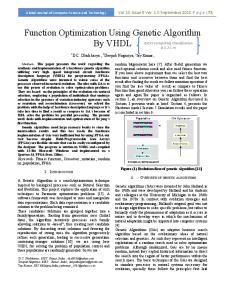
The advantage of SE decomposition is that the time complexity for the morphological operations will be reduced extremely. The time complexity for dilation (erosion) operators is proportional to the number of nonzero element of S. Fig. 1(a-b) shows two examples. The first is to decompose a square SE of size 5×5 into two row vectors of size 1×3 and two column vectors of size 3×1, and the computation time will decrease from 25 to 3+2+3+2=10. The second example is to decompose a diamond SE of diameter 7 into three small SEs, and the time will decrease from 25 to 5+4+4=13.

)†(

†

†

†

†

†

*

Fig. 1. Examples of SE Decomposition: (a) 7×7 Square; (b) 7×7 Diamond; (c) 5×5 Rand

516

Y. Zhang and L. Wu

For parallel pipelined architecture, we decompose the SE using both dilation and union operator. The cost time of the union operator is the maximum of the number of nonzero element of both operands. Fig. 1(c) gives an example, here the subscript (-1,-1) denotes this square matrix should be translated -1 at both x-axis and y-axis. The parallel computation time after decomposition will decrease from 14 to max(3+4,2) = 7.

3 Recursive Model Let SNN denote a SE of size N×N. The first decomposition can be written as S NN = V( N − 2)( N − 2) ⊕ F33PC ∪ RNN

(3)

Here we use the dilation and union model: the V denotes the variable-size matrix of SE, the FPC denotes the fixed-size prime component, and R denotes the residue component. The R can be easily decomposed into union of factors of size 3×3 because the size 3×3 is often used as the elementary structuring component for decomposition in literature. 1 S NN = V( N − 2)( N − 2) ⊕ F33PC ∪ ⎡⎢( R33 )( x1, y1) ∪ ( R332 )( x 2, y 2) ∪ ⎣

∪ ( R33n )

( xn, yn )

⎤ ⎥⎦

(4)

Here n denotes the number of 3-by-3 residual matrix. The subscript (xi, yi) denotes that the Ri should be translated by (xi, yi). Therefore, the iteration continues to V(N-2)(N2) until the size is smaller or equal to 3×3. The flow of the recursive decomposition model is depicted in Fig. 2.

S NN = V( N −2)( N −2) ⊕ F33PC ∪ RNN 1 RNN = ( R33 )

( x1, y1)

∪ ( R332 )

( x 2, y 2)

∪

∪ ( R33nk )

( xnk , ynk )

Fig. 2. Flow of Recursive Decomposition Model

Recursive Structure Element Decomposition

517

Fig. 2 indicates we record 4 variables (Vk, Fk, Rk, and Pk) at each iteration level k, and the decomposition tree can be depicted via those variables. Our task is to develop an effective method to decompose formula (3).

4 Optimization Problem GA simulates the process of natural selection, and is well suited to optimize solutions over large combinatorial spaces [6]. To apply GA in decomposition model, the encoding strategy and the fitness function should be determined first, which are presented in the following. For the encoding strategy, we encoded the variable Fk and straighten it into a onedimensional string of chromosome. For any SE at any iteration, the Fk is a 3-by-3 two-value image, therefore, the chromosome can be written as

ξ

straighten( F ) = f1 f 2 ... f 9

(5)

Here ξ denotes the chromosome and fi denotes the locus. Fig. 3(a) illustrates the numbering scheme for ξ. Two examples are shown in Fig. 3(b-c), and their 1D string of chromosomes are “100101011” and “011001101” respectively. 1

2

3

1

0

0

0

1

1

4

5

6

1

0

1

0

0

1

7

8

9

0

1

1

1

0

1

Fig. 3. (a) Index of gene positions with two examples: (b) “100101011”; (c) “011001101”.

For the fitness function, the prime component F is encoded, therefore, variable matrix of SE V and residual matrix R can be obtained through following formulas V =S – F

(6)

R = S −V ⊕ F

(7)

Then, we can extract two different types of costs. One is serial computation cost JS, and the other is parallel computation cost JP. Note that those variables satisfy the equality of S = V ⊕ F ∪ R , the costs are written as J S = ∑V + ∑ F + ∑ R

(8)

JP = ∑ R

(9)

In this paper, we combine those two costs with a weight factor ω, viz. J = ω JS +(1-ω) JP. For simplicity, ω=0.5.

518

Y. Zhang and L. Wu

5 Migration Fitness Scaling GA GA is efficient and has the ability of jumping out of local minima, but some times it spends excessive time on redundant iteration [7]. To overcome this problem, we proposed a novel migration fitness-scaling GA (MFSGA) which combines the migration model and the fitness scaling strategy. The migration model takes the idea of separately evolving subpopulations and extends it by adding a means of selectively sharing genetic information between them. Migration may occur in a variety of ways. Two parameters associated with the migration algorithm [8] are extremely important: the migration interval and the migration rate. The migration interval is the number of generations between each migration, and the migration rate is the number of individuals selected for migration. For each subpopulation in the distributed GA, migration is accomplished as follows. Every migration interval, the best individuals from one subpopulation replace the worst individuals in its neighbor. Individuals that migrate from one subpopulation to another are copied. They are not removed from the source subpopulation. As with multiple elitist selection, migration represents a tradeoff between exploration of new designs and exploitation of highly fit designs which have already been found. The physical relationship between subpopulations imposed by the topology of the distributed system has an effect on this tradeoff as well. The ring topology used for the proposed migration model ensures local communications between subpopulations. The benefit of this design is that migration occurs locally between adjacent populations on the ring. This yields local exploitation of fit designs, while globally the separate subpopulations are free to explore different types of designs independently [9]. Fitness scaling is the other improvement, which converts the raw fitness scores that are returned by the fitness function to values in a range that is suitable for the selection function [10]. The selection function uses the scaled fitness values to select the particles of the next generation. Then, the selection function assigns a higher probability of selection to particles with higher scaled values. There exist bundles of fitness scaling methods. The most common scaling techniques include traditional linear scaling, rank scaling, power scaling, and top scaling. Among those fitness scaling methods, the power scaling finds a solution nearly the most quickly due to improvement of diversity but it suffers from unstability [11], meanwhile, the rank scaling show stability on different types of tests. Therefore, a new power-rank scaling method was proposed combing both power and rank strategies as follows

fiti = ri k / ∑ i =1 ri k N

(10)

where ri is the rank of ith individual, N is the number of population. Our strategy contains a three-step process. First, all individuals are sorted to obtain the ranks. Second, powers are computed for exponential values k. Third, the scaled values are normalized by dividing the sum of the scaled values over the entire population.

Recursive Structure Element Decomposition

519

6 Experiments The experiments were carried out on the platform of P4 IBM with 3GHz processor and 2GB memory, running under Windows XP operating system. The algorithm was developed via the global optimization toolbox of Matlab 2010b. The SE shown in Fig. 4 is indecomposable by Park’s algorithm [3]. However, a successful decomposition can be found via our algorithm as shown in Fig. 4(a). The serial computation cost is 10 and the parallel computation cost is 1. We run both our proposed improved GA and the CGA in Shih’s method 20 times [4] without using Park’s 13 prime factor as initialization population. Our method all finds the global best result, while three runs of CGA finds a failed result as shown in Fig. 4(b) with serial computation cost of 11 and parallel computation cost of 2. Therefore, the proposed improved GA is more robust than the CGA algorithm of Shih’s algorithm.

(

)⊕

(

⊕

)⊕

⊕

∪

∪ (1,-1)

(-1,-2)

Fig. 4. A typical decomposition tree: (a) A success run; (b) A failed run

=

(

)⊕

(

)⊕

∪

∪ (-2,2)

⊕

∪

∪ (0,-2)

(2,2)

∪ (-1,1)

(0,-1)

Fig. 5. Decomposition tree of Anelli’s SE Fig. 5 shows the decomposition tree of Anelli’s SE. We compared our method with Anelli’s paper [12]. The serial computation cost of our algorithm is 18, and the parallel computation cost of our algorithm is 6. Conversely, the serial and parallel computation costs of Anelli’s method are 22 and 10, respectively. The decomposition tree of Anelli can be seen in Ref. [12]. We use 4 examples of 15-by-15 different shapes including the letter “V”, heart, and umbrella. Tab. 1 lists their original SE shape, the decomposition tree, the serial computation cost, and the parallel computation cost. For the V-shaped SE, the original points are 94, the serial and parallel computation cost after decomposition is only 94 and 13, respectively. For the heart, the points of original SE, JS, and JP are 142, 32, and 8, respectively. For the umbrella, the points of original SE, JS, and JP are 94, 44, and 27, respectively.

520

Y. Zhang and L. Wu Table 1. Three Decomposition Examples (black denotes 0 & white denotes 1) Original SE & its points

Decomposition Tree (

)⊕

∪

)⊕

∪

)⊕

32

8

44

27

(2,1)

∪

)⊕

∪

∪ (-3,0)

(

13

∪ (1,-2)

(-4,4) (

29

(6,6)

∪ (0,-5)

(

JP

∪ (-6,6)

(

JS

(-3,-3)

)⊕

(94) ⊕

∪ (1,1)

(

)⊕

∪

(

)⊕

∪

(

)⊕

(

)⊕

(-1,-5)

(-1,-3)

∪

∪ (-3,3)

(

)⊕

(3,3)

∪ (-2,2)

(142) ⊕

∪

∪ (-1,1)

(

)⊕

∪

∪ (-3,-6)

(

)⊕

∪

(

)⊕

∪

∪ (-4,4)

)⊕

∪ (-6,3)

(-2,-6)

∪ (-5,4)

(

(1,1)

(5,4)

∪ (-2,-4)

(2,4)

∪ (-2,-3)

(

)⊕

∪

∪ (-2,2)

(94) ⊕

∪

(-1,-2)

∪ (1,1)

(-1,1)

7 Conclusions In this paper, a decomposition method for arbitrarily-shaped structuring elements is proposed based on recursive model and migration fitness scaling genetic algorithm. The MFSGA method uses the ring topology of the migration model and the powerrank scaling strategy. Compared to Park’s method [3], Anellie’s method [12], and Shih’s method [4], our method is more robust and have higher rate to find global minima. The future work will focus on applying the proposed MFSGA method to various industrial fields including image classification [13], pattern recognition [14], and weights optimization [15].

Recursive Structure Element Decomposition

521

References 1. Burgeth, B., Bruhn, A., Papenberg, N., Welk, M., Weickert, J.: Mathematical morphology for matrix fields induced by the Loewner ordering in higher dimensions. Signal Processing 87, 277–290 (2007) 2. Park, H., Yoo, J.: Structuring element decomposition for efficient implementation of morphological filters. In: IEE Proceedings of Vision, Image and Signal Processing, vol. 148, pp. 31–35 (2001) 3. Hashimoto, R.F., Barrera, J.: A note on Park and Chin’s algorithm [structuring element decomposition]. IEEE Transactions on Pattern Analysis and Machine Intelligence 24, 139– 144 (2002) 4. Shih, F.Y., Wu, Y.-T.: Decomposition of binary morphological structuring elements based on genetic algorithms. Computer Vision and Image Understanding 99, 291–302 (2005) 5. Zhang, Y., Wu, L.: Stock Market Prediction of S&P 500 via combination of improved BCO Approach and BP Neural Network. Expert Systems with Applications 36, 8849–8854 (2009) 6. Zhang, Y., Yan, J., Wei, G., Wu, L.: Find multi-objective paths in stochastic networks via chaotic immune PSO. Expert Systems with Applications 37, 1911–1919 (2010) 7. Rausch, T., Thomas, A., Camp, N.J., Cannon-Albright, L.A., Facelli, J.C.: A parallel genetic algorithm to discover patterns in genetic markers that indicate predisposition to multifactorial disease. Computers in Biology and Medicine 38, 826–836 (2008) 8. Rom, W.O., Slotnick, S.A.: Order acceptance using genetic algorithms. Computers & Operations Research 36, 1758–1767 (2009) 9. Omara, F.A., Arafa, M.M.: Genetic algorithms for task scheduling problem. Journal of Parallel and Distributed Computing 70, 13–22 (2010) 10. Tkaczyk, E.R., Mauring, K., Tkaczyk, A.H., Krasnenko, V., Ye, J.Y., Baker Jr, J.R., Norris, T.B.: Control of the blue fluorescent protein with advanced evolutionary pulse shaping. Biochemical and Biophysical Research Communications 376, 733–737 (2008) 11. Korsunsky, A.M., Constantinescu, A.: Work of indentation approach to the analysis of hardness and modulus of thin coatings. Materials Science and Engineering: A 423, 28–35 (2006) 12. Anelli, G., Broggi, A., Destri, G.: Decomposition of arbitrarily shaped binary morphological structuring elements using genetic algorithms. IEEE Transactions on Pattern Analysis and Machine Intelligence 20, 217–224 (1998) 13. Zhang, Y., Wang, S., Wu, L.: A Novel Method for Magnetic Resonance Brain Image Classification based on Adaptive Chaotic PSO. Progress in Electromagnetics Research 109, 325–343 (2010) 14. Zhang, Y., Wu, L.: Pattern recognition via PCNN and Tsallis entropy. Sensors 8, 7518– 7529 (2008) 15. Zhang, Y., Wu, L.: Weights optimization of neural network via improved BCO approach. Progress in Electromagnetics Research 83, 185–198 (2008)