Pricing and Hedging European Options on Futures Spreads Using the Bachelier Spread Option Model by Matthew P. Schaefer
Suggested citation format: Schaefer, M. P. 2002. “Pricing and Hedging European Options on Futures Spreads Using the Bachelier Spread Option Model.” Proceedings of the NCR-134 Conference on Applied Commodity Price Analysis, Forecasting, and Market Risk Management. St. Louis, MO. [http://www.farmdoc.uiuc.edu/nccc134].
Pricing and Hedging European Options On Futures Spreads Using the Bachelier Spread Option Model
Matthew P. Schaefer*
Paper Presented at the NCR-134 Conference on Applied Commodity Price Analysis, Forecasting, and Market Risk Management St. Louis, Missouri, April 22-23, 2002
Copyright 2002 by Matthew P. Schaefer. All rights reserved. Readers may make verbatim copies of this document for non-commercial purposes by any means, provided that this copyright notice appears on all such copies.
* Matthew P. Schaefer is a research manager at the New York Mercantile Exchange. The author would like to thank Geoffrey Poitras for reviewing an earlier version of this paper.
Pricing and Hedging European Options On Futures Spreads Using the Bachelier Spread Option Model The Bachelier model for pricing options on futures spreads (OFS) assumes changes in the underlying futures prices and spread follow unrestricted arithmetic Brownian motion (UABM). The assumption of UABM allows for a convenient analytic solution for the price of an OFS. The same is not possible under the more traditional assumption of geometric Brownian motion (GBM). Given the additional complexity of methods for pricing and hedging OFS using GBM such as Monte Carlo simulation and binomial trees, it is worth investigating how results from the Bachelier model compare to these other methods. The Bachelier model is presented and then extended to price an OFS with three underlying commodities. Hedge parameters for both models are provided. Results indicate that for OFS with sufficiently low volatility, differences between the Bachelier model and methods assuming GBM are quite small. Key Words: spread options, crack spread, soybean crush spread. Introduction Options on futures spreads (OFS) are now traded derivatives in over-the-counter agriculture and energy markets, and also at the New York Mercantile Exchange. As recognized by Shimko and Poitras, OFS have been considered by at least three futures exchanges: the New York Mercantile Exchange (NYMEX) currently lists 1:1 options on crack (fuel) futures spreads and has proposed a 3:2:1 crack spread option and energy calendar spread options, the New York Board of Trade (NYBOT) proposed a cotton calendar spread option, and the Chicago Board of Trade (CBOT) has considered trading options on the soybean crush spread. In addition, there are credit spreads such as the TED spread between the Eurodollar and Treasury bill rates, and there are spreads based on variations in location and grade. Despite their growing popularity and effectiveness for managing certain types of risk such as commodity transformation, short-term storage and basis risk, little publicly available research has focused on pricing and hedging these derivatives, especially for spreads involving three underlying commodities. Motivating this paper is the fact that a closed form solution for pricing OFS under the assumption that the underlying legs follow correlated geometric Brownian motions (GBM) does not exist. Instead analytic approximations or numerical methods such as Monte Carlo simulation and binomial trees must be used. Poitras provides an analytic pricing solution based on the work of the French mathematician Bachelier based on the assumption that the underlying spread follows unrestricted arithmetic Brownian motion (UABM). The Bachelier model is easy to implement and hedge parameters are easily derived. Provided the underlying spread is normally distributed the Bachelier model is a good starting point for pricing OFS. While UABM does have certain theoretical disadvantages that are discussed later, it is worth investigating its usefulness for pricing OFS relative to other methods that assume the spread is the difference between two correlated log-normally distributed variables given that they are more complicated to implement and hedge and in some cases more computer intensive to implement. In what follows the Bachelier model for call and put OFS are presented. Premiums from the model are then compared with those from a Jarrow-Rudd analytic approximation based on 1
the Bachelier model, and Monte Carlo simulation and binomial methods each under the assumption of GBM. Hedge parameters for the Bachelier model appear in the appendix. In addition, the Bachelier model is extended to price OFS when three underlying commodities are involved. Hedge parameters for the three commodity Bachelier model also appear in the appendix. The results indicate that for OFS with sufficiently low volatility the Bachelier model and other approaches generate nearly identical results. This is good news for practitioners that need to price OFS with sufficiently low volatility and time to maturity. However, as time to maturity and volatility increase so do differences between the Bachelier model and the other approaches. Different Pricing Methods Below is a brief review of the different methods used in this study to price OFS. Bachelier Model Poitras provides the closed form Bachelier model for pricing European OFS spreads. The model assumes the underlying prices follow UABM. This implies that the distribution of the underlying prices (and spread) is normal and that the spread is treated as a single random variable. The partial differential equation that satisfies the riskless hedge portfolio problem has a single delta hedge ratio and gamma, whereas in general there will be two delta hedge ratios, one for each leg of the spread. Since UABM allows for negative sample paths, probability is assigned to negative paths and call options will be priced higher than they otherwise would be under restricted arithmetic Brownian motion. Spread option pricing formulas that assume restricted arithmetic Brownian motion (with an absorbing barrier at zero) can be derived but are complicated and only differ from unrestricted prices when there is a significant probability of the price process reaching zero (Heaney and Poitras). Furthermore, negative sample paths are generally not an issue for commodity prices and are easily identifiable as a potential problem (Poitras). While the validity of the normality assumption should be dealt with on a spread to spread basis, Schaefer shows that premiums from the Bachelier model are nearly identical to premiums from Monte Carlo simulation assuming GBM when the spread volatility and time to maturity are sufficiently low. Jarrow-Rudd Approximation to “True” Solution Shimko presents an analytic approximation based on the Wilcox model that approximates a single integral solution for the price of an option on a spread with stochastic convenience yield where the underlying prices are assumed to follow GBM. Shimko applies the Jarrow-Rudd technique using the Wilcox model to approximate the true solution. This paper does not explore the evaluation of the integral solution and instead focuses on the approximation using the Bachelier model as the approximating model assuming non-stochastic convenience yield. Shimko shows that when the spread volatility (in annualized dollar terms) is below $3.74 ($7.48) for a 12 month (1 month) option one can expect the pricing error to be bounded by $0.025, or less than 1/32. However, as this study highlights, the approximation diverges from the “true” GBM solution over relevant ranges as volatility and time to maturity increase, oftentimes before its usefulness over the Bachelier model is relevant. Nevertheless this method can be useful for pricing long dated spread options with sufficiently low volatility, and can also be extended to the three commodity case. Hedge parameters for this model are difficult due to the inclusion of skewness and kurtosis.
2
Monte Carlo Simulation The Monte Carlo simulation approach is a discrete numerical approximation to the true analytic solution, in this case where the underlying prices follow GBM (see Hull for a review). At the limit this approach converges to the true solution. An acceptable level of convergence is usually reached after a large number of simulations even though variance reduction techniques can be implemented to reduce the number of simulations. Because hedge parameters are obtained by re-pricing the derivative for a small change in the relative input variable this process is inefficient for constantly updating entire options’ series even by today’s PC processor speeds. The Monte Carlo method is used here as a reference for results from the Bachelier model and the analytic approximation. Binomial Trees The binomial tree method is also a discrete approximation to the true analytic solution that can be implemented under the assumption that the underlying prices follow GBM (see Hull for a review). This method also converges to the GBM solution at the limit, but the speed of convergence requires less iterations than the Monte Carlo technique. Of the three methods that assume the underlying prices follow GBM compared in this paper, binomial trees are superior in both computational speed and accuracy, but do come with added complexity, more so for spreads involving three commodities. The methodology for the two commodity case is outlined by Hull. The binomial method is used here as a second reference for results from the Bachelier model and the analytic approximation. Using the European Bachelier Model To Price an OFS (Two Commodity Case) Shimko derives a single-integral solution for the value of a call spread option with stochastic convenience yield based on the assumption that the underlying assets follow correlated geometric Brownian motions. Using the Wilcox model Shimko derives an analytic approximation to this solution based on the Jarrow and Rudd technique. This technique involves approximating the true distribution of the underlying spread by a more tractable approximating distribution using a generalized Edgeworth series expansion. The approximating formula uses the known pricing solution given the approximating distribution and adjusts it based on the skewnesss and kurtosis of the true distribution relative to the approximating distribution. Here the Bachelier model is used as the base model in the analytic approximation. The derivation of the Bachelier model and the analytic approximation with constant convenience yield are presented below. The Approximating Distribution Following the techniques used by Jarrow and Rudd and Shimko for computing the central moments of the underlying spread, the Bachelier model for an OFS under the assumption of normality is presented first. The normal distribution is then used as the approximating distribution for the true GBM solution of the spread value. This leads to an analytic approximation based on the Bachelier model. Based on the standard assumptions of perfect markets and continuous trading, the absence of arbitrage solution to the Bachelier call option pricing result is as follows: (1)
C ( A) = e − rt
*
(
µ 2 d N [d ] + n[d ] µ 2
) 3
where d=
F1 − F2 − X
µ2
µ 2 = σ s2 t * = (σ 12 + σ 22 − 2σ 12 ) t * where C ( A) is the price of the Bachelier futures spread call option, F1 is the price of the underlying long position, F2 is the price of the underlying short position, t * is time to expiration as a fraction of a year ((T − t ) / 365) where T is the option’s expiration date and t is the current date, r is the risk free interest rate, X is the strike price, N[d] and n[d] are the cumulative normal probability density function and normal density function, respectively, evaluated at d, µ 2 is the second central moment of the future difference between F1 and F2 (defined below), where σ s is the annualized standard deviation of daily changes in the value of the spread, and σ 12 is the covariance of daily changes in the value of the spread. Under the same assumptions the Bachelier put option pricing result is as follows: (2)
P( A) = e − rt
*
(
µ 2 d ( N [d ] − 1) + n[d ] µ 2
)
where P( A) is the price of the Bachelier futures spread put option, and all other variables have been previously defined. The mean of the approximating distribution is F1 − F2 and the variance is σ 2 t * . The skewness is zero, and the adjusted kurtosis is zero. The True Distribution Define two correlated geometric Brownian motion processes for futures contracts: dF1 = σ 1 F1 dW1 (3)
dF2 = σ 2 F2 dW 2 dW1 dW 2 = p dt
The next step is to compute the central moments of the future difference between F1 and F2 given the true distribution. Let Z be the difference between F1 and F2 . Then the mean of Z is m = m10 − m 01 , where the expectation m kj is defined as follows: (4)
(
) (
) ({ (
) (
)
The central moments up to order four are shown below: (5)
} )
mkj ≡ E F1k F2j = F1k F2j exp k .5 (k − 1)σ 12 + j .5( j − 1)σ 22 + jkρσ 1σ 2 t *
µ 2 = (m 20 − 2m11 + m 02 ) − m 2
µ 3 = (m30 − 3m 21 + 3m12 − m 03 ) − 3m(m 20 − 2m11 + m 02 ) + 2m 3 4
µ 4 = (m40 − 4m31 + 6m22 − 4m13 + m04 ) − 4m(m30 − 3m21 + 3m12 − m03 ) + 6m 2 (m20 − 2m11 + m02 ) − 3m 4
The skewness and adjusted kurtosis are determined to be (6)
κ 3 = µ3 κ 4 = µ 4 − 3µ 22
Here the first and second moments of the approximating and true distributions are matched. Then call option formula (1) is used as the approximating formula and the expression for the approximate option price is (7)
C (F ) = e
d=
− rt *
(
)
2 κ d µ 2 d N [d ] + n[d ] µ 2 − 3 + κ 4 d µ3 22 − 1 6µ 2 24 µ 2
F1 − F2 − X
µ2
The expression for the put option based on formula (2): (8)
(
)
* κ d κ d 2 µ 2 − 1 P(F ) = e − rt µ 2 d ( N [d ] − 1) + n[d ] µ 2 − 3 + 4 6µ 2 24 µ 23 2
To apply the Bachelier model, use the Black implied volatility for σ 1 and σ 2 and compute ρ (see appendix for deriving implied correlations). Calculate the moment µ 2 and calculate call and put prices from (1) and (2). To apply the analytic approximation, calculate the moments µ 2 through µ 4 , κ 3 and κ 4 , and calculate call and put prices from (7) and (8). Poitras specifies volatility in the Bachelier model using σ s , which is a dollar figure. Here the model has been specified in terms of µ 2 , which relies on percent volatility. This approach should be more convenient to practitioners because it allows for the use of standard methods of calculating volatility developed for regular options. It also allows for the model to be directly compared to most other alternative methods for pricing OFS. Using the European Bachelier Model To Price an OFS (Three Commodity Case) The potential for an OFS involving three underlying commodities is also of interest. Commodity transformation spreads in oil refining and the soybean complex have been considered by major exchanges. Consider the 3:2:1 crack spread, which is two parts unleaded gasoline plus one part heating oil minus three parts crude oil. It is possible to synthetically trade the 3:2:1 crack spread by using one NYMEX 1:1 heating oil crack spread and two NYMEX 1:1 gasoline crack spreads as “building blocks”.1 However, this scheme is more expensive for two reasons. First it has additional “optionality” because each option can be exercised independently of the others. 1
NYMEX 1:1 crack spread options have American exercise style. 5
Second the sum of the volatility for each “block” is more than the volatility of the single 3:2:1 underlying spread. Related spreads include the 1:1:1 soybean crush spread which is one part bean oil plus one part soybean meal minus one part soybeans, and the 2:1:1 cattle crush spread which is one part feeder cattle plus one part corn minus two parts live cattle. The Approximating Distribution Due to the linearity properties of the normal distribution extending the Bachelier model and the Jarrow-Rudd approximation to price an OFS consisting of three underlying commodities is straightforward. Below pricing formulas for the Bachelier model and the analytic approximation are given for the case of a spread in the form (F1 + F2 − F3 ) such the 3:2:1 crack spread and the 1:1:1 soybean crush spread (i.e. it would not be appropriate for the cattle crush spread which has the form (F1 − F2 − F3 ) ). To begin assume that the individual price processes each follow UABM where the appropriate weights are assumed to have been pre-multiplied by the price. The price spread will follow the diffusion: (9)
d (F1 + F2 − F3 ) = σ s dWs
where the variance of the joint process is specified as
σ s2 = σ 12 + σ 22 + σ 32 + 2σ 12 − 2σ 13 − 2σ 23 Here the spread is treated as a single random variable that is normally distributed. The partial differential equation (PDE) associated with the risk hedge portfolio problem for a futures price following UABM can then be invoked which gives (10)
∂C 1 ∂ 2C + σ s2 = rC ∂t 2 ∂ (F1 + F2 − F3 )
Because the spread is treated as a single random variable this PDE involves only one delta hedge ratio and one gamma. The Bachelier call option formula that satisfies this PDE is given by (11)
C ( A) = e − rt
*
(
µ 2 d N [d ] + n[d ] µ 2
)
where d=
F1 + F2 − F3 − X
µ2
µ 2 = σ s2 t * = (σ 12 + σ 22 + σ 32 + 2σ 12 − 2σ 13 − 2σ 23 ) t * Under the same assumptions the put option pricing result is as follows:
6
(12)
P( A) = e − rt
*
(
µ 2 d ( N [d ] − 1) + n[d ] µ 2
)
where P( A) is the price of the Bachelier futures spread put option. Substitution of the derivatives theta [formulas A.30 (call) and A.31 (put)] and gamma (A.21) into (10) proves (11) and (12). The True Distribution Define three correlated geometric Brownian motion processes for futures contracts:
(13)
dF1 = σ 1 F1 dW1
dW1 dW 2 = p12 dt
dF2 = σ 2 F2 dW 2
dW1 dW3 = p13 dt
dF3 = σ 3 F3 dW3
dW 2 dW3 = p 23 dt
Next compute the central moments of the future difference between F1 + F2 and F3 given the true distribution. Let Z be the difference between F1 + F2 and F3 . Then the mean of Z is m = m100 + m 010 − m 001 , where the expectation m kji is defined as follows: (14)
(
) (
) (
)
k .5 (k − 1)σ 12 + j .5( j − 1)σ 22 + i .5(i − 1)σ 32 + kjρ12σ 1σ 2 * mkji ≡ E F F2 F = F F2 F exp t + kiρ σ σ + jiρ σ σ 13 1 3 23 2 3
(
k 1
j
i 3
) (
k 1
j
i 3
)
The central moments up to order four (see Kendall and Stuart 1977, p. 73) are below: (15)
µ 2′ = (m 200 + m 020 + m 002 + 2m110 − 2m101 − 2m 011 ) µ 3′ = (m300 + m 030 − m 003 + 3m 210 − 3m 201 + 3m120 − 3m 021 + 3m102 + 3m 012 − 6m111 ) m
+m
+m
+ 4m
− 4m
+ 4m
− 4m
040 004 310 301 130 031 µ 4′ = 400 + 6m 220 + 6m 022 + 6m 202 − 12m 211 − 12m121 + 12m112
and
µ 2 = µ 2′ − m 2 µ 3 = µ 3′ − 3mµ 2′ + 2m 3 µ 4 = µ 4′ − 4mµ 3′ + 6m 2 µ 2′ − 3m 4 The skewness and adjusted kurtosis are determined to be (16)
κ 3 = µ3 κ 4 = µ 4 − 3µ 22
7
− 4m 013 − 4m103
The call option formula (11) is used as the approximating formula and the expression for the approximate option price is (17)
(
)
* κ d κ d 2 µ 2 − 1 C (F ) = e − rt µ 2 d N [d ] + n[d ] µ 2 − 3 + 4 6µ 2 24 µ 23 2
d=
F1 + F2 − F3 − X
µ2
The approximating formula for the put option based on (12) is (18)
(
)
* κ d κ d 2 µ 2 − 1 P(F ) = e − rt µ 2 d (N [d ] − 1) + n[d ] µ 2 − 3 + 4 6µ 2 24µ 23 2
To apply the Bachelier model, use the Black implied volatility for σ 1 , σ 2 , and σ 3 and compute each ρ . Calculate the moment µ 2 and calculate call and put prices from (11) and (12). To apply the analytic approximation, calculate the moments µ 2 through µ 4 , κ 3 and κ 4 , and calculate call and put prices from (17) and (18). Accuracy The analytic approximation can be checked using Monte Carlo simulation. Three correlated samples ε 1 , ε 2 and ε 3 from standard normal distributions are required. First obtain independent samples x1 , x 2 and x 3 from a univariate standardized normal distribution. The required samples ε 1 , ε 2 and ε 3 are then calculated as follows:
ε 1 = x1 (19)
ε 2 = x1 ρ 12 + x 2 1 − ρ 122 ε 3 = x1 ρ 13 + x 2
ρ 23 − ρ 13 ρ 12 1 − ρ 122
+ x3
ρ −ρ ρ 13 12 1 − ρ 132 − 23 1 − ρ 122
2
Sensitivity Analysis The first part of this section presents call option premiums using the two commodity European Bachelier model. The premiums are compared to those using the Jarrow-Rudd analytic approximation, and Monte Carlo simulation and binomial tree methods each under the assumption that the spread is the difference between to correlated log-normally distributed random variables. Options with different volatilities and times to maturity are evaluated. Table 1 presents results for options one month, three months, and one year to expiration.
The second part of this section presents call option premiums using the three commodity European Bachelier model for a spread in the form (F1 + F2 − F3 ) . The premiums are compared to those using the Jarrow-Rudd analytic approximation and Monte Carlo simulation under the 8
assumption that the underlying prices follow GBM. Options with different volatilities and times to maturity are evaluated. Table 2 presents results for options one month, three months, and one year to expiration. The number of Monte Carlo simulations used was 200,000 for each option premium with time step equal to time to maturity. No variance reduction procedures were used. One hundred iterations were used for the binomial method. The Bachelier model, analytic approximation and Monte Carlo simulations were conducted in VBA. Results from the binomial method were generated using Fintools® software. Two Commodity OFS One Month Options Based on the results in Table 1 the Bachelier model and the analytic approximation are very accurate relative to the Monte Carlo and binomial methods. Differences are less than a penny for OFS for “low” and “medium” range volatility. For OFS with “high” volatility, the Bachelier model is within 1 to 2 cents of the Monte Carlo and binomial methods and the analytic approximation is generally within a cent.
Three Month Options For OFS three months to expiration differences between the Bachelier model and the analytic approximation are within a penny of the Monte Carlo and binomial methods for low range volatility spreads. For medium range volatilities the Bachelier model differences increase to about 3 pennies relative to the Monte Carlo and binomial methods, while the analytic approximation remains consistent. This is a good example of the when the analytic approximation is still relatively consistent with the GBM solution while the Bachelier model is not. This will generally be true for OFS with low to medium range volatility with two or more months to expiration (see Figure 1). However, the error of the approximation should always be a concern of the practitioner. For OFS in the high volatility range the Bachelier model differences relative to the Monte Carlo and binomial methods grow to about 12 cents. We also start to see the analytic approximation start to diverge (see Figure 3)2. One Year Options OFS in the low volatility range are still consistent across each method. Differences are generally less than a penny. In the medium range case differences between the Bachelier model and the Monte Carlo and binomial methods are quite significant growing to as much as 20 cents. The analytic approximation is also significantly different, nearly 13 cents under the numerical methods. As expected, the difference grows between the Bachelier model and analytic approximation relative to the numerical methods as volatility increases. The Bachelier model premiums are around 1 dollar more and the analytic approximation is actually negative in the high volatility case (see Figure 3). Three Commodity OFS Results of the sensitivity analysis conducted for the three commodity Bachelier model are presented in Table 2. Results are consistent with results for the two commodity case. In general, the Bachelier model is consistent with the GBM solution (in this case approximated by just the 2
20,000 Monte Carlo simulations were used to create Figure 3 in order to illustrate the binomial method. 9
Monte Carlo method) for OFS in the low volatility range for each time to maturity tested. Differences increase as volatility and time to expiration increase. Likewise, the analytic approximation is consistent with the Monte Carlo method for OFS with relatively low volatility but begins to significantly diverge at approximately two and a half months to maturity for the high volatility case (see Figure 4). As for the two commodity case, there are ranges over which the analytic approximation will be more accurate than the Bachelier model relative to the GBM solution given different volatilities and times to maturity. However, the error of the approximation must be monitored (see Figure 2). Conclusion Options on futures spreads are currently traded in over the counter agriculture and energy derivatives markets and also at the New York Mercantile Exchange. Additional contracts have been proposed by leading exchanges. Despite their growing popularity and effectiveness for managing certain types of risk such as commodity transformation, short-term storage and basis risk, little publicly available research has focused on pricing and hedging these derivatives, especially for spreads involving three underlying commodities such as the crack (fuel) spread and the soybean crush spread. While methods for pricing an OFS exist there is little information on how different methods compare.
Here the Bachelier model is presented and hedge parameters are provided. The closed form Bachelier model assumes the underlying spread follows unrestricted arithmetic Brownian motion. An analytic approximation for the price of an OFS under the assumption that the underlying prices follow correlated geometric Brownian motions is also presented. The two methods are then extended to price an OFS with three underlying commodities. Next the Bachelier model is compared to Monte Carlo simulation and binomial tree methods that assume the underlying prices follow correlated geometric Brownian motions for spreads with two and three underlying commodities. Results from the sensitivity analysis indicate that for OFS with two and three underlying commodities that have sufficiently low volatility, the Bachelier model and the analytic approximation are very consistent with Monte Carlo and binomial methods. However, as time to maturity and volatility increase so do differences between the Bachelier model and the analytic approximation relative to the numerical methods. Given that alternative methods for pricing OFS under the assumption of geometric Brownian motion and restricted arithmetic Brownian motion are more complicated, the Bachlier model should be of particular interest to practitioners who place a premium on ease of implementation, tractable hedge parameters and computational speed in addition to pricing accuracy.
10
Appendix Hedge Parameters For the Bachelier Model (Two Commodity Case) Poitras gives solutions for the delta, gamma and theta for the Bachelier call spread option. Provided here are the delta, gamma, vega, theta and rho for the Bachelier call and put option.
Delta Delta for the spread (F1 − F2 ) and for the individual legs from the Bachelier futures spread call option are as follows: (A.1)
* ∂C ( A) ∂C ( A) = = e − rt N [d ] ∂ (F1 − F2 ) ∂F1
(A.2)
* ∂C ( A) = −e −rt N [d ] ∂F2
Delta for the spread and individual legs from the Bachelier futures spread put option are as follows: (A.3)
* ∂P( A) ∂P( A) = = e −rt ( N [d ] − 1) ∂ (F1 − F2 ) ∂F1
(A.4)
* ∂P( A) = −e − rt ( N [d ] − 1) ∂F2
Delta can be interpreted the same as for the Black model. Gamma Gamma for the spread and the individual legs from the Bachelier futures spread call and put option is as follows: e − rt n[d ] *
(A.5)
Γ=
µ2
Vega Vega for the spread, from the Bachelier futures spread call and put option, is as follows: (A.6)
* ∂C ( A) ∂P( A) = = e − rt n[d ] t * ∂σ s ∂σ s
Vega with respect to σ 1 for a call and put option is as follows: *
(A.7)
(
* − rt µ 2,1 − µ 2, 2 ρ ∂C ( A) ∂P( A) e n[d ] t = = ∂σ 1 ∂σ 1 µ2
where the moments µ 2,1 and µ 2, 2 are as follows:
11
)
(A.8)
( ) ≡ E (F ) = F
(( ) ) exp( j (.5( j − 1)σ ) t )
mk ,1 ≡ E F1k = F1k exp k .5(k − 1)σ 12 t * m j,2
j
2
2
j
2 2
*
µ 2,1 = m 2,1 − m12,1 µ 2, 2 = m 2, 2 − m12, 2 Vega with respect to σ 2 for a call and put option is as follows:
(
* − rt µ 2, 2 − µ 2,1 ρ ∂C ( A) ∂P( A) e n[d ] t = = ∂σ 2 ∂σ 2 µ2 *
(A.9)
)
Vega can be interpreted as follows: for a one dollar increase in the value of σ s , σ 1 , or σ 2 , respectively, the value of the option will increase by vega. The change in the value of the option premium given a one percent change in correlation can be computed as follows: (A.10)
e ∂C ( A) ∂P( A) = =− ∂ρ ∂ρ
− rt *
n[d ] µ 2,1 µ 2, 2
µ2
÷ 100
Theta From the Bachelier spread call option model it can be shown that theta per annum is as follows: (A.11)
(
)
* ∂C ( A) 1 − rt * n[d ] 2rt − 1 µ 2 e = − − 2r (F1 − F2 − X )N [d ] * * 2 t ∂t
For a Bachelier spread put option it can be shown that (A.12)
(
)
* ∂P( A) 1 − rt * n[d ] 2rt − 1 µ 2 e = − − 2r (F1 − F2 − X )(N [d ] − 1) * * 2 t ∂t
When time is measured in days, theta per day = [theta per annum/365]. Rho From the Bachelier spread call option model it can be shown that rho is as follows: (A.13)
∂C ( A) = C ( A) t * ÷ 100 ∂r
For a Bachelier spread put option the rho is as follows: (A.14)
∂P( A) = P( A) t * ÷ 100 ∂r
Implied Correlation The implied correlation of the spread can be found using the Newton-Raphson algorithm. To start the search algorithm first find the initial guess of the spread variance based on an initial guess for the correlation: (A.15)
σ s2,i = µ 2,1 + µ 2, 2 − 2 µ 2,1 µ 2, 2 ρ i 12
where σ s ,i is the initial guess for the spread variance, the moments µ 2,1 and µ 2, 2 are computed using implied volatility σ 1 and σ 2 from the Black model, and ρ i is the initial guess for implied correlation. Next find the second guess for ρ : (A.16)
MP − B ρ i
Λ ρi
ρ i +1 = σ s2,i +
− (µ 2,1 ρ i + µ 2, 2 ρ i ) − 2 µ 2,1 ρ i µ 2, 2 ρ i
where MP is the market price of the option, B ρ i is the Bachelier premium conditional on ρ i and Λ ρ i the option’s vega conditional on ρ i . Continue the process until MP − B ρ i < ε where
ε is a specified degree of accuracy. Hedge Parameters For the Bachelier Model (Three Commodity Case)
Delta Delta for the spread (F1 + F2 − F3 ) and for the individual legs from the Bachelier futures spread call option are as follows: (A.17)
* ∂C ( A) ∂C ( A) ∂C ( A) = = = e − rt N [d ] ∂ (F1 + F2 − F3 ) ∂F1 ∂F2
(A.18)
* ∂C ( A) = −e −rt N [d ] ∂F3
Delta for the spread and individual legs from the Bachelier futures spread put option are as follows: (A.19)
* ∂P( A) ∂P( A) ∂P( A) = = = e − rt (N [d ] − 1) ∂ (F1 + F2 − F3 ) ∂F1 ∂F2
(A.20)
* ∂P( A) = −e − rt (N [d ] − 1) ∂F3
Gamma Gamma for the spread and the individual legs from the Bachelier futures spread call and put option is as follows: e − rt n[d ] *
(A.21)
Γ=
µ2
Vega Vega for the spread from the Bachelier futures spread call and put option is as follows: (A.22)
* ∂C ( A) ∂P( A) = = e − rt n[d ] t * ∂σ s ∂σ s
Vega with respect to σ 1 for the call and put option is as follows:
13
* − rt ∂C ( A) ∂P( A) e n[d ] t = = ∂σ 1 ∂σ 1 *
(A.23)
(
µ 2,1 + µ 2, 2 ρ12 − µ 2,3 ρ13
)
µ2
where the moments µ 2,1 , µ 2, 2 , and µ 2,3 are as follows: (A.24)
( ) (( ) ) ≡ E (F ) = F exp( j (.5( j − 1)σ ) t ) ≡ E (F ) = F exp(i (.5(i − 1)σ ) t )
mk ,1 ≡ E F1k = F1k exp k .5(k − 1)σ 12 t * m j ,2 mi ,3
j
j
2
i 3
2 2
2
i 3
2 3
*
*
µ 2,1 = m 2,1 − m12,1 µ 2, 2 = m 2, 2 − m12, 2 µ 2,3 = m2,3 − m12,3 Vega with respect to σ 2 for the call and put option is as follows: * − rt ∂C ( A) ∂P( A) e n[d ] t = = ∂σ 2 ∂σ 2 *
(A.25)
(
µ 2, 2 + µ 2,1 ρ12 − µ 2,3 ρ 23
)
µ2
Vega with respect to σ 3 for the call and put option is as follows: * − rt ∂C ( A) ∂P( A) e n[d ] t = = ∂σ 3 ∂σ 3 *
(A.26)
(
µ 2,3 − µ 2,1 ρ13 − µ 2, 2 ρ 23
)
µ2
The change in the value of the option premium given a one percent change in correlation can be computed as follows: (A.27)
− rt ∂C ( A) ∂P( A) e n[d ] µ 2,1 µ 2, 2 = = ÷ 100 ∂ρ12 ∂ρ12 µ2 − rt *
(A.28)
e ∂C ( A) ∂P( A) = =− ∂ρ13 ∂ρ13
− rt *
(A.29)
e ∂C ( A) ∂P( A) = =− ∂ρ 23 ∂ρ 23
*
n[d ] µ 2,1 µ 2,3
µ2 n[d ] µ 2, 2 µ 2,3
µ2
÷ 100
÷ 100
Theta From the Bachelier spread call option model it can be shown that theta per annum is as follows: (A.30)
(
)
* ∂C ( A) 1 − rt * n[d ] 2rt − 1 µ 2 = − − 2r (F1 + F2 − F3 − X )N [d ] e * * 2 ∂t t
For a Bachelier spread put option it can be shown that
14
(A.31)
(
)
* ∂P( A) 1 − rt * n[d ] 2rt − 1 µ 2 ( ) ( ) = − − + − − − e 2 r F F F X N [ d ] 1 1 2 3 * 2 ∂t * t
When time is measured in days, theta per day = [theta per annum/365]. Rho From the Bachelier spread call option model it can be shown that rho is as follows: (A.32)
∂C ( A) = C ( A) t * ÷ 100 ∂r
For a Bachelier spread put option the rho is as follows: (A.33)
∂P( A) = P( A) t * ÷ 100 ∂r
Implied Correlation The implied correlation for the three commodity case is complicated by the need for three unknown correlations. If two correlations can be implied from 1:1 option premiums (as is the case for the 3:2:1 crack spread) then the third implied correlation can be derived using the Newton-Rhapson algorithm applied to the three commodity case.
15
Table 1 Theoretical Prices of European Futures Spread Options (2 Commodity) Using Bachelier, Shimko, Monte Carlo and Binomial Tree Methods (r = 4%, F1 = $25, F2 = $25, Strike Price = $0, Simulations = 200,000, Iterations = 100) Calls Option Parameters Spread Bachelier Shimko MC Binomial Value -.50 0.03910 0.03923 0.03909 0.03887 σ1 = 15% -.30 0.07996 0.07994 0.08062 0.07984 σ2 = 15% -.10 0.14731 0.14715 0.14789 0.14726 ρ = 90% t* = 1/12 0 0.19267 0.19249 0.19270 0.19263 .10 0.24622 0.24606 0.24587 0.24618 .30 0.37706 0.37704 0.37720 0.37694 .50 0.53517 0.53533 0.53404 0.53496 -.50 0.37259 0.36707 0.36712 0.36790 σ1 = 45% -.30 0.44842 0.44327 0.44459 0.44396 σ2 = 45% -.10 0.53484 0.52990 0.53305 0.53052 ρ = 90% t* = 1/12 0 0.58213 0.57722 0.57904 0.57782 .10 0.63218 0.62726 0.63436 0.62789 .30 0.74058 0.73550 0.73836 0.73619 .50 0.85995 0.85453 0.85737 0.85537 -.50 0.76552 0.73950 0.74206 0.74343 σ1 = 75% -.30 0.84805 0.82297 0.82875 0.82638 σ2 = 75% -.10 0.93712 0.91257 0.91290 0.91571 ρ = 90% t* = 1/12 0 0.98414 0.95970 0.96461 0.96278 .10 1.03285 1.00840 1.01153 1.01153 .30 1.13533 1.11054 1.11563 1.11396 .50 1.24459 1.21904 1.22646 1.22297 -.50 0.14467 0.14372 0.14536 0.14376 σ1 = 15% -.30 0.20647 0.20554 0.20769 0.20571 σ2 = 15% -.10 0.28560 0.28468 0.28547 0.28493 ρ = 90% t* = 3/12 0 0.33208 0.33117 0.33148 0.33142 .10 0.38328 0.38237 0.38247 0.38262 .30 0.49974 0.49883 0.49925 0.49900 .50 0.63413 0.63322 0.63293 0.63325 -.50 0.80026 0.77108 0.77446 0.77558 σ1 = 45% -.30 0.88255 0.85436 0.85916 0.85833 σ2 = 45% -.10 0.97110 0.94348 0.95103 0.94716 ρ = 90% t* = 3/12 0 1.01777 0.99026 0.99682 0.99387 .10 1.06604 1.03853 1.05302 1.04220 .30 1.16744 1.13958 1.14658 1.14353 .50 1.27533 1.24668 1.25492 1.25119 -.50 1.55301 1.38849 1.43473 1.43578 σ1 = 75% -.30 1.63699 1.47503 1.52152 1.52080 σ2 = 75% -.10 1.72491 1.56457 1.60479 1.60949 ρ = 90% t* = 3/12 0 1.77037 1.61048 1.65889 1.65517 .10 1.81684 1.65714 1.69988 1.70189 .30 1.91281 1.75277 1.80050 1.79805 .50 2.01288 1.85150 1.90304 1.89803 -.50 0.44439 0.43622 0.44175 0.43740 σ1 = 15% -.30 0.51980 0.51211 0.51723 0.51307 σ2 = 15% -.10 0.60413 0.59670 0.59918 0.59754 ρ = 90% t* = 1 0 0.64972 0.64234 0.64322 0.64316 .10 0.69762 0.69022 0.69008 0.69107 .30 0.80037 0.79276 0.79481 0.79373 .50 0.91235 0.90432 0.90567 0.90551 -.50 1.91456 1.59199 1.71300 1.71490 σ1 = 45% -.30 1.99553 1.67681 1.79657 1.79728 σ2 = 45% -.10 2.07979 1.76363 1.88561 1.88270 ρ = 90% t* = 1 0 2.12316 1.80780 1.93608 1.92648 .10 2.16738 1.85248 1.99062 1.97112 .30 2.25834 1.94338 2.06557 2.06253 .50 2.35270 2.03636 2.16467 2.15706 -.50 4.00794 -0.14828 2.98760 2.99810 σ1 = 75% -.30 4.08251 -0.04699 3.07328 3.07792 σ2 = 75% -.10 4.15942 0.05153 3.14059 3.15941 ρ = 90% t* = 1 0 4.19876 0.09973 3.20121 3.20080 .10 4.23870 0.14721 3.23359 3.24272 .30 4.32039 0.24001 3.32156 3.32786 .50 4.40451 0.32994 3.40422 3.41479
16
Table 2 Theoretical Prices of European Futures Spread Options (3 Commodity) Using Bachelier, Shimko, and Monte Carlo Methods (r = 4%, F1 = $60, F2 = $30, F3 = $90, Strike Price = $0, Simulations = 200,000) Calls Option Parameters Spread Bachelier Shimko MC Value -.50 0.39668 0.39562 0.39966 σ1 = 15% -.30 0.47509 0.47424 0.47376 σ2 = 15% -.10 0.56359 0.56294 0.56491 σ3 = 15% 0 0.61170 0.61114 0.61294 ρ12 = ρ 13 = ρ 23 = 90% t* = 1/12 .10 0.56359 0.56294 0.56523 .30 0.47509 0.47424 0.47773 .50 0.39668 0.39562 0.39723 -.50 1.61645 1.59906 1.61394 σ1 = 45% -.30 1.70657 1.68996 1.69779 σ2 = 45% -.10 1.80013 1.78423 1.79760 σ3 = 45% 0 1.84821 1.83263 1.83132 ρ12 = ρ 13 = ρ 23 = 90% t* = 1/12 .10 1.80013 1.78423 1.79790 .30 1.70657 1.68996 1.69087 .50 1.61645 1.59906 1.60872 -.50 2.89313 2.81192 2.82240 σ1 = 75% -.30 2.98412 2.90446 2.91604 σ2 = 75% -.10 3.07722 2.99896 3.01820 σ3 = 75% 0 3.12456 3.04694 3.05468 ρ12 = ρ 13 = ρ 23 = 90% t* = 1/12 .10 3.07722 2.99896 3.00447 .30 2.98412 2.90446 2.93097 .50 2.89313 2.81192 2.82666 -.50 0.82905 0.82520 0.83257 σ1 = 15% -.30 0.91475 0.91130 0.91231 σ2 = 15% -.10 1.00632 1.00325 1.00436 σ3 = 15% 0 1.05432 1.05143 1.05550 ρ12 = ρ 13 = ρ 23 = 90% t* = 3/12 .10 1.00632 1.00325 1.00775 .30 0.91475 0.91130 0.91822 .50 0.82905 0.82520 0.82850 -.50 3.00164 2.91052 2.94091 σ1 = 45% -.30 3.09200 3.00250 3.02479 σ2 = 45% -.10 3.18437 3.09635 3.12740 σ3 = 45% 0 3.23131 3.14397 3.15247 ρ12 = ρ 13 = ρ 23 = 90% t* = 3/12 .10 3.18437 3.09635 3.12379 .30 3.09200 3.00250 3.01680 .50 3.00164 2.91052 2.93561 -.50 5.39726 4.87949 5.03298 σ1 = 75% -.30 5.48572 4.97222 5.11365 σ2 = 75% -.10 5.57543 5.06590 5.22350 σ3 = 75% 0 5.62076 5.11310 5.25356 ρ12 = ρ 13 = ρ 23 = 90% t* = 3/12 .10 5.57543 5.06590 5.20396 .30 5.48572 4.97222 5.14755 .50 5.39726 4.87949 5.03884 -.50 1.83902 1.81349 1.83135 σ1 = 15% -.30 1.92636 1.90174 1.91154 σ2 = 15% -.10 2.01659 1.99278 1.99170 σ3 = 15% 0 2.06280 2.03936 2.05669 ρ12 = ρ 13 = ρ 23 = 90% t* = 1 .10 2.01659 1.99278 1.99856 .30 1.92636 1.90174 1.91424 .50 1.83902 1.81349 1.81789 -.50 6.52799 5.51075 5.88896 σ1 = 45% -.30 6.61234 5.60180 6.03857 σ2 = 45% -.10 6.69774 5.69349 6.10354 σ3 = 45% 0 6.74083 5.73959 6.16178 ρ12 = ρ 13 = ρ 23 = 90% t* = 1 .10 6.69774 5.69349 6.06404 .30 6.61234 5.60180 6.01961 .50 6.52799 5.51075 5.89140 -.50 13.14039 -0.01197 10.06736 σ1 = 75% -.30 13.21594 0.12002 10.00135 σ2 = 75% -.10 13.29223 0.25127 10.13658 σ3 = 75% 0 13.33066 0.31662 10.14638 ρ12 = ρ 13 = ρ 23 = 90% t* = 1 .10 13.29223 0.25127 10.14880 .30 13.21594 0.12002 10.00978 .50 13.14039 -0.01197 10.02412
17
F ig u re 1 Th eo retica l P rice o f a E u ro p e an 2 C o m m o d ity S p rea d O p tio n U s in g B a ch e lie r, S h im k o , M o n te C a rlo , an d B in o m ia l M eth o d s: X = $0, σ 1 = σ 2 = 30% , F 1 = F 2 = $2 5, r = 4 % , ρ 1 2 = 90 % , S im u la tio n s= 2 00,00 0, Ite ra tio n s= 1 00 1 .6
1 .4
1 .2
Call Price
1
B ach S him k o MC B inom ia l
0 .8
0 .6
0 .4
0 .2
0.9890
0.9342
0.8795
0.8247
0.7699
0.7151
0.6603
0.6055
0.5507
0.4959
0.4411
0.3863
0.3315
0.2767
0.2219
0.1671
0.1123
0.0575
0.0027
0
T im e to E xp iratio n
Figure 2 Theoretical Price of a European 3 Commodity Spread Option Using Bachelier, Shimko, and Monte Carlo Methods: X=$0, σ1=σ2=σ3=30%, F1= $60, F2=$30, F3=$90, r =4%, ρ12=ρ13=ρ23=90%, Simulations=200,000 5 4.5 4 3.5
Bach Shimko MC
2.5 2 1.5 1 0.5
Time to Expiration
18
0.9890
0.9342
0.8795
0.8247
0.7699
0.7151
0.6603
0.6055
0.5507
0.4959
0.4411
0.3863
0.3315
0.2767
0.2219
0.1671
0.1123
0.0575
0 0.0027
Call Price
3
F ig u re 3 T h e o re tic a l P ric e o f a E u ro p e a n 2 C o m m o d ity S p re a d O p tio n U s in g B a c h e lie r, S h im k o , M o n te C a rlo , a n d B in o m ia l M e th o d s : X = $ 0 , σ 1 = σ 2 = 7 5 % , F 1 = F 2 = $ 2 5 , r = 4 % , ρ 1 2 = 9 0 % , S im u la tio n s = 2 0 ,0 0 0 , Ite ra tio n s = 1 0 0
5 4 .7 5 4 .5 4 .2 5 4 3 .7 5 3 .5 3 .2 5 B a ch S h im ko MC B in o m ia l
2 .5 2 .2 5 2 1 .7 5 1 .5 1 .2 5 1 0 .7 5 0 .5 0 .2 5
0.9890
0.9342
0.8795
0.8247
0.7699
0.7151
0.6603
0.6055
0.5507
0.4959
0.4411
0.3863
0.3315
0.2767
0.2219
0.1671
0.1123
0.0575
0.0027
0
T im e to E x p ira tio n
Figure 4 Theoretical Price of a European 3 Commodity Spread Option Using Bachelier, Shimko, and Monte Carlo Methods: X=$0, σ 1 =σ 2=σ 3 =75%, F 1 = $60, F 2 =$30, F 3 =$90, r =4%, ρ 12 =ρ 13 =ρ 23 =90%, Simulations=200,000
15 14 13 12 11 10 9
Bach Shimko MC
8 7 6 5 4 3 2 1
Time to Expiration
19
0.9890
0.9342
0.8795
0.8247
0.7699
0.7151
0.6603
0.6055
0.5507
0.4959
0.4411
0.3863
0.3315
0.2767
0.2219
0.1671
0.1123
0.0575
0
0.0027
Call Price
Call Price
3 2 .7 5
Bibliography
Bachelier, L. “Theory of Speculation (English translation) by Paul Cootner”, Risk. January(2000): 50-55. Black, F. “The Pricing of Commodity Contracts.” Journal of Financial Economics 3(1976): 167-79. Heaney, J., and G. Poitras. Unrestricted Versus Absorbed Arithmetic Brownian Motion for Pricing Different Types of Options. Working Paper, Simon Fraser University, Burnaby, British Columbia, Canada, 1997. Hull, J. Options, Futures, and Other Derivatives Fourth Edition, Prentice Hall, 2000. Jarrow, R., and A. Rudd. “Approximate Option Valuation for Arbitrary Stochastic Processes.” Journal of Financial Economics 10(1982): 347-369. Kendall M., and A. Stuart. The Advanced Theory of Statistics, Vol 1: Distribution Theory, 4th ed. Macmillan, New York. 1977. Poitras, G. “Spread Options, Exchange Options, and Arithmetic Brownian Motion.” Journal of Futures Markets 5(1998): 487-517. Schaefer, M. “Looking Ahead, European Style.” September (2001): 27-30.
Energy and Power Risk Management
Shimko, D. “Options of Futures Spreads: Hedging, Speculation and Valuation.” Journal of Futures Markets 14(1994): 183-213. Wilcox, D. “Energy Futures and Options: Spread Options in Energy Markets.” New York: Goldman Sachs & Co. 1990.
20