SSC08-VI-5 Possible Orbit Scenarios for an InSAR Formation Flying Microsatellite Mission Erica Peterson, Robert E. Zee Space Flight Laboratory University of Toronto Institute for Aerospace Studies 4925 Dufferin Street, Toronto, Ontario, Canada, M3H 5T6 Tel: 416-667-7700; Fax: 416-667-7799; URL: www.utias-sfl.net Georgia Fotopoulos University of Toronto Department of Civil Engineering 35 St. George Street, Toronto, Ontario, Canada, M5S 1A4 ABSTRACT Multistatic interferometric synthetic aperture radar (InSAR) is a promising future payload for a small satellite constellation, providing a low-cost means of augmenting proven “large” SAR mission technology. The Space Flight Laboratory at the University of Toronto Institute for Aerospace Studies is currently designing CanX-4 and CanX-5, a pair of formation-flying nanosatellites slated for launch in 2009. Once formation flight has been demonstrated, a future multistatic InSAR formation-flying constellation can exploit sub-centimeter inter-satellite baseline knowledge for interferometric measurements, which can be used for a myriad of applications including surface deformation, digital terrain modeling, and moving target detection. This study evaluates two commonly proposed InSAR constellation configurations, namely the Cartwheel and the Cross-Track Pendulum, and considers two ‘large’ (~kilowatt) SAR transmitters (C- and X-band) and one microsatellite transmitter (X-band, 150W). Each case is evaluated and assessed with respect to the available interferometric baselines and ground coverage. The microsatellite X-band transmitter is found to be technically feasible, although the lower available transmitter power limits the operating range. The selected transmit band determines the maximum allowable cross-track baseline between receiver satellites in the constellation. Additionally, the Cartwheel and Cross-Track Pendulum configurations offer different available baselines and ground coverage patterns, namely, the Cartwheel eliminates the near-zero cross-track baseline component that contributes to DEM height errors but adds a coupled along-track baseline, while the Cross-Track Pendulum offers the advantage of independent cross-track and along-track baseline components. Ultimately, the primary application for the InSAR data will dictate the transmit band used, the desired baselines, and the receiver constellation configuration. power and mass allotments for a SAR payload, representing a significant cost savings (compare a traditional “large” satellite versus a single microsatellite with a similar mission at a cost that is 25 times less expensive2).
INTRODUCTION The Space Flight Laboratory (SFL) at the University of Toronto Institute for Aerospace Studies is currently designing CanX-4 and CanX-5, a pair of identical formation-flying nanosatellites, for launch in 20091. Formation flight requires precision attitude control and position determination methods, as well as new orbital maintenance algorithms; CanX-4 and CanX-5 are targeting centimeter-level position determination and sub-meter control. Once formation flight has been demonstrated on CanX-4 and CanX-5, future missions can carry payloads designed to exploit these capabilities. The study of the Earth's surface (also known as Earth observation) using imagery from spaceborne platforms (as well as other techniques), is one such application that can benefit greatly from the availability of multiple platforms with precise position determination and attitude control. It is likely that a future CanX InSAR mission would use a larger microsatellite platform in order to provide the necessary Peterson
This paper explores multistatic interferometric synthetic aperture radar (InSAR) as a payload for a constellation of formation-flying microsatellites. Payload considerations are twofold, including (i) the capabilities of the spacecraft, and (ii) the requirements of the desired application. In this paper we focus on spacecraft performance evaluation, considering a range of receiver orbits and transmitter options. Future work will refine application requirements and lead to the design of an InSAR mission for formation flying microsatellites. In this paper, a series of case studies have been designed to evaluate feasibility and utility for two
1
22nd Annual AIAA/USU Conference on Small Satellites
different multistatic orbital configurations and three different SAR transmitter options. We focus on the optimal parameters for two commonly-proposed orbital configurations: the cross-track pendulum and the interferometric cartwheel. Three different transmitter options are considered, including C band and X band “large” satellite transmitters with similar parameters to the SAR instruments on Radarsat-210 and TerraSARX9,14, and a theoretical microsatellite transmitter, respectively. Previous studies have analyzed orbital configurations and ‘large’ transmitter options. This work adds a microsatellite transmitter option, and focuses on the range of baselines and operating areas available for different applications. The selected orbital configurations represent a wide range of options for baseline variability in both the cross-track and alongtrack directions, and the transmitters considered provide several wavelengths that can be selected based on the desired application. A microsatellite transmitter option was added to assess the feasibility of a lower-cost transmitter option with the associated power restrictions of a smaller platform. Principles of SAR interferometry are discussed, and each case is then evaluated with respect to the available interferometric baselines for cross-track and along-track interferometry and the operating area (ground coverage). Microsatellites This work considers both a constellation of microsatellite receiver spacecraft, and the possibility of a microsatellite SAR transmitter spacecraft. The definition of a microsatellite varies somewhat in the literature, but for the purpose of this evaluation, parameters of the commonly-used Myriade microsatellite bus and the Ariane 5 Structure for Auxiliary Payloads (ASAP) “Micro” payload adapter were used as guidelines. The Myriade spacecraft design has an upper mass limit of 120 kg, with a 60 kg payload mass allocation3. The ASAP Micro adapter has a 120 kg mass limit and a 600x600x710mm size envelope4. The available transmit power for the theoretical microsatellite transmitter does not exceed 150 watts, and the antenna is assumed to be deployable. Formation Flying Formation flight in the context of space missions is the precise knowledge and maintenance of the relative positions and attitudes of two or more spacecraft. The CanX-4 and CanX-5 missions will have sub-decimeter inter-satellite baseline distance knowledge, and arcsecond attitude knowledge. CanX-4 and CanX-5 will demonstrate the maintenance of two orbital configurations; an along-track formation and a projected circular orbit formation, in which the inclination of one satellite's orbit is changed, causing it
to appear to circle the first satellite from the perspective of a ground observer1. Once formation flight has been demonstrated, future constellation missions with Earth observation payloads can exploit precise position and attitude knowledge between sensors on multiple platforms to enhance the resulting data product. Future constellation missions can be assumed to have a sub-centimeter relative position determination capability using precise dualfrequency carrier-phase GPS observables, similar to the ranging precision demonstrated on the GRACE mission5. InSAR has been selected as a payload of interest for a future formation-flying mission, due to the need for precise baseline knowledge, and the high value-to-cost factor of augmenting an existing SAR mission with interferometric capabilities using low-cost microsatellites, adding capabilities for elevation mapping, temporal monitoring of elevation changes, detecting moving targets, and combining multiple received images of the same target area for enhanced resolution. Interferometric SAR SAR interferometry is a technique that uses the phase differences in the same transmitted signal, received from two different spatial or temporal locations, to compute additional information about the imaged terrain6. Different receiver configurations can be used to produce digital elevation models, detect moving objects on the ground, produce superresolution imagery, or measure temporally changing terrain features. Figure 1 shows a simplified 2-D geometry of a bistatic interferometric SAR system yielding terrain elevation data from signals received on two receivers at points S1 and S2. In non-interferometric SAR imagery, two targets at the same distance from the receiver in the same azimuth position will appear in the same image pixel, making it impossible to distinguish between two targets at the same range but different topographic heights. InSAR uses multiple receivers to image the same target and measure the phase difference in the returned signal at different angles, and therefore determine the height of the target. To form digital elevation models of a region, two SAR images are taken from different angles of the target area. The images are co-registered (aligned using orbit data and ground control points), and an interferogram is generated by differencing the phases of the returned signal forming the image. The interferometric phase (phase difference φ) ranges from 0 to 2π, so a phase unwrapping process must be used to solve the inherent integer ambiguity problem and obtain the absolute phase difference6. Orbital data, specifically the attitude of the satellites, the baseline,
and the orbital altitude, are used along with the interferometric phase data to determine the elevation of surface points in the image. Additional InSAR details can be found in Willis6. (1) and (2) are used to determine the ellipsoidal height h of ground points7. The measured phase difference φ is combined with the known measured baseline distance B and angle α, and signal wavelength λ to calculate the incidence angle θ to a ground point, which is in turn used with the measured range R and the known orbital altitude H to calculate h.
R δhhoriz = sin sin δBhoriz B
(3)
R δhvert = sin cos δBvert B
(4)
Presuming a given intersatellite baseline measurement accuracy, it is evident that longer inter-satellite baselines result in smaller height errors in the resulting digital elevation map. There is a trade-off to be made, however, as longer baselines in the bistatic and multistatic cases result in signal decorrelation. (5) determines the critical (maximum) baseline Bcrit. The critical baseline is determined by the signal bandwidth Brg, the wavelength, the range, the incidence angle, the local slope of the imaged terrain υ, and the speed of light c.
Bcrit =
2B rg λRtan(θ )
(5)
c
For the purpose of the investigations in this paper, the range is determined by an orbital altitude of 600km (low Earth orbit) and an incidence angle ranging from 15 to 60 degrees. Table 1 shows Bcrit for the three transmitter options discussed later. Table 1: Critical baseline lengths for selected transmitters Figure 1: Simplified 2-D interferometry geometry.
( R ( sin( ) h= H − R cos θ
)) 2 R 2 B 2
4 2 RB
Bcrit (meters) Incidence angle
15°
30°
45°
60°
C-band
6107
14677
31134
76263
X-band
1033
2482
5265
12895
X-band micro
516
1241
2632
6448
(1) (2)
From (1) and (2), it is evident that precise measurement of the intersatellite baseline is critical in order to accurately measure the height of ground points, making interferometry a potentially compelling application of formation flight. Considering only the geometry and neglecting other sources of error (such as atmospheric propagation), (1) and (2) can be differentiated with respect to the horizontal and vertical components of the baseline to yield the height error (δhhoriz and δhvert, respectively) resulting from each component of the baseline,7 as shown in (3) and (4). Depending on the orbital configuration of the receivers, the horizontal baseline may have varying components in the alongtrack and cross-track directions.
(1) and (2) can also be used to determine the level of DEM accuracy, given the expected measurement capabilities of the spacecraft. Presuming a subcentimeter baseline measurement accuracy and subdegree phase measurement accuracy11, the height error in the resulting DEMs will be on the order of one meter. Systemic DEM errors resulting from attitude measurement errors can be corrected using periodic tie points on the ground7. Current InSAR missions such as ERS, Envisat, Radarsat, JERS, and ALOS use data collected on multiple passes over a target area (multi-pass interferometry) to form digital elevation models, compared with single-pass interferometry, which uses multiple receivers to collect data in a single pass over
the target area. Receiver spacecraft performing singlepass interferometry receive the same signal with a small time offset, eliminating the problem of changing ground terrain between multiple passes distorting the resulting elevation models. Furthermore, multiple receivers can image the same terrain at short intervals, creating differential models of short time scale terrain changes, such as ocean wave movement or shifting land during earthquakes. The spatial separation of the receivers also determines the nature of the data products and their applications. Cross-track baselines are used to generate terrain elevation data as shown in Figure 1, while along-track baselines are used to map motion in the resulting images. Radar images acquired by multiple receivers can also be combined to achieve “superresolution” imagery12,13, using along-track and vertical baseline components. Bistatic and Multistatic SAR SAR configurations in which the transmitting and receiving antennas are not collocated on the same platform are termed bistatic (in the case of two receiving antennas) or multistatic (multiple receiving antennas) configurations. The bistatic radar equation (6) is shown below, and can be used in the multistatic case to define the relationships between the transmitter spacecraft and each receiver spacecraft6. In the bistatic radar equation, Rt and Rr (km) are the ranges from the ground target to the transmitter and receiver respectively, Pt (W) is the transmit power, Gt and Gr (dB) are the gains of the transmit and receive antennas respectively, λ is the signal wavelength, σB (dB) is the bistatic radar cross-section of the target, Ft and Fr (dB/km) are the atmospheric pattern propagation factors between the target and the antennas, k is Boltzmann's constant, Ts (K) is the receiver noise temperature, Bn (dB) is the noise bandwidth of the receiver, (S/N) is the minimum detectable signal-to-noise ratio, and Lt and Lr (dB) are system losses that are not included in the other parameters.
(Rt Rr )2 =
Pt Gt Gr λ 2 σ B Ft 2 Fr2 ( 4π )3 kTs Bn (S / N)Lt Lr
simplification, K is defined in (7) as the bistatic constant:
K=
Pt Gt Gr λ 2 σ B Ft 2 Fr2 ( 4π )3 kTs Bn Lt Lr
(7)
The bistatic radar equation is rearranged in (8) to plot the minimum detectable signal-to-noise ratio, and rewritten in (9) with Rt and Rr in polar coordinates to plot an oval of Cassini. The maximum isorange contour for each given (S/N) is an ellipse defined in (10).
(S / N) =
K R Rr2
(S / N) =
K (r + L / 4 ) 2 r 2 L2 cos 2 θ
(8)
2 t
2
(Rt R r )max =
2
K (S / N)
(9)
(10)
Thus, for each given baseline, bistatic constant K, and minimum detectable (S/N), the operating region of the bistatic radar configuration is defined by the corresponding isorange contour and oval of Cassini. An example of an operating region plot is shown in Figure 2. Additionally, the operating area of a given bistatic pair is constrained by the incidence angle of the sensors, which commonly falls within the 15 to 60 degree range (Table 1).
(6)
(6) can also be simplified to the more familiar monostatic radar equation, by setting Rt = Rr and Gt = Gr = G. Operating range and resolution calculations must be adjusted for the bistatic and multistatic cases. The operating range of a bistatic configuration is determined by the intersection of a maximum isorange contour, and an “oval of Cassini” - a representation of constant signal-to-noise ratio contours6. For the purpose of
Figure 2: Sample intersection of a 12 dB oval of Cassini with isorange contours
TEST SCENARIOS Transmitter Options Available transmit power is a major limiting factor to consider when designing a SAR microsatellite mission. The available transmit power on a microsatellite bus is unlikely to exceed 150 W, compared to the 2-5 kilowatts available on current large satellite SAR missions. Three different transmitter options are considered: a C-band transmitter similar to the instrument on the current Radarsat-2 mission10, an Xband transmitter similar to the instrument on the TerraSAR-X mission9,14, and a theoretical X-band transmitter on a microsatellite. Table 2 lists the parameters of these transmitters. Table 2: Parameters of the selected transmitters Transmitter parameters
C-band
X-band
λ
Wavelength
5.5 cm
3.1 cm
X-micro 3.1 cm
Brg
Bandwidth
100 MHz
30 MHz
15 MHz
Pt
Transmitter power
1.65 kW
2.2 kW
150 W
Gt
Transmitter gain
N/A
N/A
30 dB
Gr
Receiver gain
S/N
Signal-to-noise ratio
Ts
Receiver noise temperature
900 K
Bn
Noise bandwidth
4.5 dB
eccentricity from the transmitter satellite, and the same inclination. The arguments of perigee and the true anomalies are evenly spaced throughout 360 degrees; for a two-satellite cartwheel the arguments of perigee are 0 and 180 degrees. The cross-track and along-track baselines in the cartwheel configuration are coupled, and the small difference in eccentricity is varied to produce the desired baseline in the chosen direction. While the cross-track baselines in the pendulum configurations vary between near-zero and the maximum baseline distance, both the cross-track and along-track baselines in the cartwheel configuration remain within an envelope, as shown within the next section. However, due to the coupled nature of the baselines, the along-track baseline cannot be independently adjusted, which could limit potential along-track interferometry applications due to temporal decorrelation, and impair the quality of interferograms due to differing Doppler centroids between receivers8. Table 3: Orbital configurations
Orbital Configurations Commonly-proposed multistatic InSAR formations include the cross-track pendulum8,15 and the interferometric cartwheel16,17. The cross-track pendulum configuration consists of two more receiver satellites in circular orbits. The right ascension of the ascending node and (optionally) the inclination are varied to produce a stable cross-track “swinging” motion between the satellites, resulting in a cross-track baseline that varies between a near-zero distance and the maximum desired baseline. The along-track position of each satellite relative to the others can be adjusted independently of the cross-track motion. One potential disadvantage of the cross-track pendulum arises if differential inclinations are used to contribute to the cross-track motion, causing secular drifts of the ascending nodes of the orbits. A theoretical 100kg microsatellite would require 1 kg of propellant per year for each kilometer of effective baseline to correct this drift8. For the purpose of this evaluation, the crosstrack motion is produced using only variations in the right ascension of the ascending node. The interferometric cartwheel configuration consists of two or more receiver satellites with a slight delta in
of
the
selected
Cross-track pendulum
30 dB -12.5 dB
elements
Semimajor axis (km)
Sat 1
Sat 2
6978.137
6978.137
Eccentricity
0
0
Inclination (°)
90
90
Argument of perigee (°)
0
0
Right ascension
0
0.053 - 0.625
True anomaly (°)
0
0
Interferometric cartwheel Sat 1
Sat 2
6978.137
6978.137
Eccentricity
0
0.00046 - 0.0055
Inclination (°)
90
90
Argument of perigee (°)
0
180
Right ascension
0
0
True anomaly (°)
0
180
Semimajor axis (km)
In this work, each configuration involves two satellites orbiting in an along-track formation, either leading or following a transmitter satellite, which could be any of the three transmitters discussed in Table 2: either a Cband or X-band “large” satellite, or an X-band microsatellite. Orbital ephemeris data for the transmitting and receiving satellites was generated for each orbital configuration case. In all three scenarios, the satellites were orbiting at a typical low-Earth orbit altitude of 600km, at a 90 degree inclination for maximum surface coverage. The cross-track pendulum configuration was generated by varying the right
ascension of the ascending node of the receiver satellites to generate a cross-track motion with the desired baseline as the maximum cross-track distance. The interferometric cartwheel configuration was generated by spacing the arguments of perigee and true anomalies of the receiving satellites evenly through a 360 degree range, and adjusting the eccentricity to produce the desired cross-track baseline. In each scenario, the receiver orbits were adjusted to produce a maximum cross-track baseline equal to the critical baseline for a 60 degree incidence angle, as shown in Table 1. Orbital elements of the receiver satellites for each configuration are shown in Table 3. Finally, for each orbital configuration scenario and each transmitter option, the available baselines (cross-track, along-track, and vertical) and operating areas were compared. DISCUSSION OF RESULTS Available Baselines The available cross-track, along-track, and vertical baselines for each orbital configuration and each transmitter option are shown in Figure 3 and Figure 4. The orbital parameters for the satellites in each configuration have been adjusted to set the maximum cross-track baseline equal to the critical baseline for each transmitter option. Additionally, the along-track baseline of the cross-track pendulum configuration as been set at approximately 1 km, to remove the possibility of a spacecraft collision. As expected, the along-track component of the cross-track pendulum configuration does not vary significantly, and the vertical baseline is negligible. The cross-track baseline demonstrates the “swinging” motion between receiver satellites, as it varies between nearly zero and the critical baseline. For example, the cross-track baseline in the C-band transmitter case varies between zero and 76 km, while the along-track baseline is nearly constant at approximately 1 km, and the vertical baseline is negligible. The interferometric cartwheel is an ellipse with the minor axis in the vertical direction (nadir-pointing) and the major axis in the horizontal plane defined by the along-track and cross-track directions, and has identical maximum along-track and cross-track baselines, both of which vary within an envelope region bounded by the critical baseline and one-half the critical baseline. The vertical baseline of the interferometric cartwheel varies between zero and one-half the maximum horizontal (cross-track or along-track) baseline. In the interferometric cartwheel example of the C-band transmitter case, the cross-track and along-track baselines vary between 38 and 76 km, while the vertical
baseline varies between zero and 38 km. The cartwheel configuration has the advantage of a large minimum cross-track baseline - the “swinging” motion of the pendulum formation results in very small cross-track baselines when the receivers are at their closest point, which may be detrimental for elevation modeling results. If a longer along-track baseline is desired in the pendulum configuration, the along-track separation between the satellites can be adjusted independently of the cross-track motion. Operating Areas The operating area for each bistatic pair is determined by the intersection of a constant isorange contour and an Oval of Cassini representing a constant signal-tonoise ratio contour. The size and shape of the operating area for each of the selected transmitter options is determined by the transmitted signal wavelength, the transmitted power, and the following distance between the transmitter and the receiver. Low transmitter power results in a smaller operating area - this is particularly evident when comparing operating areas between the X-band micro and X-band “large” transmitters in the following section - the operating area of the X-band micro bistatic pair is much smaller, due to its much lower (150 W vs. 2200 W) transmitter power. Although from (9) and (10) the operating area would appear to increase with longer wavelengths, the actual effect is the opposite due to the atmospheric pattern propagation factors. The 2-way atmospheric attenuation for the transmitter options used is 0.028 and 0.019 dB/km for the X and C bands, respectively18. Operating area curves were generated for the crosstrack pendulum and interferometric cartwheel scenarios defined in Table 3, using a 10km following distance. The operating area for the orbital configuration scenario could be considered either the intersection or the union of the operating area of each bistatic pair, depending on the number of spatially separate receiver measurements needed for the selected application. Operating area curves for the cross-track pendulum scenario are shown in Figure 5. The curves are plotted at the maximum separation distance (the critical crosstrack baseline) between the two receivers for a worstcase scenario, when the operating areas will overlap the least. As expected, the operating areas decrease with increasing wavelength due to atmospheric propagation factors, and increase with higher transmit power. The effect of higher transmit power is particularly well illustrated by the X-band and X-band microsatellite transmitter examples; the radius of the operating area is doubled with the higher transmit power of the X-band transmitter. For reference, curves representing 30 and 60 degree incidence angles are included.
Figure 3: Cross-track pendulum available baselines
Figure 5: Cross-track pendulum operating areas (in bold). Dashed lines indicate 30 and 60 degree incidence angle curves.
Figure 4: baselines
Interferometric
cartwheel
available
Figure 7: Interferometric cartwheel operating area, 1000km following distance
Figure 6 shows the operating area plots for the interferometric cartwheel scenario. Maximum crosstrack and along-track separation occurs simultaneously in the cartwheel orbit, and is shown in the figure. Again, the operating areas decrease with increasing wavelength due to atmospheric propagation factors, and increase with higher transmit power. In both the pendulum and cartwheel scenarios, the larger maximum cross-track separation (76 km) of the C-band scenario results in an offset between operating areas on the order of 100 km. As the following distance between the transmitter and receiver increases, the Ovals of Cassini gradually become thinner and “pinched” in the middle. This will eventually split into two circular operating areas, centered on the transmitter and the receiver, with a greatly reduced operating area. Figure 7 shows a sample operating area plot for a C-band interferometric cartwheel configuration, at a 1000km following distance, to illustrate this behavior. CONCLUSIONS AND REMARKS
Figure 6: Interferometric cartwheel operating areas (in bold). Dashed lines indicate 30 and 60 degree incidence angle curves.
The case studies explored in this paper were designed to evaluate the feasibility and utility of two different multistatic orbital configurations and three different SAR transmitter options for a potential InSAR mission with formation flying microsatellites. Two orbital scenarios and three transmitter options were selected, and each evaluated with respect to the available interferometric baselines for cross-track and along-track interferometry, and the operating area. The primary application for the InSAR data will determine the wavelength used and the optimal
baselines, however some conclusions can be drawn from the studies conducted herein. The cross-track pendulum has adjustable baselines in both the crosstrack and along-track dimension, with the disadvantage that the cross-track baseline becomes very small (nearzero) as the satellites draw close to each other due to the swinging motion. In this example, the maximum cross-track baseline is set equal to the critical baseline for a 60 degree incidence angle (76, 13, and 6 km for the C-band, X-band, and X-band microsatellite transmitter cases, respectively), and the along-track baseline is set at 1 km, but is arbitrarily adjustable depending on the requirements of the mission. The operating areas have a large degree of overlap, which decreases somewhat with longer maximum baseline distances, as in the C-band case. The interferometric cartwheel has the advantage of baseline “envelopes,” ensuring that the cross-track and alongtrack baselines vary between the critical baseline and one-half the critical baseline, while the vertical baseline varies between zero and one-half the critical baseline. However, since the cartwheel baselines are coupled, it is impossible to separately optimize both the alongtrack and cross-track baselines. In all cases, operating areas are restricted by a low transmit power as shown in the X-band microsatellite transmitter example, and also by higher atmospheric attenuation factors in the longer wavelengths considered. The X-band transmitter option provides the largest operating area, with approximately twice the radius of the X-band microsatellite transmitter option due to greater transmit power, and three times the radius of the C-band option due to atmospheric attenuation factors.
satellites in the “wheel,” and preserving large maximum baselines between opposite satellites. Ultimately, the desired applications will determine the baseline requirements, and the configuration of the receivers. Future work will focus on applications of multistatic InSAR, and their implications on orbital configuration design. REFERENCES 1. K. Sarda, S. Eagleson, S. Mauthe, T. Tuli, R. E. Zee, C. C. Grant, D. G. Foisy, E. Cannon, and C. J. Damaren, “CanX-4 & CanX-5: Precision Formation Flight Demonstrated by Low Cost Nanosatellites,” in Proc. Astro 2006 -- 13th CASI Canadian Astronautics Conference, Montreal, Canada, April 2006. 2. S. C. O. Grocott, R. E. Zee, and J. M. Matthews, “The MOST Microsatellite Mission: One Year in Orbit,” in Proc. 18th Annual AIAA/USU Conference on Small Satellites, Logan, Utah, August 2004. 3. J. P. Aguttes, “High Resolution (metric) SAR Microsatellite, Based on the CNES MYRIADE Bus,” in Proc. International Geoscience and Remote Sensing Symposium, Sydney, Australia, July 2001. 4. D. Mugnier, Ariane 5 Structure for Auxiliary Payloads User's Manual. Arianespace, Issue 1, Revision 0, May 2000. 5. A. O. Kohlhase, R. Kroes, and S. D'Amico, “Interferometric Baseline Performance Estimations for Multistatic Synthetic Aperture Radar Configurations Derived from GRACE GPS Observations,” Journal of Geodesy, vol. 80, pp. 2839, April 2006.
If only two receiver satellites are available, the crosstrack pendulum orbit provides the maximum baseline flexibility; a stable cross-track motion with the desired maximum cross-track baseline was demonstrated, and the along-track separation between the satellites can be increased to accommodate the desired application. However, the interferometric cartwheel likely provides baselines necessary for the largest number of applications, as potential applications such as digital elevation modeling, moving object detection, and superresolution imagery all use different components of the baseline.
6. N. Willis, Bistatic Radar, SciTech Publishing, Raleigh, NC, 2005.
If additional receivers are available (albeit at an added cost), the pendulum configuration could be augmented with a third pendulum satellite set at a new along-track separation distance, or a cartwheel satellite in formation with one of the pendulum satellites. Alternately, additional receivers could be added to the interferometric cartwheel formation, yielding shorter cross-track and along-track baselines between adjacent
9. J. Mittermayer, V. Alberga, S. Buckreuss, and S. Riegger, “TerraSAR-X: Predicted Performance,” in Proc. SPIE, vol. 4880, pp. 244-255, 2003.
7. H. A. Zebker, C. L. Werner, P. A. Rosen, and S. Hensley, “Accuracy of Topographic Maps Derived from ERS-1 Interferometric Radar,” IEEE Transactions on Geoscience and Remote Sensing, vol. 32, no. 4, July 1994. 8. G. Krieger, J. Fiedler, J. Mittermayer, K. Papathanassiou, and A. Moreira, “Analysis of Multistatic Configurations for Spaceborne SAR Interferometry,” in Proc. Inst. Elect. Eng. -- Radar, Sonar, and Navigation, vol. 150, no. 3, 2003.
10. J. Uher, J. Mennitto, and D. McLaren, “Design Concepts for the Radarsat-2 SAR Antenna,” in Proc. Antennas and Propagation Society International Symposium, vol. 3, pp. 1532-1535, Orlando, Florida, August 1999.
11. R. Romeiser and D. R. Thompson, “Numerical Study on the Along-Track Interferometric Radar Imaging Mechanism of Oceanic Surface Currents,” IEEE Transactions on Geoscience and Remote Sensing, vol. 38, no. 1, January 2000. 12. O. Loffeld, “Progress in SAR Interferometry,” in Proc. 5th International Workshop on Automatic Processing of Fringe Patterns, Stuttgart, Germany, September 2005. 13. D. Massonnet, “The interferometric cartwheel: a constellation of passive satellites to produce radar images to be coherently combined,” International Journal of Remote Sensing, vol. 22, no. 12, 2001. 14. G. Krieger, A. Moreira, H. Fiedler, I. Hajnsek, M. Werner, M. Younis, and M. Zink, “TanDEM-X: A Satellite Formation for High-Resolution SAR Interferometry,” IEEE Transactions on Geoscience and Remote Sensing, vol. 45, no. 11, November 2007. 15. S. Cornara, V. Fernandez, L. F. Penin, J. C. Bastante, J. Gonzalez del Amo, B. CarniceroDominguez, and M. Price, “Mission Analysis and Design of Formation Flying InSAR Remote Sensing Missions with Electric Propulsion,” in Proc. International Astronautical Conference, Valencia, Spain, October 2006. 16. D. Massonnet, “Capabilities and Limitations of the Interferometric Cartwheel,” IEEE Transactions on Geoscience and Remote Sensing, vol. 39, no. 3, March 2001. 17. T. Amiot, F. Douchin, Souyris, and B. Cugny, Cartwheel: A multi-purpose radar microsatellites,” in Geoscience and Remote Toronto, Canada, June 2002.
E. Thouvenot, J. C. “The Interferometric formation of passive Proc. International Sensing Symposium,
18. D. K. Barton, Radar System Analysis and Modeling. Artech House, Norwood, MA, 2005.