Ryozo Nagamune Department of Mechanical Engineering, University of British Columbia, Vancouver, BC, V6T 1Z4, Canada e-mail:
[email protected]
Jongeun Choi Department of Mechanical Engineering and Department of Electrical and Computer Engineering, Michigan State University, East Lansing, MI 48824-1226 e-mail:
[email protected]
Parameter Reduction in Estimated Model Sets for Robust Control This paper proposes two techniques for reducing the number of uncertain parameters in order to simplify robust controller design and to reduce conservatism inherent in robust controllers. The system is assumed to have a known structure with parametric uncertainties that represent plant dynamics variation. An original set of parameters is estimated by nonlinear least-squares (NLS) optimization using noisy frequency response functions. Utilizing the property of asymptotic normality for NLS estimates, the original parameter set can be reparameterized by an affine function of the smaller number of uncorrelated parameters. The correlation among uncertain parameters is detected by the principal component analysis in one technique and optimization with a bilinear matrix inequality in the other. Numerical examples illustrate the usefulness of the proposed techniques. 关DOI: 10.1115/1.4000661兴 Keywords: dynamics variation, nonlinear least-squares uncertainties, parameter reduction, robust control
1
Introduction
Plant dynamics variation abounds in practical control problems. Such variation is caused by, e.g., the change in operating points and conditions, time-varying properties, and limited manufacturing tolerance for cheap and massive production. For instance, in the mass-spring-damper system, spring and/or damper coefficients may vary depending on the position of the mass due to nonlinearity. Also, in batch fabrication, it is very costly to try to produce millions of products with exactly same dynamics. Taking into consideration plant dynamics variation is crucial to achieve satisfactory control systems for any conceivable situation. In order to deal with plant dynamics variation, robust control techniques 关1兴 are known to be powerful tools. These techniques are based on models representing dynamics variation, and various modeling and system identification methodologies to acquire such models have been developed 关2–4兴 in the last decades. In modeling, we always have to consider the trade-off between the accuracy and simplicity of the model. Although a complex model can capture system properties accurately, it is often not preferable for controller design purpose due to unduly high complexity, leading to high computational cost. Especially, if we employ too many parameters to represent dynamics variation, numerical controller design based on modern robust control techniques, such as -synthesis and linear matrix inequality 共LMI兲-based controller synthesis 共see, e.g., Ref. 关5兴兲, often falls into computational infeasibility, as well as unacceptably conservative system performances. Therefore, model set simplification is an important step. For a model set involving parametric variation, there are mainly two approaches to model simplification, i.e., first is the model order reduction 关6兴 and parameter number reduction, and the latter is the topic in this paper. Parameter reduction techniques that reduce the number of parameters in a single model have been developed by using sensitivity analysis and principle component analysis together 关7,8兴. In these paper, a goal is to find out such parameters in an exactly known single model that does not influContributed by the Dynamic Systems Division of ASME for publication in the JOURNAL OF DYNAMIC SYSTEMS, MEASUREMENT, AND CONTROL. Manuscript received November 9, 2008; final manuscript received September 18, 2009; published online February 2, 2010. Assoc. Editor: Qian Wang.
estimates,
parametric
ence so much on the output. On the other hand, the main objective of this paper is to present theoretically sound and yet practical algorithms that will reduce the complexity in interrelated uncertain parameters by detecting hidden correlations in estimated uncertain parameters. To be practical, this reduction procedure takes into account the parameter estimation error inherited from the original noisy data. One of the most standard techniques for parameter number reduction is the principal component analysis 共PCA兲 关9兴. One application of PCA to parameter reduction in hard disk drive systems was presented in Ref. 关10兴. However, pure PCA does not take into account the effect of estimation errors and noise in experimental data on parameter reduction. In this paper, we will discuss in detail how the noise on frequency response function data affects the parameter reduction stage. This paper proposes parameter reduction techniques to simplify robust controller design and to reduce the conservativeness inherent in these controllers. The system is assumed to have a known structure with parametric uncertainties caused by plant dynamics variation. An original set of parameters is estimated by nonlinear least-squares 共NLS兲 optimization using noisy frequency response functions. By utilizing the property of asymptotic normality for NLS estimates, the original parameter set can be reparameterized by an affine function of the smaller number of uncorrelated parameters. The correlation among uncertain parameters is detected by PCA in one technique and optimization with a bilinear matrix inequality 共BMI兲 in the other. For the former technique, we will assume that the true parameters are random variables generated by an affine function of another uncorrelated random variables and prove the asymptotic convergence of the identified parameter set to the true parameter set. The latter technique has no convergence analysis but it will be practically useful when the number of plant samples is small, and thus, it is hard to perform any statistical inference. The paper is organized as follows. In Sec. 2, we give one example to motivate a parameter reduction problem. In Sec. 3, we review the NLS technique for parameter estimation. This section also introduces our assumptions of the plant and the data. Section 4 discusses asymptotic properties, i.e., strong consistency and asymptotic normality of the NLS estimates. Using the asymptotic properties, Sec. 5 proposes parameter reduction techniques based
Journal of Dynamic Systems, Measurement, and Control Copyright © 2010 by ASME
MARCH 2010, Vol. 132 / 021002-1
Downloaded 04 Feb 2010 to 137.82.113.67. Redistribution subject to ASME license or copyright; see http://www.asme.org/terms/Terms_Use.cfm
(1,1)−element
Gain (dB)
50
0
−50
−100
0
1
10
10
tions that a plant structure is known in step 1 and that nonlinear least-squares estimates are used in step 2 for FRFs with a known noise level. Another objective is to propose a technique based on numerical optimization. Here, under the same assumptions in steps 1 and 2 above, we will formulate an optimization problem with a BMI and give a solution procedure for it. Although there is no convergence analysis, the technique will be practically useful when the number of samples is small.
Phase (deg)
0
3
−200
−400
−600
0
1
10
10 Frequency (rad/sec)
Fig. 1 Three noisy FRF data
Parameter Estimation by NLS
As is written in Ref. 关12兴 共p. 13兲, the model construction requires three basic entities, that is the model structure, the data, and the optimality criterion. In the following, we will explain what these entities are in this paper. Throughout this paper, we assume that the system to be modeled is a scalar system but the extensions of the results in this paper to multivariable cases are straightforward. 3.1 Model Structure. It is assumed that we have a priori information on the structure of a continuous-time linear timeinvariant true system.
on PCA and on optimization with a BMI. Numerical examples are given in Sec. 6 to illustrate the usefulness of the proposed techniques. The notation used in this paper is standard. The set of positive real numbers and positive integers are denoted by R+ and Z+, respectively. The set of p dimensional real vector is R p and the set of p ⫻ q complex matrices is C p⫻q. 共If p = q = 1, these indices are omitted.兲 For a complex matrix M, Re共M兲 and Im共M兲, respectively, mean the real and the imaginary part of M and M T and M ⴱ are, respectively, the transpose and the complex conjugate transpose of M.
2
Motivating Example
Suppose that we would like to control a number of plants with a single controller. For robust control system design, we first build a mathematical model set that captures dynamics of these plants. To this end, we pick up a relatively small number of sample plants. Here, as an example, suppose that we select three plants with noisy frequency response function 共FRF兲 data as in Fig. 1. Since three plants are selected among a number of plants, our task is to construct a model set capturing not only these three FRFs but also the “intermediate” plant dynamics. To reduce the conservatism pertaining to robust control systems, as well as to simplify robust controller design, we also would like the set to have a small size in some sense, and to be characterized by a small number of parameters. It is very natural to assume that each of the true plant is subject to a common set of physical laws whose parameters may vary due to another process. Hence, detecting the process that generates parameter variation is essential to improve robust performance. As far as a model set with only parametric uncertainties is concerned, the standard procedure to this model set identification problem is as follows. 1. Guess and assume the plant structure with parameters. The structure is assumed to be common to all the plants. 2. For each FRF, identify the parameters by some parameter estimation method. That is, for many FRFs, obtain a set of parameters. 3. Find correlations between the set of parameters, and reduce the dimensionality of parameters. In step 3, the most standard technique in data analysis is PCA 关9兴. One of our objectives in this paper is to propose PCA that takes into account estimate error covariances under the assump021002-2 / Vol. 132, MARCH 2010
关G共兲兴共s兲,
苸 ⌰ 傺 Rp
共1兲
where is a parameter vector and ⌰ is a set determined by a priori knowledge of parameters. 共For example, we may know that some parameters in must be positive兲. The structure of G may come from either physical laws or experimental data. Simple examples are the structures of standard first- and second-order transfer functions. 关G共兲兴共s兲 ª 关G共兲兴共s兲 ª
K , Ts + 1
ª 关K,T兴T
K2 , s + 2s + 2 2
ª 关K, , 兴T
共2兲 共3兲
In what follows, we suppose that the true system is represented as 关G共쐓兲兴共s兲
共4兲
쐓
with the true parameter vector 苸 ⌰. 3.2 Frequency Domain Experimental Data. For the true system 共4兲, we take noisy FRF data as ˆ = 关G共쐓兲兴共j 兲 + e , G m m m
m = 1, . . . ,M
共5兲
where m 苸 R+ is the frequency of the sinusoidal input signal, ˆ 苸 C contains both gain and phase information, and M 苸 Z is G m + the number of frequencies. The term em is a complex-valued white noise random variable, with the following property:
冋 册 冋 册
冤 冥 Re兵e1其
Im兵e1其
eª
]
⬃ N共0, 2I2M 兲
共6兲
Re兵e M 其
Im兵e M 其
This means that the 2M-dimensional real random vector e is generated by a normal distribution with zero mean and covariance 2I2M . Remark 3.1. Different types of noise models could be considered 共as in Refs. 关3,11兴兲 if we know more about the sources of noise. However, in this paper, we assume that FRF data are corrupted by the generic Gaussian white noise as in Eq. 共5兲. The origin of the complex-valued white noise em could be from the asymptotic normal distribution of the Fourier transform of white noise in the time domain experimental data 共see more details in Refs. 关12,13兴兲. The complex-valued white noise could be also Transactions of the ASME
Downloaded 04 Feb 2010 to 137.82.113.67. Redistribution subject to ASME license or copyright; see http://www.asme.org/terms/Terms_Use.cfm
viewed as the quantization and electronic noise from the imperfect measurement system. 3.3 Nonlinear Least-Squares Optimization. For the given model structure 共1兲 and FRF data ˆ 兲:m = 1, . . . ,M其 兵共m,G m we consider to find the least-squares estimate ˆ M that minimizes the residual sum of squares. M
ˆ M ª arg min
兺 兩Gˆ
苸⌰ m=1
m
− 关G共兲兴共jm兲兩2
共7兲
The minimization problem 共7兲 is in general a nonconvex NLS optimization problem with a constraint 苸 ⌰ for which it is nontrivial to guarantee the existence and the uniqueness of the global solution. From now on, we assume the existence and the uniqueness of the global minimizer 共the NLS estimate of 兲 of the NLS problem.
4
Asymptotic Properties of NLS Estimates
Next, we will discuss two important properties of the NLS estimate ˆ M , i.e., strong consistency and asymptotic normality 关11,14兴. 4.1 Strong Consistency. Our first concern is the consistency. Roughly speaking, the consistency relates to a fundamental question: “Can we recover the true parameter 쐓 by minimizing the residual in Eq. 共7兲 for a large number of samples?” The precise definition is given next. ˆ M of 쐓 is strongly consistent if ˆ M DEFINITION 4.1. An estimate 쐓 converges to almost surely (i.e., with probability one) as M (the number of data) goes to infinity. A condition for strong consistency was presented in Ref. 关15兴. THEOREM 4.1. (Theorem 6 in Ref. [15]). Let D M be a distance between two parameter vectors defined by M
D M 共 , ⬘兲 ª
兺 兩关G共兲兴共j
m兲
− 关G共⬘兲兴共jm兲兩
If the following conditions hold, then the NLS estimate ˆ M of 쐓 is strongly consistent: (i) D M 共 , ⬘兲 / M converges uniformly to a continuous function D共 , ⬘兲 and (ii) D共 , 쐓兲 = 0 if and only if = 쐓. As an illustration of this theorem, let us consider a simple firstorder structure K Ts + 1
where ª 关K , T兴T , K ⬎ 0 , T ⬎ 0. ª 关K⬘ , T⬘兴T, we have M
D M 共 , ⬘兲 ª
兺
m=1
冏
Then
共8兲 by
K K⬘ − Tjm + 1 T⬘ jm + 1
defining
冏
关ⵜG共쐓兲兴共s兲 ª
⬘
2
共9兲
M are taken In this case, provided that the frequency points 兵m其m=1 ¯ 兴, we have គ , at even intervals within a fixed frequency range 关 the uniform convergence in the condition 共i兲
共10兲
In addition, it is easy to prove that, for the function D共 , ⬘兲 in Eq. ¯ . Therefore, the NLS esti共10兲, the condition 共ii兲 holds for គ ⬍ M 쐓 ˆ mate of is strongly consistent in this example. Journal of Dynamic Systems, Measurement, and Control
冋
G共兲
册
=쐓
共s兲
共11兲
to denote the gradient vector of G evaluated at 쐓. ˆ M is a strongly consisTHEOREM 4.2. Assume the following: (i) 쐓 tent NLS estimate of . (ii) For a given compact parameter set ⌰, the model set G共⌰兲 is uniformly stable. (iii) G共兲 is smooth in ⌰. (iv) The true parameter 쐓 is in the interior of ⌰. (v) Frequency points 兵m ; m = 1 , . . . , M其 are distributed uniformly over a fre¯ 兴 such that គ , quency range 关 lim ⌺ M 共쐓兲 = ⌺共쐓兲
M→⬁
共12兲
where ⌺共쐓兲 is a positive definite matrix and M
兺 Re兵关ⵜG共쐓兲兴共jm兲关ⵜG共쐓兲兴共jm兲ⴱ其
⌺ M 共 쐓兲 ª
m=1
M
共13兲
Then the estimate ˆ M is asymptotically normal with mean 쐓 and covariance matrix W共쐓兲.
ˆ M →dN共쐓,W共쐓兲兲,
as M → ⬁
共14兲
where →d denotes “converges in distribution” and W共쐓兲 ª
2
m=1
关G共兲兴共s兲 =
4.2 Asymptotic Normality. If a NLS estimate is strongly consistent, our next concern is to identify the distribution of the NLS estimate. It turns out that under some assumptions, the NLS estimate has asymptotically normal distribution. This property will become important later in parameter reduction. To present our result on asymptotic normality, we will introduce the following concept. DEFINITION 4.2. A model set G is said to be uniformly stable for a set ⌰ if all the transfer functions in the set G共⌰兲 ª 兵关G共兲兴 ⫻共s兲 : 苸 ⌰其 are stable. In the next theorem, we use the notation
2⌺−1共쐓兲 M
共15兲
The proof of this theorem is given in Appendix B. The error covariance matrix W共쐓兲 in Eq. 共15兲 will play an important role in the parameter reduction step. Remark 4.1. In most practical applications, a feasible range of 쐓 can be obtained from a priori knowledge of the plant such as its geometrical dimensions and material properties. Hence, we can formulate identification problems so that assumptions 共ii兲–共iv兲 are satisfied. Assumption 共i兲 can be verified by Theorem 4.1 as in the presented first-order example. However, for general structures, it may be hard to verify the conditions. For a given parameterization G共兲, assumption 共v兲 can be approximately verified by checking the positivity of ⌺ M at an estimate of 쐓. If ⌺ M cannot be positive definite, this implies that the model structure is not sound, and therefore, has to be modified. Remark 4.2. The Fisher information matrix I共쐓兲 关16兴 of the model 共5兲 can be easily computed by I共쐓兲 =
M⌺ M 共쐓兲 2
By the Cramér–Rao theorem 关16,17兴, the covariance matrix of any unbiased estimator ˆ is lower bounded by the Cramér–Rao lower bound 共CRLB兲 or the inverse of the Fisher information matrix I共쐓兲. 쐓 2⌺−1 M 共 兲 E兵共ˆ − 쐓兲共ˆ − 쐓兲T其 Ɒ I共쐓兲−1 = M
共16兲
Notice that this CRLB approaches to W共쐓兲 as M increases. ¯ 兴 can significantly affect the Remark 4.3. The choice of 关 គ , MARCH 2010, Vol. 132 / 021002-3
Downloaded 04 Feb 2010 to 137.82.113.67. Redistribution subject to ASME license or copyright; see http://www.asme.org/terms/Terms_Use.cfm
θˆ11 ǫˆ11
θˆ33
θˆ32
θ1⋆
ǫˆ32
θˆ21
N (0, W1 )
ǫˆ33 θ3⋆ ǫˆ31
θˆ31
ǫˆ21
N (0, W3 )
θ2⋆ N (0, W2 )
Fig. 2 Three samples of 쐓艎 are distributed in the square support of the probability density function for 쐓艎 . For each sample of 쐓艎 , there is an asymptotic normal distribution of its NLS estimates. Ellipsoids correspond to approximate confidence regions with some probability.
¯ 兴 to minimize error covariance matrix W. We want to select 关 គ , the “size” of the covariance matrix W. The optimization is usually considered in terms of the determinant or the trace of W or I 共see ¯ 兴 should contain all the គ , more details in Ref. 关17兴兲. In general, 关 significant modes of the dynamical system.
5
Parameter Reduction
So far, we have derived the asymptotic error covariance matrix W共쐓兲 of the NLS estimate ˆ 1 for a single true system G共쐓兲 with single FRF data. In this section, by considering multiple true systems G共쐓ᐉ 兲, ᐉ = 1 , 2 , . . . with the same model structure and a corresponding set of NLS estimates and error covariances, we will reparameterize the set with a fewer number of uncorrelated parameters. This step is called parameter reduction. Such multiple true systems represent dynamics variation caused by manufacturing tolerance, change in operating points, and time-varying nature of the plant. For the ᐉth dynamical system, we denote the true parameter by 쐓ᐉ and its NLS estimate based on the kth FRF data by ˆ ᐉk. Then, the estimation error is
⑀ᐉk ª ˆ ᐉk − 쐓ᐉ ,
ᐉ = 1,2, . . . , k = 1,2, . . .
共17兲
By Theorem 4.2, for a fixed ᐉ, 兵⑀ᐉk其 is a random process with an asymptotic normal distribution as M → ⬁.
⑀ᐉk→dN共0,Wᐉ兲,
Wᐉ ª W共쐓ᐉ 兲 =
2⌺−1共쐓ᐉ 兲 M
共18兲
Few samples from Eq. 共18兲 for three true parameter vectors 쐓ᐉ are illustrated in Fig. 2. For each 쐓ᐉ , there is an asymptotic normal distribution of its NLS estimates. Given a finite number of NLS estimates 兵ˆ ᐉk 苸 R p ; ᐉ = 1, . . . ,L, k = 1, . . . ,K其
共19兲
where p is the number of parameters, and the ᐉth asymptotic error covariances 兵Wᐉ ; ᐉ = 1, . . . ,L其 the parameter reduction problem is to find a set 1
Hereafter, we omit the superscript M of ˆ M for simplicity.
021002-4 / Vol. 132, MARCH 2010
共20兲
兵 ª ¯ + V;
苸 Rq, 兩共i兲兩 ⱕ 1,
i = 1, . . . ,q其
共21兲
with q ⬍ p or equivalently ¯ 苸 R p and V 苸 R p⫻q, so that the set approximates all the given estimates in Eq. 共19兲 in some sense. Next, we will propose two parameter reduction techniques; one is based on PCA and the other uses a BMI. 5.1 Parameter Reduction Via PCA. PCA can reduce the dimensionality of an empirical data set of correlated variables. The eigenvectors of the covariance matrix of the data are the principal components. These vectors form a basis often called the Karhunen–Loeve transform 共KLT兲 and decorrelate the data in their new coordinates. By observing the associated variance levels, most important principal components can be chosen to represent the original data set. However, direct blind application of PCA or KLT to parameter reduction can be problematic. We should decide on the threshold of the variance level of the estimates for reduction by PCA. But how can we say if a certain level of variance is negligible? One could choose the threshold level based on the noise level, and this is the approach that we take. In our problem, the data set contains hidden features of a manufacturing process, which can be represented in terms of a small number of variables and the NLS estimation error noise. Hence the objective of this subsection is to provide a theoretically sound PCA like algorithm, which removes the noise components first and then apply PCA to possibly reduce the dimensionality of the original variables. In this subsection, the assumption on the process of generating the true parameters 쐓ᐉ , ᐉ = 1 , 2 , . . . is as follows. 쐓 ASSUMPTION. The true parameters ᐉ , ᐉ = 1 , 2 , . . . are generated by means of a stationary random process 兵ᐉ其 傺 Rq with zero mean Eᐉ兵ᐉ其 = 0 2 and some covariance Eᐉ兵ᐉTᐉ 其 = ⌳ 3 as
쐓ᐉ = ¯ + Vᐉ,
ᐉ = 1,2, . . .
共22兲
where ¯ 苸 R p, V 苸 R p⫻q, and q 苸 Z+ are unknown and to be determined. Under this assumption, we will explain how to obtain the un2
Eᐉ is the expectation operator over ᐉ. The covariance matrix ⌳ = Eᐉ兵ᐉTᐉ 其 is a user’s choice. An example of a random process 兵ᐉ其 that appears in robust control applications is the uniform distribution, with each vector element 共i兲, i = 1 , . . . , q, having the probability density function f 共i兲 and the covariance matrix ⌳ as f 共i兲 = 1 / 2, 共i兲 苸 关−1 , 1兴, ⌳ = Iq / 3. 3
Transactions of the ASME
Downloaded 04 Feb 2010 to 137.82.113.67. Redistribution subject to ASME license or copyright; see http://www.asme.org/terms/Terms_Use.cfm
known parameters from the estimates and covariances for the case of an infinite number of samples 共ᐉ = ⬁ , k = ⬁兲 and for the case of a finite number of samples 共ᐉ ⬍ ⬁ , k ⬍ ⬁兲. 5.1.1 The Case of an Infinite Number of Samples. Although an infinite number of samples is impossible in practice, the following theorem justifies the parameter reduction method, which will be proposed for finite sample cases later. THEOREM 5.1. In the case of infinite samples, the unknown parameters ¯, q, and V are obtained by L
K
兺 兺 ˆ
¯ = E E 兵ˆ 其 = lim 1 1 ᐉ k ᐉk L,K→⬁ L K ᐉ=1
ᐉk
共23兲
k=1
q = rank共P − W兲
共24兲
V = U共:,1:q兲⌺共1:q,1:q兲1/2⌳−1/2 苸 R p⫻q
共25兲
where U共: , 1 : q兲 is a matrix consisting of the first q columns of U, ⌺共1 : q , 1 : q兲 is a matrix consisting of the first q rows and first q columns of ⌺, and ⌳1/2 denotes a matrix square root of a positive definite matrix ⌳ and P ª EᐉEk兵共ˆ ᐉk − ¯兲共ˆ ᐉk − ¯兲T其 W ª Eᐉ兵Wᐉ其 We will prove this theorem. Due to Eq. 共22兲, the estimation error 共17兲 can be written as
⑀ᐉk = ˆ ᐉk − 共¯ + Vᐉ兲
5.2 Parameter Reduction Via BMI. In the parameter reduction method via PCA, we assumed that true parameter vectors are generated by an affine transformation of a random vector sequence. In contrast, in what follows, we will not assume anything about the process of true parameter vectors. This assumption is more practical than the one in the previous subsection. Under this assumption, we will obtain, for the prespecified reduced number of uncorrelated parameters q, the parameter set 共21兲 based on only the NLS estimates and their error covariances. Geometrically, the parameter set 共21兲 is a q-dimensional hyperrectangle in R p 共q ⬍ p兲 and the NLS estimates are points in R p. To find a hyperrectangle that passes close to all these points, we take the following two steps. Step 1. Find a q-dimensional hyperplane that passes close to all the NLS estimates. Step 2. Find a hyperrectangle in the obtained hyperplane so that the size is minimized while maintaining closeness to all the NLS estimates. The minimization of the hyperrectangle size in step 2 is important for less conservative robust controller design. The problem in step 1 can be written mathematically as min opt苸R p,Vopt苸R p⫻q,ᐉ苸Rq,ᐉ=1,. . .,L
共26兲
The nominal parameter ¯ 苸 R p in Eq. 共23兲 can be obtained by averaging both sides of Eq. 共26兲 by letting M go to infinity, and by using assumptions Eᐉ兵ᐉ其 = 0 and Ek兵⑀ᐉk其 = 0. For the nominal parameter vector ¯, the error covariance matrix P is, as M goes to infinity in Eq. 共18兲 P = EᐉEk兵共Vᐉ + ⑀ᐉk兲共Vᐉ + ⑀ᐉk兲T其 = Eᐉ兵共Vᐉ兲共Vᐉ兲T其 + EᐉEk兵⑀ᐉk⑀Tᐉk其 = V⌳VT + W
Remark 5.1. We only consider an affine mapping from to in 共21兲. Such parameterization occurs in many control applications. However, this “affinity” assumption may be limited for some manufacturing processes. In this case, our approach can be generalized by a nonlinear version of PCA, called kernel PCA 关18兴.
共27兲
2 ˆ subject to 储W−1/2 ᐉ 共ᐉk − 共opt + Voptᐉ兲兲储 ⬍ ␥
k = 1, . . . ,K, ᐉ = 1, . . . ,L
冋
Here, we have used Ek兵⑀ᐉk其 = 0 and By taking the singular value decomposition 共SVD兲 of the matrix P − W, 共28兲
We can determine the reduced number of parameters q as q = rank ⌺ = rank共P − W兲
共29兲
ᐉ
and W in Theorem 5.1 can be approximated, respectively, by L
K
兺兺
¯s ª 1 1 L K ᐉ=1 L
Ps ª
共30兲
k=1
K
兺兺
1 LK − 1 ᐉ=1
ˆ ᐉk
共ˆ ᐉk − ¯s兲共ˆ ᐉk − ¯s兲T
共31兲
k=1
L
Ws ª
兺
1 Wᐉ L ᐉ=1
共32兲
In finite sample cases, the reduced number q of parameters must be determined by truncating relatively small singular values of Ps − Ws. Due to Theorem 5.1, the approximations become better as the numbers of samples L and K increases. Journal of Dynamic Systems, Measurement, and Control
␥ 共ˆ ᐉk − 共opt + Voptᐉ兲兲T 쐓 Wᐉ
册
Ɑ0
共34兲
where 쐓 denotes entries that follow from symmetry and P Ɑ 0 means that a symmetric matrix P is positive definite. By gathering all ᐉ and k, this condition is equivalent to
冋
and the matrix V as in Eq. 共25兲. 5.1.2 The Case of a Finite Number of Samples. In practice, we have only a finite number of samples. For sample sets 兵ˆ ᐉk : ᐉ = 1 , . . . , L , k = 1 , . . . , K其 and 兵W : ᐉ = 1 , . . . , L其, the matrices ¯, P,
共33兲
Here, in measuring the “distance” between an NLS estimate and the hyperplane, we take into account the error covariance matrix, indicating how much we can trust the estimate. In terms of matrix inequalities, we can express the inequality constraint in Eq. 共33兲 for each ᐉ and k as
Ek兵⑀ᐉk⑀Tᐉk其 = Wᐉ.
V⌳VT = P − W = U⌺UT
␥
where
丢
ˆ − 共 + 共I 丢 V 兲⌳兲兲T ␥ILK 共⌰ opt LK opt 쐓 W
册
Ɑ0
共35兲
denotes the Kronecker product and
ˆ ª diag关ˆ , . . . , ˆ , . . . , ˆ , . . . , ˆ 兴 苸 R pLK⫻LK ⌰ 11 1K L1 LK
opt ª ILK 丢 opt 苸 R pLK⫻LK ⌳ ª diag关IK 丢 1, . . . ,IK 丢 L兴 苸 RqLK⫻LK W ª diag关IK 丢 W1, . . . ,IK 丢 WL兴 苸 R pLK⫻pLK This is a BMI with unknowns ␥, opt, Vopt, and ⌳. To find a suboptimal solution via LMIs, we alternate the following two LMI optimization problems: 共i兲 Fix 共opt , Vopt兲, and solve LMI with respect to 共␥ , ⌳兲. 共ii兲 Fix ⌳, and solve LMI with respect to 共␥ , opt , Vopt兲. The initial points for opt and Vopt can be, for example, the ones corresponding to the sample mean value ¯s in 共30兲 and a matrix V obtained from its error covariance matrix. After finding a q-dimensional hyperplane in step 2 to minimize the “size” of the parameter set 共21兲兲 for robust control purpose, as MARCH 2010, Vol. 132 / 021002-5
Downloaded 04 Feb 2010 to 137.82.113.67. Redistribution subject to ASME license or copyright; see http://www.asme.org/terms/Terms_Use.cfm
50 Gain (dB)
Gain (dB)
50
0
−50
−100
0
−50
−100
1
10
0
10
1
10
0 Phase (deg)
0 Phase (deg)
0
10
−200
−400
−600
0
1
10
(a)
10 Frequency (rad/sec)
−200
−400
−600
(b)
0
1
10
10 Frequency (rad/sec)
Fig. 3 The noisy FRF data „dotted lines… and Bode plots of transfer functions obtained by optimally perturbing one uncertain parameter „solid lines…. The left two and right two figures, respectively, correspond to parameter reduction based on PCA and BMI.
well as to satisfy the constraint 兩共i兲兩 ⱕ 1, we need to adjust the nominal parameter opt and the matrix Vopt. The problem is to find a hyperrectangle H ª 兵 ª ¯ + T␦,
兩␦共i兲兩 ⱕ 1, i = 1, . . . ,q其
共36兲
with shortest sides 共without rotation, i.e., T is a diagonal matrix兲 L that contains all the suboptimal solutions 兵ᐉ其ᐉ=1 . This problem has an explicit solution. ¯共i兲 ª 1 共 min 共i兲 + max 共i兲兲, i = 1, . . . ,q ᐉ ᐉ 2 ᐉ=1,. . .,L ᐉ=1,. . .,L T ª diag关max兩ᐉ共1兲 − ¯共1兲兩, . . . ,max兩ᐉ共q兲 − ¯共q兲兩兴 ᐉ
Since
L 傺 H, 兵ᐉ其ᐉ=1
ᐉ
the following relation holds
兵 ª opt + Voptᐉ, ᐉ = 1, . . . ,L其 傺兵 ª opt + Vopt, =兵 ª ¯ + V␦,
苸 H其
兩␦共i兲兩 ⱕ 1, i = 1, . . . ,q其
共37兲
where ¯ ª opt + Vopt¯ , V ª VoptT. In this way, we have obtained set 共21兲 that approximates all the NLS estimates.
6
Practical Examples
We illustrate the proposed parameter reduction methods with two examples. One is a single-input-single-output 共SISO兲 example from a hard disk drive application, and the other is a multipleinput-multiple-output 共MIMO兲 example from a machine tool application. 6.1 SISO Example. This example was taken from the book 关19兴 共ch. 11兲. Consider the following set of true system dynamics:
再
5
G共s兲 =
兿 关G
m共␦兲兴共s兲:
␦ 苸 关− 0.2,0.2兴
m=1
关G1共␦兲兴共s兲 ª
冎
0.64013 s2
0.912s2 + 0.4574s + 1.433共1 + ␦兲 关G2共␦兲兴共s兲 ª s2 + 0.3592s + 1.433共1 + ␦兲 021002-6 / Vol. 132, MARCH 2010
关G3共␦兲兴共s兲 ª
0.7586s2 + 0.9622s + 2.491共1 + ␦兲 s2 + 0.7891s + 2.491共1 + ␦兲
关G4共␦兲兴共s兲 ª
9.917共1 + ␦兲 s2 + 0.1575s + 9.917共1 + ␦兲
关G5共␦兲兴共s兲 ª
27.31共1 + ␦兲 s2 + 0.2613s + 27.31共1 + ␦兲
We have considered the following case: For uniformly distributed ␦ = 0 , ⫾ 0.2, we took K = 3 noisy FRF data with noise variance 2 = 0.01. We will use the parameter reduction technique via PCA and BMI. By regarding the eight parameters as components of uncertain , the NLS estimates 兵ˆ ᐉk 苸 R8其 and the approximated asymptotic error covariances 兵Wᐉ其 were obtained. Based on these estimates and covariances, we reduced the number of uncertain parameters. The three largest singular values of Ps − Ws are 0.1881, 0.0790, and 0.0058. We need to select q in Eq. 共29兲 by neglecting small singular values. In practical problems with finite samples, one may need some trial and error to select an appropriate q. Theoretical results in this paper guarantees that as M, L, and K go to infinity, we are able to recover the true value of q, which is one in this example. Here, we selected the number of reduced parameters q = 1 and the performed parameter reduction. In Fig. 3, it is shown the noisy FRF data 共dotted lines兲 and Bode plots of transfer functions obtained by optimally perturbing one uncertain parameter 共solid lines兲. As can be seen in these figures, a model set with one parameter can capture the FRF data quite well, which indicates that the original eight parameters were redundant to represent the uncertain system. Finally, we compared the two proposed techniques with the standard PCA without taking into account estimation error covariance matrices. For the case L = K = 3, we tried various number M of frequency gridding and computed the average with over ten different noise realizations of the norm of nominal estimation error. 储关储ⴱᐉ − ˆ ⴱᐉ,k储兴ᐉ,k储 where ˆ ⴱᐉ,k is a point in the reduced parameter set, which is closest to the NLS estimate ˆ ᐉ,k, and 关mᐉ,k兴ᐉ,k is a matrix whose 共ᐉ , k兲 entry is mᐉ,k. Table 1 shows the improvement in percentage of the Transactions of the ASME
Downloaded 04 Feb 2010 to 137.82.113.67. Redistribution subject to ASME license or copyright; see http://www.asme.org/terms/Terms_Use.cfm
Table 1 Nominal error improvement in percentage M PCA with W BMI
70
80
90
100
9.07 11.5
7.99 17.3
11.4 18.0
11.8 10.4
关G共兲兴共s兲 ª
M 1共s兲 ª K1 M 2共s兲 ª
proposed methods over the standard PCA without considering estimation error covariance matrices W. As can be seen in the table, both of the proposed methods outperform the standard PCA around 10% in average, even though this is not theoretically guaranteed. In fact, through a number of simulations, we found that PCA with W almost always perform better than PCA without W, while the performance of BMI varies under different conditions such as initial points, number of samples, and different noise realizations.
s2 + 245s + 25 s2 + 223s + 23
s2 + 267s + 27 − s + 8 · s2 + 223s + 23 s + 8
Here, the first-order term in M 2 and M 3 can be interpreted as the Padé approximation of a time delay and Ki, i = 1 , 2 , 3 are fixed constants: K1 = 0.001, K2 = 0.0004, K3 = 0.0005. There are eight parameters ª 关1 , . . . , 8兴T for NLS optimization. In this example, we used the parameter reduction method based on BMI. When we applied the method to the FRF data, we figured out by trial and error that two parameters are sufficient to represent the main characteristics of the data. In fact, this parameter reduction into two parameters did not deteriorate the FRF fitting at all in this example. Therefore, we set q = 2. The frequency responses of three models in the model set with reduced number of parameters are shown in Fig. 4 as solid lines with experimental FRF data as dotted lines. As can be seen in the (1,2)−element
(1,1)−element −120
Gain (dB)
−120 Gain (dB)
册
− s + 8 K2 · s2 + 223s + 23 s + 8
M 3共s兲 ª K3
6.2 MIMO Example. In this example, the FRF data for a machine tool with a ball screw drive are used. The system has two inputs and two outputs. This system can be regarded as a simple mass-spring-damper system. However, the system parameters change depending on the mass 共or table兲 location over the possibly long ball screw. This is illustrated in Fig. 4, where FRF data 共dotted lines兲 were taken at three different locations of the mass. From a priori knowledge about the plant, we assumed the model structure as
−140 −160 −180 1 10
冋
1 M 1共s兲 M 2共s兲 s2 M 2共s兲 M 3共s兲
2
10
3
−140 −160 −180 1 10
10
2
10
3
10
−100
Phase (deg)
Phase (deg)
0
−100
−200 1 10
(a)
2
10 Frequency (rad/sec)
3
10
−200 −300 −400 −500 1 10
(b)
2
10 Frequency (rad/sec)
3
10
(2,2)−element
Gain (dB)
−120 −140 −160 −180 1 10
2
10
3
10
Phase (deg)
−50 −100 −150 −200 −250 1 10
(c)
2
10 Frequency (rad/sec)
3
10
Fig. 4 The noisy FRF data „dotted lines…, and Bode plots of transfer functions obtained by optimally perturbing an uncertain parameter vector „solid lines…. The first resonance mode around 40 rad/s was not considered in the model structure for simplicity.
Journal of Dynamic Systems, Measurement, and Control
MARCH 2010, Vol. 132 / 021002-7
Downloaded 04 Feb 2010 to 137.82.113.67. Redistribution subject to ASME license or copyright; see http://www.asme.org/terms/Terms_Use.cfm
figures, the model set captures main features of the dynamic responses of the perturbed plant. This model set will be useful in designing, e.g., a gain-scheduling controller 关20,21兴.
7
Conclusions
In this paper, we have proposed two parameter reduction techniques for robust control. The techniques have been developed based on asymptotic properties of nonlinear least-squares estimates, that are strong consistency and asymptotic normality. We have utilized the principal component analysis in one technique and optimization involving a bilinear matrix inequality in the other to detect the correlation of original parameters. The essential necessary assumption in this paper is that we know the structure of the true system, which is not practical in some applications. Important future work is automatic detection of the structure of the true system from the combination of a priori information and experimental frequency response function data.
Acknowledgment The authors are grateful to Professor Y. Altintas and Dr. C. Okwudire at the Manufacturing Automation Laboratory, University of British Columbia, for providing them with experimental FRF data for a ball screw machine tool. This work was supported by the National Science and Engineering Research Council 共NSERC兲 of Canada.
Here, we provide a formula to compute the gradient of a transfer function G共兲 with respect to a parameter vector 苸 R p. For generality, the function G共兲 is assumed to be represented in a linear fractional transformation 共LFT兲 form: 关G共兲兴 ª M 22 + M 21⌬共兲关I − M 11⌬共兲兴−1M 12
共A1兲
共We omitted the argument s for simplicity.兲 Here, the matrix M is partitioned with appropriate dimensions as
冋
M 11共s兲 M 12共s兲 M 21共s兲 M 22共s兲
册
共A2兲
For a given set of parameters 兵共i兲 : i 苸 I其 , I ª 兵1 , . . . , p其, consider a matrix ⌬共兲 苸 Rw⫻w having the following structure, which is linear with respect to parameters 共i兲: ⌬共兲 =
兺 共i兲E
Appendix B: Proof of THEOREM 4.2 To prove THEOREM 4.2, we first review the known result in Ref. 关22兴, on asymptotic normality of NLS estimates. Then, we apply this result to our problem formulation. B.1 A Result in Ref. [22]. Consider a general NLS optimization problem to find a true parameter 쐓 苸 ⌰: N
ˆ N ª arg min
共A3兲
i
i苸I
for some matrix Ei 苸 Rw⫻w. Now, we will prove that, for the transfer function G共兲 in Eq. 共A1兲 with ⌬共兲 in Eq. 共A3兲, the ith entry of ⵜG共兲 can be computed as The formula 共A4兲 with an LFT format is found to be an efficient way to obtain gradients with respect to for calculating ⌺ M in Eq. 共13兲. The transfer function G共兲 is given by
兺 共i兲E i苸I
i
冋
I − M 11
兺 共i兲E i苸I
i
册
−1
M 12
The partial derivative of G共兲 with respect to 共i兲 is obtained as follows: 关ⵜG共兲兴i = M 21Ei关I − M 11⌬共兲兴−1M 12 + M 21⌬共兲
关I i
− M 11⌬共兲兴−1M 12 = M 21Ei关I − M 11⌬共兲兴−1M 12 + M 21⌬共兲关I − M 11⌬共兲兴 ⫻ 共M 11Ei兲关I −1
− M 11⌬共兲兴−1M 12 = M 21关I − ⌬共兲M 11兴−1Ei关I 021002-8 / Vol. 132, MARCH 2010
n
− f n共兲兲2
共B1兲
where y n ª f n共쐓兲 + en 苸 R and f n : ⌰ → R are given and en 苸 N共0 , 2兲 is a real random process with a normal distribution. For a functional f n, we denote its gradient and the Hessian by ⵜf n : ⌰ → R p and ⵜ2 f n : ⌰ → R p⫻p, respectively. In addition, let ˜ : ⌰ ⫻ R → R p⫻p be an operator defined by ⌺ N N
兺
˜ 共, 兲 ª 1 ⵜf n共兲 ⵜ f n共兲T ⌺ N N N n=1
共B2兲
⬁ is a positive sequence that satisfies where 兵N其N=1
lim N = ⬁.
共B3兲
The following result 关22兴 is available for asymptotic normality of NLS estimates. ˆ N be a strongly THEOREM B.1. (Theorem 5 in Ref. [22]). Let 쐓 consistent least-squares estimate of . Under the regularity conditions A1–A5 below, we have
冑N共ˆ N − 쐓兲→dN共0, 2⌺˜ −1兲
共B4兲
쐓 ˜ ª lim ˜ where ⌺ N→⬁ ⌺N共 , N兲.
B.2 Regularity Conditions. A1. ⵜf n共兲 and ⵜ2 f n共兲 exist for all in the neighborhood of 쐓, which is in the interior of ⌰. ⬁ There exists 兵N其N=1 satisfying 共44兲 and ˜ 共 쐓, 兲 → ⌺ ˜ ⌺ N N
as N → ⬁
共B5兲
˜ is positive definite. where ⌺ A2. As N goes to infinity 1 ˜ −1 ⵜ f 共쐓兲 → 0 ⵜ f n共 쐓兲 T⌺ n 1ⱕnⱕN N max
A3. As N goes to infinity and 储 − 쐓储 → 0,
关ⵜG共兲兴i = M 21共I − ⌬共兲M 11兲−1Ei共I − M 11⌬共兲兲−1M 12 共A4兲
G共兲 = M 22 + M 21
兺 共y
苸⌰ n=1
N→⬁
Appendix A: A Gradient Computation
M共s兲 =
− M 11⌬共兲兴−1M 12
˜ 共, 兲⌺ ˜ −1共쐓, 兲 ⌺ N N N N converges to the identity matrix uniformly. A4. There exists a ␦ ⬎ 0 such that, for any 共j , k兲-entry of the Hessian ⵜ2 f n共兲, denoted by 关ⵜ2 f n共兲兴 j,k N
兺
1 lim sup sup 共关ⵜ2 f n共兲兴 j,k兲2 ⬍ ⬁ N→⬁ N n=1 苸B 共쐓兲 ␦
共B6兲
where B␦共쐓兲 ª 兵 苸 ⌰ : 储 − 쐓储 ⱕ ␦其 is a ␦-neighborhood of 쐓. A5. Take ␦ that satisfies Eq. 共47兲. If for a pair 共j , k兲, the following holds: ⬁
兩关ⵜ f 共兲兴 兺 sup ␦ 2
쐓 n=1 储 − 储ⱖ
n
j,k兩
2
=⬁
共B7兲
then there exists a K, independent of n, such that Transactions of the ASME
Downloaded 04 Feb 2010 to 137.82.113.67. Redistribution subject to ASME license or copyright; see http://www.asme.org/terms/Terms_Use.cfm
sup s⫽t s,t苸B␦共쐓兲
Since the function G is smooth around 쐓, and since the integral is taken within a finite interval, the last term becomes finite for some small ␦ ⬎ 0. A5. Without loss of generality, we assume that
兩关ⵜ2 f n共s兲 − ⵜ2 f n共t兲兴 j,k兩 ⱕ K sup 兩关ⵜ2 f n共兲兴 j,k兩 储s − t储 苸B␦共쐓兲 共B8兲
sup 兩关ⵜ2 f n共兲兴 j,k兩 ⬎ 0,
苸B␦共쐓兲
for all n. B.3 Reducing our Problem to the Form in Eq. (B1). Since the formulation in Eqs. 共5兲 and 共7兲 contains complex numbers by dividing the square term into real and imaginary parts, we can rewrite the cost function in Eq. 共7兲 as M
兺
M
ˆ 其 − Re兵关G共兲兴共j 兲其兲2 + 共Re兵G m m
m=1
兺 共Im兵Gˆ
m其
− Im兵关G共兲兴
In fact, if sup苸B␦共쐓兲兩关ⵜ2 f n共兲兴 j,k兩 = 0 for some n, then the condition 共49兲 holds irrespective of the choice of K. Under this as¯ 兴 is a closed set and គ , sumption, since the frequency range 关 since the functions sup苸B␦共쐓兲兩关ⵜ2 Re G共兲兴 j,k共j兲兩 and sup苸B␦共쐓兲兩关ⵜ2 Im G共兲兴 j,k共j兲兩 are continuous with respect to , there exists a constant ␥ ⬎ 0 satisfying
m=1
⫻共jm兲其兲
∀n
inf
sup 兩关ⵜ2 f n共兲兴 j,k兩 ⬎ ␥
n 苸B 共쐓兲 ␦
2
By comparing this equation with Eq. 共B1兲, we define N ª 2M and for m = 1 , . . . , M yn ª
f n共 兲 ª
再
再
ˆ 其 Re兵G m
if n = 2m − 1
ˆ 其 Im兵G m
if n = 2m
冎
Since 关ⵜ3G共兲兴
兩关ⵜ f n共兲兴i,j,k兩 ⱕ K1 ª sup 储关ⵜ3G共兲兴i,j,k储⬁
if n = 2m − 1
Im兵关G共兲兴共jm兲其
if n = 2m
冎
where 储 · 储⬁ denotes the H⬁ norm of a stable transfer function. Here, K1 is finite due to the compactness of ⌰. Thus, 关ⵜ2 f n共兲兴 j,k satisfies the global Lipschitz condition for all s , t 苸 ⌰ such that 共B9兲
B.4 Checking the Regularity Conditions in our Problem. In what follows, we verify the aforementioned regularity conditions A1–A5 for the function f n共兲 in Eq. 共B9兲. A1. Let N = N / 2. Then
sup s⫽t
兺
쐓
which due to the assumption 共12兲, converges to ⌺共 兲 that is positive definite as N 共or M兲 goes to infinity. A2. Since N satisfies limN→⬁ N−1 / N = 1, it can be shown 共see Ref. 关22兴兲 that A2 is implied by A1. A3. We have ˜ 共, 兲⌺ ˜ −1共쐓, 兲 − I储 ⱕ 储⌺ ˜ 共, 兲 − ⌺ ˜ 共쐓, 兲储储⌺ ˜ −1共쐓, 兲储 储⌺ N N N N N N N N N N By using the smoothness assumption of G, the series expansion around = 쐓 gives us ˜ 共, 兲 − ⌺ ˜ 共쐓, 兲储 ⱕ K 储 − 쐓储 + O共储 − 쐓储2兲 储⌺ N N N N N where KN is bounded. Therefore, for any ⑀ ⬎ 0, there exist a posi¯ and a neighborhood of 쐓 such that 储⌺ ˜ −1共쐓 , 兲储 is tive integer N N N ¯ bounded by some constant for all N ⱖ N and ¯ ∀NⱖN
A4. For each 共j , k兲, we have, as M goes to infinity N
兺
1 sup 共关ⵜ2 f n共兲兴 j,k兲2 N n=1 苸B␦共쐓兲 M
兺
1 兵 sup 共关ⵜ2 Re Gm共兲兴 j,k兲2 M m=1 苸B␦共쐓兲 + sup 共关ⵜ2 Im Gm共兲兴 j,k兲2其, 苸B␦共쐓兲
→
冕
¯
គ
兵 sup 共关ⵜ2 Re关G共兲兴共j兲兴 j,k兲2
兩关ⵜ2 f n共s兲 − ⵜ2 f n共t兲兴 j,k兩 ⱕ K1 储s − t储
s,t苸B␦共쐓兲
We then select K by Kª
N
˜ 共 쐓, 兲 = 2 ⵜf n共쐓兲 ⵜ f n共쐓兲T = ⌺ M 共쐓兲 ⌺ N N N n=1
=
is uniformly stable over 苸 ⌰, we have
3
苸⌰
Re兵关G共兲兴共jm兲其
˜ 共, 兲⌺ ˜ −1共쐓, 兲 − I储 ⬍ ⑀, 储⌺ N N N N
4
共B10兲
inf
K1 sup 兩关ⵜ2 f n共兲兴 j,k兩
n 苸B 共쐓兲 ␦
which is independent of n and positive due to Eq. 共B10兲. From this equation, Eq. 共B8兲 is obtained. 共We remark that, in our problem formulation, Eq. 共B8兲 holds even without the condition Eq. 共B7兲.兲
References 关1兴 Zhou, K., 1998, Essentials of Robust Control, Prentice-Hall, Englewood Cliffs, NJ. 关2兴 Chen, J., and Gu, G., 2000, Control-Oriented System Identification: An H-Infinity Approach, Wiley, New York. 关3兴 Ljung, L., 1999, System Identification: Theory for the User, 2nd ed., PrenticeHall, Upper Saddle River, NJ. 关4兴 Kosut, R. L., Lau, M. K., and Boyd, S. P., 1992, “Set-Membership Identification of Systems With Parametric and Nonparametric Uncertainty,” IEEE Trans. Autom. Control, 37共7兲, pp. 929–941. 关5兴 Skogestad, S., and Postlethwaite, I., 2005, Multivariable Feedback Control: Analysis and Design, Wiley, New York. 关6兴 Obinata, G., and Anderson, B. D. O., 2001, Model Reduction for Control System Design, Springer, New York. 关7兴 Degenring, D., Froemel, C., Dikta, G., and Takors, R., 2004, “Sensitivity Analysis for the Reduction of Complex Metabolism Models,” J. Process Control, 14共7兲, pp. 729–745. 关8兴 Sun, C., and Hahn, J., 2006, “Parameter Reduction for Stable Dynamical Systems Based on Hankel Singular Values and Sensitivity Analysis,” Chem. Eng. Sci., 61共16兲, pp. 5393–5403. 关9兴 Jolliffe, I. T., 2002, Principal Component Analysis, Springer-Verlag, New York. 关10兴 Conway, R., Felix, S., and Horowitz, R., 2007, “Parametric Uncertainty Identification and Model Reduction for Robust H2 Synthesis for Track-Following in Dual-Stage Hard Disk Drives,” American Control Conference. 关11兴 Pintelon, R., and Schoukens, J., 2001, System Identification: A Frequency Domain Approach, IEEE Press. 关12兴 Brillinger, D. R., 2001, Time Series: Data Analysis and Theory, Classics in Applied Mathematics. SIAM, Philadelphia. 关13兴 Ljung, L., 1993, “Some Results of Identifying Linear Systems Using Frequency Domain,” 32nd Conference on Decision and Control, San Antonio, TX.
苸B␦共쐓兲
+ sup 共关ⵜ2 Im关G共兲兴共j兲兴 j,k兲2其d 苸B␦共쐓兲
Journal of Dynamic Systems, Measurement, and Control
4 3 关ⵜ G共兲兴 is a three-dimensional matrix 共i , j , k兲 whose entry is given by 3G / i j k.
MARCH 2010, Vol. 132 / 021002-9
Downloaded 04 Feb 2010 to 137.82.113.67. Redistribution subject to ASME license or copyright; see http://www.asme.org/terms/Terms_Use.cfm
关14兴 Davidson, R., and Mackinnon, J. G., 1993, Estimation and Inference in Econometrics, Oxford University Press, New York. 关15兴 Jennrich, R. I., 1969, “Asymptotic Properties of Nonlinear Least Squares Estimators,” Ann. Math. Stat., 40共2兲, pp. 633–643. 关16兴 Kay, S. M., 1993, Fundamentals of Statistical Signal Processing, PrenticeHall, Upper Saddle River, NJ, Vol. 1. 关17兴 Emery, A. F., and Nenarokomov, A. V., 1998, “Optimal Experiment Design,” Meas. Sci. Technol., 9, pp. 864–876. 关18兴 Schölkopf, B., Smola, A., and Müller, K.-R., 1998, “Nonlinear Component Analysis as a Kernel Eigenvalue Problem,” Neural Comput., 10共5兲, pp. 1299–
021002-10 / Vol. 132, MARCH 2010
1319. 关19兴 Chen, B. M., Lee, T. H., Peng, K., and Venkataramanan, V., 2006, Hard Disk Drive Servo Systems, Springer, New York. 关20兴 Dong, K., and Wu, F., 2007, “Robust and Gain-Scheduling Control for LFT Systems Through Duality and Conjugate Lyapunov Functions,” Int. J. Control, 80共4兲, pp. 555–568. 关21兴 Wu, F., and Dong, K., 2006, “Gain-Scheduling Control of LFT Systems Using Parameter-Dependent Lyapunov Functions,” Automatica, 42共1兲, pp. 39–50. 关22兴 Wu, C.-F., 1981, “Asymptotic Theory of Nonlinear Least Squares Estimation,” Ann. Stat., 9共3兲, pp. 501–513.
Transactions of the ASME
Downloaded 04 Feb 2010 to 137.82.113.67. Redistribution subject to ASME license or copyright; see http://www.asme.org/terms/Terms_Use.cfm