Journal of Applied Mathematics and Computational Mechanics 2014, 13(3), 175-186
NUMERICAL MODELLING OF THERMAL PHENOMENA IN Yb:YAG LASER WELDING PROCESS
Wiesława Piekarska 1, Marcin Kubiak 2, Zbigniew Saternus 3, Tomasz Domański 4 Sebastian Stano 5, Michail V. Radcenko 6, Sergiej G. Ivanov 7 1, 2, 3, 4
Czestochowa University of Technology, Poland 5 Welding Institute, Poland 6, 7 I.I. Polzunov Altai State Technical University, Russian Federation 1
[email protected], 2
[email protected], 3
[email protected] 4
[email protected], 5
[email protected]
Abstract. This paper concerns numerical modelling of the Yb:YAG laser beam welding process. Numerical algorithms are developed for the analysis of thermal phenomena in a laser welded joint taking into account the motion of the liquid material in the welding pool. The model describing the laser beam heat source power distribution is developed on the basis of the kriging method. The heat source model uses the real laser beam profile obtained from experimental measurements of the beam emitted from a Trumpf D70 laser head performed on UFF100 analyzer. On the basis of developed numerical algorithms computer simulations of a Yb:YAG laser beam welding are carried out used to analyze the influence of the thermal load model on the shape and size of the weld. Keywords: numerical modelling, laser welding, heat source, finite volume method, kriging
Introduction Laser beam welding has increasing applications in many industries, mainly due to a high welding speed used in the process, good quality of joints and small heat affected zone (HAZ) [1]. The knowledge about thermal phenomena accompanying welding processes is helpful in estimation of many technological parameters that should be correctly set to ensure process stability and the best possible quality of the joint [2, 3]. Coupled physical phenomena accompanying laser-material interaction are very complex in the field of mathematical modelling and numerical analysis. Numerical models usually describe chosen phenomena, due to the computational complexity of the problem [4, 5]. Due to the significant progress in the development of numerical techniques and increased computing power the analysis is recently completed by fluid flow phenomena [4, 6]. Consideration of liquid material motion in the model allows for the analysis of previously neglected phenomena in material melting processes and has a significant impact on the estimated temperature distribution and consequently numerically estimated shape and size of the melted zone. Nevertheless, there is still a lack of comprehensive models in the literature allow-
176
W. Piekarska, M. Kubiak, Z. Saternus, T. Domański, S. Stano, M.V. Radcenko, S.G. Ivanov
ing the analysis of coupled thermal and structural phenomena, taking into account the motion of liquid material in the fusion zone. Modelling of thermal phenomena in the welding process using a laser beam heat source requires a new approach to the theory and numerical solution techniques, because heat distribution proceeds in different conditions in comparison to classic welding techniques. During laser beam welding the material is heated by a highly concentrated heat source to very high temperatures, even reaching the boiling point [7]. Very important in terms of formal modelling is proper selection of heat source shape and its energy distribution. In the case of solid state lasers with an active medium in a shape of a disk a considerable number of studies are focused on the modelling of the TEM00 Gaussian lasing profiles [4, 6], omitting the effects of non-Gaussian beam profile [8]. The non-uniform distribution of pump beam and the radial heat dissipation induces no desirable thermal lensing effects influencing beam shape, quality and output power stability [9]. Consequently, the laser beam intensity distribution models assumed in numerical analysis significantly differ from the real YAG type laser profile, obtained through experimental research [10]. Therefore, new mathematical models describing the distribution of the energy flux taking into account the real conditions are being constantly looked for. This study contains mathematical and numerical modelling of temperature field with a motion of liquid steel in the welding pool taken into account in the single laser beam welding process. Coupled heat transfer and fluid flow in the fusion zone are described by continuum mechanics differential equations. Fuzzy solidification front is assumed in calculations where solid-liquid zone is treated as a porous medium. Latent heat associated with solid-liquid and liquid-gas transformations is taken into account in solution algorithms. Differential governing equations are numerically solved using the projection method with a finite volume method. A new heat source model is developed on the basis of interpolation algorithms allowing a precise description of Yb:YAG laser power intensity distribution. Elaborated model takes into account the real laser power distribution obtained in experimental research made on laser welding station equipped with TruDisk 12002 laser. Analyzed process as a three-dimensional issue is discretized using staggered grid. On the basis of obtained temperature field, size and shape of the weld is determined. Computer simulations of Yb:YAG laser welding process are performed using analytical heat source model and interpolated distribution in order to compare the influence of thermal load on the shape and size of a laser welded joint.
1. Thermal phenomena The temperature field in welded joint mainly depends on technological parameters such as energetic parameters including distribution of heat energy supplied to the workpiece and welding speed. In a single laser beam welding highly concentrated heat source melts the workpiece, causing significant evaporation of the mate-
Numerical modelling of thermal phenomena in Yb:YAG laser welding process
177
rial in the heat source activity zone and creating the “keyhole” [2, 4, 6]. The motion of liquid material in the welding pool also plays important role in thermal phenomena during welding process. Liquid material motion is mostly driven by the buoyancy forces (Boussinesq’s model) in the melted zone. The region between solidus and liquidus temperatures (mushy zone) is treated as the porous medium (Darcy’s model) [6, 7]. Phase transformations due to material state changes [11] are taken into consideration in the mushy zone (solid-liquid transformation) and in temperatures exceeding the metal boiling point (liquid-gas transformation). A schematic sketch of the considered system as three-dimensional problem is presented in Figure 1.
Fig. 1. Scheme of considered process
Temperature field and liquid material velocity field are determined on the basis of the solution of mass, momentum and energy conservation equations, described as follows: ∂ρ ∂ (ρv ) = 0 + ∂t ∂xα
∂ ( ρu ) ∂ ( ρuv) = − ∂p + ∂ + ∂t ∂xα ∂x ∂xα
∂u µu µ − ∂xα ρK
∂ ( ρv ) ∂ ( ρvv) = − ∂p + ∂ + ∂t ∂xα ∂y ∂xα
∂v µv µ − ∂xα ρK
∂ ( ρw) ∂ ( ρwv) = − ∂p + ∂ + ∂t ∂xα ∂z ∂xα C
∂T ∂ = ∂t ∂xα
∂T λ ∂xα
(1)
(2)
∂w µw µ + gβT (T − Ts ) − ρK ∂xα ~ ∂T − C v+Q ∂xα
(3)
where ρ is density [kg/m3], g is gravity acceleration, βT is thermal expansion coefficient [1/K], µ is dynamic viscosity [kg/ms], Ts is the solidus temperature, K is porous medium permeability, λ = λ(T) is conductive coefficient [W/mK], C = C(T)
178
W. Piekarska, M. Kubiak, Z. Saternus, T. Domański, S. Stano, M.V. Radcenko, S.G. Ivanov
~ is an effective heat capacity Q is laser beam heat source power over area [W/m3], v = v(xα,t) = (u,v,w) is a velocity vector, T = T(xα,t) is a temperature and xα is material point coordinate. The above governing equations are completed by initial and boundary conditions. Equation (2) is completed by initial condition t = 0 : v = 0 and Dirichlet type boundary condition v T =TS = 0 at the boundaries of the melted zone determined by solidus temperature. At the upper surface of the plate Marangoni effect is considered [4] according to the following formula:
τs = µ
∂v ∂γ ∂T = ∂n ∂T ∂s
(4)
where τ s is Marangoni shear stress in the direction tangent to the surface, γ is surface tension coefficient. Assuming that mushy zone is composed of regular matrix of spherical grains submerged in liquid material, the porous medium permeability is given by the Carman-Kozeny equation [6, 7]: K = K0
f L3
; 2
(1 − f L )
K0 =
d 02 180
(5)
where fL is a porosity coefficient (liquid fraction), d0 is an average solid particle diameter [m], K0 is the base porous medium permeability [m2]. Energy conservation equation (3) is completed by initial condition t = 0 : T = T0 and boundary conditions of Neumann and Newton type taking into account heat loss due to convection and radiation: Γ : −λ
∂T = α k (T ∂n
Γ
− T0 ) + εσ (T 4
Γ
− T04 ) − qo + qv
(6)
where αk is the convective coefficient, ε is the radiation coefficient, and σ is Stefan-Boltzmann constant. Element qo is the heat flux towards the top surface of the welded element (z = 0) in the source activity zone, while qv represents heat loss due to material evaporation in area where T ≥ TL, Г is a boundary of analyzed domain. In equation (3) latent heat associated with material state changes is considered. Between solidus and liquidus temperatures T ∈ [TS ; TL ] (solid-liquid transformation) latent heat of fusion is taken into account, assuming a linear increase of solid fraction in the mushy zone. In temperatures exceeding the boiling point of steel (T > Tb) latent heat of evaporation is considered. Effective heat capacity is expressed as follows:
Numerical modelling of thermal phenomena in Yb:YAG laser welding process
179
for T < TS ρ S cS , HL , for T ∈ [TS ; TL ] ρ SL cSL + ρ S TL − TS C (T ) = ρ c for T < Tb L L ρ H ρ c + L b for T ≥ Tb L L Tmax − Tb
(7)
where HL [J/kg] is the latent heat of fusion, Hb [J/kg] is latent heat of evaporation, Tmax is a maximum temperature, and the product of density and specific heat in the mushy zone equals: cSL ρ SL = cS ρ S (1 − f L ) + cL ρ L ( f L ) . Differential equations describing thermal phenomena in the discussed welding process are numerically solved using projection method with finite volume method (FVM) [12].
2. Laser beam heat source A very important issue in modelling of welding processes is an appropriate selection of heat source power distribution which is primarily responsible for the melted pool shape and temperature distribution in the material [2]. Laser heat source power distribution models are usually based on volumetric Gaussian-like distribution taking into account the relation between heat source power density and material penetration depth. A heat source model with linear changes of power density in material penetration direction is described as follows: r 2 z q (r , z ) = ηQS exp − 2 2 1 − ω0 s
(8)
where r is an actual radius [m], η is the absorption coefficient, QS = P /πω 02 s is the laser power per unit area [W/m2], P is a pumped power [W], ω0 is a radius of the beam [m], s is the heat source beam penetration depth, z is actual heat source penetration depth [m]. However, laser beam intensity distribution models assumed in numerical analysis significantly differ from real Yb:YAG laser profile (Fig. 2), obtained through experimental research [10], therefore in this study an interpolation model is developed using the real heat source intensity distribution obtained through experimental tests. Used in the work kriging interpolation method [13] of predicting the power distribution of the heat source at the point (x, y) is a linear combination of observations in basic points (the actual power distribution). The estimate is a function of the weighted average:
180
W. Piekarska, M. Kubiak, Z. Saternus, T. Domański, S. Stano, M.V. Radcenko, S.G. Ivanov n ~ f ( x, y ) = ∑ wi f ( xi , y i )
(9)
i =1
where wi are weight coefficients assigned to particular observations, f (xi , y i ) is the real value of the function (variable) at the measured point, n is the number of sampling points that are considered in estimating of the variable within the circle of radius rk from an estimated point.
Fig. 2. Percentage distribution of laser power described by equation (8). Beam focusing z = 0
Coefficients wi are calculated on the basis of the kriging system of equations, as follows: γ (h12 ) γ (h13 ) 0 γ (h ) 0 γ (h23 ) 21 0 γ (h31 ) γ (h32 ) K K K γ (hn1 ) γ (hn 2 ) γ (hn3 ) 1 1 1
K γ (h1n ) K γ (h2 n ) K γ (h3n ) K K K 0 K 1
1 w1 γ (d1 ) 1 w2 γ (d 2 ) 1 w3 γ (d3 ) X = K K K 1 wn γ (d n ) 0 λ 1
(10)
Numerical modelling of thermal phenomena in Yb:YAG laser welding process
181
where γ (hij ) are the values of theoretical semivariogram at the distance hij between basis points in the observation set, γ (d i ) are the values of theoretical semivariogram at the distance di between observed point and i-th basic point, λ is Lagrange multiplier. Theoretical semivariogram is generally unknown, therefore values of function γ (hij ) and γ (d i ) are approximated by analytical functions. One of the main functions used in the approximation is a linear function γ ( h) = C0 + Sh , in which the semivariogram tends to sill S at h → ∞, while C0 is a function discontinuity (nugget effect).
Fig. 3. Percentage distribution of Yb:YAG laser power intensity, described by interpolation model for ∆h = 0.02 mm. Experimental data obtained at focusing point z = 0 using UFF100 beam profile analyzer
Coefficients S and C0 are estimated using the empirical semivariogram and the sample variance Var, described by the following relations: 1 n ) ( f (xi , yi ) − f (x j , y j ))2 γ(h k ) = ∑ 2n i , j =1 2 1 n Var = f (xi , yi ) − f , ∑ n − 1 i =1
(
)
1 n f = ∑ f ( xi , yi ) n i =1
(11)
182
W. Piekarska, M. Kubiak, Z. Saternus, T. Domański, S. Stano, M.V. Radcenko, S.G. Ivanov
where n = n(rk ) is the number of basic points in a measurement set, f is the average value of the function in a measurement set. Finally, after solving the system of equations, the heat source power distribution (Fig. 3) for the interpolation grid is calculated as follows: ~ z q ( x, y, z ) = ηQS f (x, y )1 − s
(12)
3. Results of computer simulations The computer simulation of the Yb:YAG laser welding process is performed for a metal sheet made of S355 steel. The sheet dimensions are 250 mm in length, 20 mm in width, with a thickness of 4 mm. The analyzed domain is discretized by a staggered grid with the spatial step set to 0.1 mm. Thermo-physical parameters used in calculations are summarized in Table 1. Table 1 Thermophysical parameters used in calculations Nomenclature
Symbol
Value
Solidus temperature
TS
1750 K
Liquidus temperature
TL
1800 K
Boiling point
Tb
3010 K
Ambient temperature
T0
293 K
Specific heat of solid phase
cS
650 J kg–1K–1
Specific heat of liquid phase
cL
840 J kg–1K–1
Density of solid phase
ρS
7800 kg m–3
Density of liquid phase
ρL
6800 kg m–3
Latent heat of fusion
HL
270x103 J kg–1
Latent heat of evaporation
Hb
76x105 J kg–1
Thermal conductivity of solid phase
λS
45 W m–1K–1
Thermal conductivity of liquid phase
λL
35 W m–1K–1
Convective heat transfer coefficient
α
50 W m–2K–1
Boltzmann’s constant
σ
5.67x10⁻⁸ W m–2K–4
Thermal expansion coefficient
βT
4.95x10⁻⁵ K–1
Surface radiation emissivity
ε
0.5
Dynamic viscosity
µ
0.006 kg m–1s–1
Solid particle average diameter
d0
0.0001 m
Numerical modelling of thermal phenomena in Yb:YAG laser welding process
183
Computer simulations are performed using an analytical and interpolated thermal load respectively. Process parameters are set to: laser beam power Q = 6000 W, laser head movement speed v = 1.2 m/min, a beam radius r = 0.45 mm with the focusing point on the top surface of heated element (z = 0) and heat source penetration depth s = 6 mm. Figures 4 and 5 present numerically calculated temperature distribution in the laser welding process at the top surface (Fig. 4) of the joint (from the face of the weld, z = 0) and in longitudinal section (Fig. 5), in the middle of heat source activity zone (y = 0). Solid line points out the welding pool boundary (solidus isotherm).
Fig. 4. Temperature distribution at the top surface (z = 0) of the laser welded joint. Simulation performed for: a) analytical heat source model and b) using an interpolation model
Fig. 5. Temperature distribution in the longitudinal section (y = 0) of the laser welded joint. Simulation performed for: a) analytical heat source model and b) using an interpolation model
184
W. Piekarska, M. Kubiak, Z. Saternus, T. Domański, S. Stano, M.V. Radcenko, S.G. Ivanov
The melted material velocity field in the longitudinal section of the laser welded joint is presented in Figure 6, whereas the temperature field (at the left side) and melted material velocity field (at the right side) in the cross-section of the laser welded joint is illustrated in Figure 7. A solid line points out the melted zone boundary.
Fig. 6. Melted material velocity field in the longitudinal section (y = 0) of the joint. Simulation performed for: a) analytical heat source model and b) using interpolation model
Fig. 7. Temperature field and melted material velocity field in the cross section of the joint (x = 3.2 mm). Simulation performed for: a) analytical heat source model and b) using interpolation model
Conclusions This paper presents a mathematical model and numerical solutions of thermal phenomena in Yb:YAG laser welding processes. A three-dimensional numerical model of temperature field in the welded joint takes into account the motion of liquid metal in the welding pool, latent heat associated with the material’s state
Numerical modelling of thermal phenomena in Yb:YAG laser welding process
185
change and a new interpolated Yb:YAG laser heat source, developed on the basis of experimental studies. Based on a preformed numerical analysis the following conclusions are derived: − The variance between the distribution determined by analytical models and the real distribution of Yb:YAG laser power is significant (Fig. 2). The modelling of Yb:YAG laser power distribution by interpolation algorithms allows for a precise reproduction of the real thermal load (Fig. 3). − Differences in temperatures obtained during laser welding simulations are significant (Figs. 4, 5, 7) as well as velocity field of melted material (Figs. 6, 7). Higher values of temperature can be found in simulations with interpolated heat source intensity distribution taken into account. − Simulations made using interpolated heat source are of better quality and closer to real temperatures in the process since it is known that the main influence on the temperature field has heat energy and its distribution in the material. Finally, it can be concluded that developed comprehensive computational model allows to assess the geometry of the joint in terms of different process parameters and may be useful in industrial practice.
References [1] [2]
Dawes C., Laser Welding, Abington Publishing, New York 1992. Han L., Liou F.W., Numerical investigation of the influence of laser beam mode on melt pool, Int. J. Heat Mass Tran. 2004, 47, 4385-4402. [3] Pilarczyk J., Banasik M., Dworak J., Stano S., Technological applications of laser beam welding and cutting at the Instytut Spawalnictwa, Przegląd Spawalnictwa 2006, 5-6, 6-10. [4] De A., Debroy T., Reliable calculations of heat and fluid flow during conduction mode laser welding through optimization of uncertain parameters, Welding Journal 2005, 84, 101-112. [5] Torkamany M.J., Sabbaghzadeh J., Hamedi M.J., Effect of laser welding mode on the microstructure and mechanical performance of dissimilar laser spot welds between low carbon and austenitic stainless steels, Materials & Design 2012, 34, 666-672. [6] Piekarska W., Kubiak M., Modeling of thermal phenomena in single laser beam and laser-arc hybrid welding processes using projection method, Apel. Math. Model. 2013, 37, 2051-2062. [7] Rai R., Kelly S.M., Martukanitz R.P., Debroy T.A., Convective heat-transfer model for partial and full penetration keyhole mode laser welding of a structural steel, Metall. Mater. Trans. A 2008, 39A, 98-112. [8] Song X., Li B., Guo Z., Wang S., Cai D., Wen J., Influences of pump beam distribution on thermal lensing spherical aberration in an LD end-pumped Nd:YAG laser, Opt. Commun. 2009, 282, 4779-4783. [9] Kim H.S., Yang J.M., Dependence of the temperature of a Yb:YAG disk laser crystal on the pump laser’s spot size and the disk’s thickness, J. Korean Phys. Soc. 2009, 55 (4), 1425-1429. [10] Yilbas B.S., Laser heating process and experimental validation, International Int. J. Heat Mass Tran. 1997, 40(5), 1131-1143.
186
W. Piekarska, M. Kubiak, Z. Saternus, T. Domański, S. Stano, M.V. Radcenko, S.G. Ivanov
[11] Jana S., Ray S., Durst F., A numerical method to compute solidification and melting processes, Appl. Math. Model. 2007, 31, 93-119. [12] Taylor G.A., Hughes M., Strusevich N., Pericleous K., Finite volume methods applied to the computational modelling of welding phenomena, Appl. Math. Model. 2002, 26, 309-320. [13] Oliver M.A., Webster R., Kriging: a method of interpolation for geographical information system, International Journal of Geographical Information Systems 1990, 4(3), 313-332.