Proceedings of the International Conference on New Trends in Transport Phenomena Ottawa, Ontario, Canada, May 15-16 2014 Paper No. 51

Numerical Modelling of Brine Discharges Using OpenFOAM H. Kheirkhah Gildeh, A. Mohammadian, I. Nistor University of Ottawa, Department of Civil Engineering 161 Louis Pasteur, Ottawa, Ontario, K1N 6N, Canada [email protected]; [email protected]; [email protected]

H. Qiblawey University of Qatar, Department of Chemical Engineering P. O. Box 2713, Doha, Qatar [email protected] Abstract- Numerical modelling of inclined turbulent dense jets discharging into a calm homogeneous environment has been investigated in this paper. The jets are discharged in three angles, 60°, 80° and 85°. The higher inclinations are more suitable for deep water outfalls where terminal rise height of the jet does not attach to the ambient water surface. Such jets, especially 60° jets, are used frequently to discharge industrial effluents. The focus of this paper is on the geometrical characteristics of brine discharges from desalination plants into stationary ambient. The numerical model (OpenFOAM) used in this study is based on Finite Volume Method (FVM) and two turbulence closures are applied, realizable k-ε and LRR models. These two turbulence models perform the best in the prediction of effluent discharge trajectory as reported by the same authors before. Four different cases are experimented numerically for each angle (i.e. all conditions are kept similar, but the angles) and important geometrical characteristics of the jet trajectory are investigated, i.e. the terminal rise height reached by the jet at the steady state, the point where the jet centreline reaches to a maximum height, and the point where the jet returns to the nozzle height. The densimetric Froude number of the effluent at the nozzle ranges from 12.6 to 36.9. The ambient water is uniform and unstratified. The numerical results obtained in this study are compared to the experimental data from previous studies. Keywords: Desalination plants, finite volume method, OpenFOAM, brine discharge, dense jets.

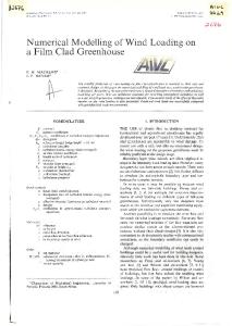
1. Introduction Disposal of wastewater with higher density than ambient water is a common phenomenon all over the world. Examples are the brine discharges from desalination plants and cooling water discharges from Liquefied Natural Gas (LNG) plants which can be seen in middle-eastern countries. The former has a good effect on the environment by decreasing exploitation of non-renewable water resources. However, at the same time it may cause negative local impacts on the environment (Bleninger and Jirka, 2008). The main issue is regarding the marine environment, especially for shoreline (Einav, 2003). Seawater desalination plants discharge a large volume of concentrated salt brine into the coastal waters (Fig. 1). There are other effluent discharges such as chemical wastes from biofouling (e.g. chlorine) and other substances which may result from fertilizers. Depending on the both discharge facility and ecological characteristics of the receiving water, those wastewaters can have a harmful impact on the local environment. For instance, areas such as coral reefs, mangrove forests, salt marshes, and generally low energy intertidal areas are very vulnerable (Hopner and Windelberg, 1996). Marine regions similar to Persian Gulf and Red Sea have low water exchange capacities and are less energetic, consequently more sensitive to desalination plants' discharges. Environmental impacts of effluent discharge into coastal waters include local fisheries potential, tourism industry, and other economic consequences. Genthner (2005) noted that the public and scientific concerns have been increased on the environmental impacts of the desalination plants recently. Therefore the mixing and dispersion mechanism of effluent discharges into ambient water has been studied by many researchers that would be briefly reviewed in continue. 51-1

Fig. 1. Al-Ghubrah desalination plant (largest in Oman) with a surface discharge (photo: H.H. Al-Barwani).

Cipolina et al. (2005), studied the dense jet in a still ambient to investigate flow behaviour at different inclinations, 30°, 45°, and 60°. Their study mainly focused on the key geometrical properties of the inclined dense jets such as maximum height and point of impact. However, their study did not report any dilution measurements and only focused on the image processing of the jet trajectory. Kikkert et al. (2007) developed an analytical method to predict the behaviour of inclined dense discharges and compared the results to their own experiments as well as other previous studies. They studied the inclined jets up to 75° from horizontal. The integrated dilution values from their study showed that the normalized dilution at terminal rise height is about the same for angles between 30° and 60°. This result is different from the earlier study by Zeitoun et al. (1970), but is supported by predictions of CORJET model (Jirka, 2004, 2008) which shows that the dilution value is almost the same at the terminal rise height of jets with inclination from 30° to 45°, with a higher value for 45° jets. This conclusion was made earlier by Cederwall (1968) in the stationary ambient water. More recently, Shao and Law (2010) conducted experiments on lower angles, 30° and 45° jets, with a combined Planar Laser Induced Fluorescent (PLIF) and Particle Image Velocimetry (PIV). They divided the experiments into two series: series F, in which the nozzle is placed far from the boundary (seabed), and series N, for cases close to the bottom boundary. The Coanda effect (see e.g. Shao and Law, 2010) was investigated in their study as well. Papakonstantis et al. (2011a) measured the trajectory characteristics of dense jets with ϴ=45° to 90° visually. The turbulent concentration fluctuation (Crms) measurements across a dense jet have been also studied for the jet angles ϴ=45°, 60° and 75° (Papakonstantis et al., 2011b). Lai and Lee (2012) reported a comprehensive experimental investigation of the tracer concentration field of inclined dense jets for jet densimetric Froude number of Fr=10 to 40 and a broad range of ϴ=15° to 60°. Empirical correlation of the terminal rise height, impact point and their dilution as a function of jet discharge angle were compared with prediction of VISJET model (Lee and Chu, 2003) as well as other data in their study. All above-mentioned studies are experimental. However, numerical modelling of dense jets has been started more recently, and hence requires more investigation and development. Kim et al. (2002) investigated the mixing processes of a buoyant jet discharged from a submerged single port using a threedimensional hybrid model. In the proposed hybrid model, the initial mixing was simulated by a jet integral method, and the advection-diffusion process was simulated using a particle tracking method. The proposed model was verified with their laboratory experiments which were conducted for various conditions. Vafeiadou et al. (2005) studied inclined negatively buoyant jets numerically using a threedimensional model (CFX-5). For turbulence closure, the SST (Shear Stress Transport) model was employed, which is based on a blending between the k-ε and the k-ω models. They used an unstructured grid with refinement near the bottom, where the boundary layer develops, and around the inflow nozzle. 51-2

They concluded that the model underestimated slightly the terminal rise height and considerably the return point compared to experimental data by Roberts et al. (1997). Oliver et al. (2008) investigated the geometrical and mixing characteristics of inclined dense jets using CFX model. They used the standard kε turbulence model as well as the one they calibrated through adjustment of the turbulent Schmidt number in the tracer transport equation. More recently, Elhaggag et al. (2011) studied dense brine jets both experimentally and numerically. However, they focused only on the vertical dense jets, and no inclination is reported in their investigation. The numerical simulations were conducted via a FLUENT CFD package and were compared to those from their experimental study.

2. Dimensional Analysis The sketch of the problem has been shown in Fig. 2. As seen in the figure, fluid of density ρ0 is issued to the stationary ambient from an inclined nozzle. The diameter of the nozzle is D at an angle ϴ and the ambient water density is ρa (ρa < ρ0). The jet reaches initially to a maximum height (initial terminal height). When the flow reaches to the steady state, the terminal rise height is reduced to a final value (terminal rise height) Yt. This height appears at a horizontal distance Xm from the nozzle, whereas Xr is the horizontal distance from the nozzle to the jet centerline at the source elevation.

Fig. 2. Inclined jet dispersion into ambient water.

With a full turbulent flow and assuming the Boussinesq approximation (ρ0-ρa) > 1 or Fr0 >> 1, the initial volume flux becomes unimportant (Fischer et al. 1979). Therefore, for a specific angle ϴ, dimensional analysis leads to the following expression for any length parameter, for example the rise height (Zeitoun et al., 1970; Roberts and Toms, 1987; Roberts et al., 1997)

Y  cons. DFr0

(7)

Above expression holds for any geometrical characteristic as following

Yt  C1 ( ) DFr0 Xm  C2 ( ) DFr0 Xr  C3 ( ) DFr0

(8) (9) (10)

These values have been calculated numerically and are presented in this paper for different angles.

3. Governing Equations The governing equations are the well-known Navier-Stokes equations for three-dimensional, incompressible fluids, as follows Continuity equation:

u v w   0 x y z

(11)

Momentum equations:

u u u u 1 P    u      u      u   u v w    eff     eff     eff    t x y z  x x   x   y   y   z   z  

(12)

v v v v 1 P    v      v      v     0 u v w    eff     eff     eff     g t x y z  y x   x   y   y   z   z   

(13)

w w w w 1 P    w      w      w   u v w    eff     eff     eff    t x y z  z x   x   y   y   z   z  

(14)

where u, v, and w are the mean velocity components in the x, y, and z directions, respectively, t is the time, P is the fluid pressure, υeff represents the effective kinematic viscosity (υeff=υt+υ), υt is the turbulent 51-4

kinematic viscosity, g is the gravity acceleration, ρ is the fluid density, and ρ0 is the reference fluid density. One should note that the equations are divided by density (ρ), and the buoyancy term is added to the momentum equation in the vertical direction (y-coordinate) to account for variable density effects. The time-history of the concentration and temperature are modelled using the advection-diffusion equation, as

  2C  2C  2C  C C C C u v w  D 2  2  2  t x y z y z   x 2 2   T  T  2T  T T T T u v w  keff  2  2  2  t x y z y z   x

(15)

(16)

with

keff 

t Prt





(17)

Pr

where C is the fluid concentration (salinity, S), D is the diffusion coefficient, T is the fluid temperature, keff is the heat transfer coefficient, Pr is the Prandtl number, and Prt is the turbulent Prandtl number. Turbulent Prandtl number was changed within the regular range 0.6-1 and it was numerically found that the results are insensitive to the turbulent Prandtl number within this range.

4. Results As mentioned before, four different cases have been studied for each angle in this paper. The cases are kept similar for three before-mentioned angles. These four cases are summarized in Table 1. Table 1. Parameters of numerical simulations. Test #

Inclined Angle ϴ

Inlet Diameter D (mm)

Initial Inlet Height Y0 (mm)

Δρ/ρa (%)

Discharge Velocity U0 (m/s)

Densimetric Froude # Fr0

1 2 3 4

60, 80, 85 60, 80, 85 60, 80, 85 60, 80, 85

10.65 10.65 10.65 10.65

8.155 8.155 8.155 8.155

1.983 2.646 1.865 2.084

1.173 0.973 1.044 0.588

25.77 18.50 36.90 12.60

4. 1. Terminal Rise Height The terminal rise height in steady state flow, normalized by the jet diameter D is plotted against Fr0 in Fig. 3 for each discharge angle. The numerical results confirm the dimensional analysis presented before. The model results are very close to each other for the two turbulence models and are consistent with the experimental data trend line. As shown in Fig. 3, the terminal rise height difference between the jet angles 80° and 85° is small due to small difference in inclination. However, it is noteworthy that the terminal rise height for 85° inclined dense jets is not necessarily larger than 80° jets. The same pattern is reported by Papakonstantis et al. (2011a).

51-5

140

Exp. 45 (Papakonstantis et al., 2011a) Exp. 60 (Papakonstantis et al., 2011a) Exp. 80 (Papakonstantis et al., 2011a) Exp. 85 (Papakonstantis et al., 2011a) Present Study, 60 Present Study, 80 Present Study, 85

120 100

140

realizable k-ε

Exp. 45 (Papakonstantis et al., 2011a) Exp. 60 (Papakonstantis et al., 2011a) Exp. 80 (Papakonstantis et al., 2011a) Exp. 85 (Papakonstantis et al., 2011a) Present Study, 60 Present Study, 80 Present Study, 85

120 100 80

Yt/D

Yt/D

80

LRR

60

60

40

40

20

20

0

0 0

20

40

60

Fr0

80

0

10

20

30

40

Fr0

50

60

70

Fig. 3. Normalized terminal rise height vs. Fr0 for realizable k-ε and LRR turbulence models, case #1.

4. 2. Horizontal Distance to the Jet Centerline Pick The jet centerline peak is defined from the centerline trajectory. The horizontal location of the jet centerline peak Xm is normalized by the nozzle diameter and is plotted versus the jet angle, ϴ, as shown in Fig. 4. Similar to the results presented in the above section, the two turbulence models are close to each other and the results are consistent with the experimental data. The numerical results for both realizable kε and LRR turbulence models are closer to the experimental data reported by Kikkert (2006) and Papakonstantis et al. (2011a) than the results presented by Cipolina et al. (2005). As seen in Fig. 4, for higher inclinations than 60° there is not a comprehensive data set. It is therefore important to investigate the inclinations higher than 60° and lower than 90°. Obviously, when the angle is increased the centerline peak is seen in the shorter distance from the source. 2.5

2.5

realizable k-ε

1.5

1.5

Xm/DFr0

2

Xm/DFr0

2

Exp. (Papakonstantis, 2011a) Exp. (Cipolina et al., 2005) Exp. (Kikkert LA, 2006) Exp. (Kikkert LIF, 2006) Present Study, 60 Present Study, 80 Present Study, 85

1

0.5

0

LRR

Exp. (Papakonstantis, 2011a) Exp. (Cipolina et al., 2005) Exp. (Kikkert LA, 2006) Exp. (Kikkert LIF, 2006) Present Study, 60 Present Study, 80 Present Study, 85

1

0.5

0 45

55

65

75

85

45

ϴ (deg)

55

65

ϴ (deg)

75

85

Fig. 4. Normalized horizontal location of centerline peak vs. ϴ for realizable k-ε and LRR turbulence models.

4. 3. Horizontal Distance to the Jet Return Point The return point is defined as the point at which the dense jet passes the nozzle tap elevation when it is falling in the descending part of the jet. It is different from the impact point if the nozzle tap is placed above the bottom surface (as is the case in this study) or if the bottom is sloped. The impact point is very important and has been broadly investigated in previous studies (Roberts et al., 1997; Cipolina et al., 2005; Jirka, 2008), since it is the point that mixing and water entrainment is significantly reduced and the effluent remains attached to the bed afterwards. After this point, the plume is dispersed as a bottom dense 51-6

current. However, the location of the impact point is dependent on the source height and bed slope, and therefore is very site-specific. Hence, the return point, which is independent of the source elevation and bed slope, is discussed in this paper for more generality. Since the practical nozzle height and the bed slope are typically small relative to the entire mixing zone that the jet passes through before reaching the return point, and therefore the distance between the return point and the impact point is not significant, so the return point can be used as a substitute for the impact point for practical purposes. The normalized horizontal distance from the nozzle to the point that jet returns at the elevation of the source, Xr/DFr0, is plotted in Fig. 5 versus the jet angle for realizable k-ε and LRR turbulence models. The results from present study are in good agreement with experimental data for both turbulence models. As Kheirkhah (2013) discussed, RSMs account automatically for the effects of the stress anisotropy which are important for the stress-induced secondary flows, as well as for the changes in the streamline trajectory (Hanjalic, 1994). This can result in a more accurate calculation of stresses, especially on the jetambient interface, where the pressure difference is present and controls the jet trajectory. As the RSMs consider different viscosity values for each direction, the jet behaviour can be calculated more accurately using these models. 4

4

realizable k-ε

3

3

2.5

2.5

Xr/DFr0

3.5

Xr/DFr0

3.5

2 Exp. (Papakonstantis et al., 2011a)

1.5

LRR

2

1.5

Exp. (Papakonstantis et al., 2011a)

Exp. (Zeitoun et al., 1970)

1 0.5

Present Study, 60

Present Study, 80

0.5

Present Study, 85

0 30

40

50

Exp. (Zeitoun et al., 1970)

1

Present Study, 60

Present Study, 80 Present Study, 85

0 60

70

80

90

ϴ (deg)

30

40

50

60

70

80

90

ϴ (deg)

Fig. 5. Normalized horizontal location of return point vs. ϴ for realizable k-ε and LRR turbulence models.

5. Conclusions Based on the dimensional analysis it is well-known that, the geometrical characteristics of the trajectory of a momentum-driven negatively buoyant jet normalized by the jet diameter D and the densimetric Froude number Fr0 take constant values for any specific discharge angle. An extensive numerical study was conducted using the Froude number ranging from 12.6 to 36.9 in order to characterize the geometrical properties of inclined negatively buoyant jets. Three discharge angles, 60°, 80°, and 85° have been chosen since these angles have not been studied comprehensively yet. Most previous studies focused on the vertical jets as well as the jets with lower inclinations. The numerical results confirmed the theoretical model and allowed the determination of the respective constants (C1, C2, and C3). The values obtained in this study have been compared to the previous experimental data. Reasonable agreement for these parameters was found between the current numerical study and previous experimental studies. However, the predicted terminal rise height is about 5% less than experimental data. Moreover, this study confirms that the terminal rise height for 80° jets is higher than 85° jets as previously reported by Bloomfield and Kerr (2002) and Papakonstantis et al. (2011). It was found that the realizable k-ε (an LEVM) and LRR (an RSM) turbulence models tend to be accurate turbulence models for the application of brine discharges studied herein. RSMs (mainly the LRR model) could successfully capture secondary flows and buoyancy-induced forces since these models account for the effects of the stress anisotropy (Kheirkhah Gildeh et al., 2013 and 2014). However, the 51-7

computational costs of the different turbulence models available have to be considered as well. RSMs are more computationally expensive than the LEVMs (about 20-25% more than LEVMs), and thus need more computational recourses. More inclinations in the range of 60° and 90° should be studied in brine discharges from desalination plants. The two turbulence models used here are currently being utilized to do more parametric studies on inclined dense jets by the authors. Acknowledgements This publication was made possible by NPRP grant # 4-935-2-354 from the Qatar National Research Fund (a member of Qatar Foundation). The statements made herein are solely the responsibility of the authors.

References Bleninger T., Jirka G.H. (2008). Modeling and environmentally sound management of brine discharges from desalination plants. Desal., 221, 585-597. Bloomfield L.J., Kerr R.C. (2002). Inclined turbulent fountains. J. Fluid Mech., 451: 283-294. Cederwall K. (1968). Hydraulics of marine waste water disposal. Chalmers Inst. Tech. Cipollina A., Brucato A., Grisafi F., Nicosia S. (2005). Bench-scale investigation of inclined dense jets. J. Hydraul. Eng., 131(11): 1017–1022. Einav R. (2003). Checking today's brine discharges can help plan tomorrows plants. Desal. Wat. Reuse, 13 (1): 16–20. Elhaggag M.E., Elgamal M.H., Farouk M.I. (2011). Experimental and numerical investigation of desalination plant outfalls in limited disposal areas. J. Environ. Protec., 2:828-839. Fischer H.B., List E.J., Koh R.C.Y., Imberger J., Brooks N.H. (1979). Mixing in inland and coastal waters. Academic Press, New York. Genthner K. (2005). Research and Development in Desalination–Current Activities and Demand, in Lecture Notes. DME Seminar, Berlin. Hanjalic K. (1994). Advanced turbulence closure models: a view of current status and future prospects. Int. J. Heat and Fluid Flow. 15(3):178-203. Höpner T., Windelberg, J. (1996). Elements of environmental impact studies on coastal desalination plants. Desalination. 108 (1996) 11–18. Jirka G.H. (2004). Integral model for turbulent buoyant jets in unbounded stratified flows. Part I: the single round jet. Env. Fluid Mech. 4:1-56. Jirka G.H. (2008). Improved discharge configurations for brine effluents from desalination plants. J. Hydraul. Eng., ASCE. 134(1):116-120. Kheirkhah Gildeh H. (2013). Numerical Modeling of Thermal/Saline Discharges in Coastal Waters. MASc thesis. University of Ottawa, Ottawa, ON, Canada. Kheirkhah Gildeh H., Mohammadian A., Nistor I., Qiblawey H. (2014). Numerical Modeling of Turbulent Buoyant Wall Jets in Stationary Ambient Water. J. Hydraul. Eng., 10.1061/(ASCE)HY.19437900.0000871, 04014012. Kikkert G.A., Davidson M.J., Nokes R.I. (2007). Inclined negatively buoyant discharge. J. Hydraul. Eng., ASCE. 133(5):545-554. Kim D.G., Cho H.Y. (2006). Modeling the buoyant flow of heated water discharged from surface and submerged side outfalls in shallow and deep water with a cross flow. J. Environ. Fluid Mech. 6:501-518. Lai C.C.K., Lee J.H.W. (2012). Mixing of inclined dense jets in stationary ambient. J. Hydro-environ. Res. 6: 9-28. Lee J.H.W., Chu V.H. (2003). Turbulent jets and plumes: a lagrangian approach. Academic Publishers, the Netherland. Oliver C.J., Davidson M.J., Nokes R.I. (2008). k-ε prediction of the initial mixing of desalination discharges. J. Environ. Fluid Mech. 8:617-625. Papakonstantis I.G., Christodoulou G.C., Papanicolaou P.N. (2011a). Inclined negatively buoyant jets 1: geometrical characteristics. J. Hydraulic Res. 49(1): 3–12.

51-8

Papakonstantis I.G., Christodoulou G.C., Papanicolaou P.N. (2011b). Inclined negatively buoyant jets 2: concentration measurements. J. Hydraulic Res. 49(1): 13–22. Roberts P.J.W., Ferrier A., Daviero G. (1997). Mixing in inclined dense jets. J. Hydraul. Eng., ASCE. 123(8): 693–699. Roberts P.J.W., Toms G. (1987). Inclined dense jets in flowing current. J. Hydraul. Eng., ASCE. 113(3):323341. Shao D., Law A.W.K. (2010). Mixing and boundary interactions of 30 and 45 inclined dense jets. Env. Fluid Mech. 10:521-553. Vafeiadou P., Papakonstantis I., Christodoulou G. (2005). Numerical simulation of inclined negatively buoyant jets. The 9th international conference on environmental science and technology, September 1-3, Rhodes island, Greece. Zeitoun M.A., McIlhenny W.F., Reid R.O. (1970). Conceptual designs of outfall systems for desalting plants. Res. and Devel. Progress Report 550, Office of Saline Water, US Dept. of Interior, Washington DC.

51-9