Motivation: pricing and hedging of derivatives Pathwise calculus for non-anticipative flows Functional change of variable formulas Functional Ito calculus Martingale representation and hedging formulas Extensions Functional equations for martingales
Non-anticipative functional calculus and applications Spring School on Stochastic Processes, Thuringia, March 2011
Rama Cont
Laboratoire de Probabilit´es et Mod`eles Al´eatoires CNRS -Universit´e de Paris VI and Columbia University, New York Joint work with: David Fourni´e (Columbia University) Rama Cont
Functional Ito calculus
Motivation: pricing and hedging of derivatives Pathwise calculus for non-anticipative flows Functional change of variable formulas Functional Ito calculus Martingale representation and hedging formulas Extensions Functional equations for martingales
Outline Motivation: path-dependent derivatives. Adapted processes as non-anticipative flows. Functional calculus: horizontal and vertical derivatives. A pathwise change of variable formula for functionals. A functional Ito formula for semimartingales. Martingale representation formula I: regular case. A universal hedging formula for path-dependent options Weak derivative. Integration by parts formula. Martingale representation formula II: general case. Numerical computation of hedging strategies. Martingales as solutions to functional equations. A universal pricing equation for path-dependent options. Example: Asian options. Rama Cont
Functional Ito calculus
Motivation: pricing and hedging of derivatives Pathwise calculus for non-anticipative flows Functional change of variable formulas Functional Ito calculus Martingale representation and hedging formulas Extensions Functional equations for martingales
References Dupire, B. (2009) Functional Ito calculus, SSRN Preprint. R. Cont & D Fourni´e (2010) A functional extension of the Ito formula, Comptes Rendus Acad. Sci., Vol. 348, 57–61. R. Cont & D Fourni´e (2009) Functional Ito formula and stochastic integral representation of martingales, arxiv/math.PR. R. Cont & D Fourni´e (2010) Change of variable formulas for non-anticipative functionals on path space, Journal of Functional Analysis, Vol 259, 1043–1072. R. Cont (2010) Martingale representation formulas for Poisson random measures, Working Paper. R Cont (2010) Pathwise computation of hedging strategies for path-dependent derivatives, Working Paper. Rama Cont
Functional Ito calculus
Motivation: pricing and hedging of derivatives Pathwise calculus for non-anticipative flows Functional change of variable formulas Functional Ito calculus Martingale representation and hedging formulas Extensions Functional equations for martingales
Motivation: modeling of derivative securities Mathematical models of financial markets model uncertainty by representing future evolution of prices in terms of a filtered scenario space (Ω, ℱ, ℱt )t∈[0,T ] ) and an ℱt −adapted price process S : [0, T ] × Ω 7→ ℝd where Ω represents the set of market scenarios ℱ represents the set of market events (which we can make sense of) ℱt represents the information revealed at date t, and S(t, 𝜔) = (S 1 (t, 𝜔), .., S d (t, 𝜔)) represents the prices of securities at date t in scenario 𝜔. Specifying a probability measure ℙ gives a filtered probability space but there is often no consensus about the specification of ℙ: model uncertainty. Rama Cont
Functional Ito calculus
Motivation: pricing and hedging of derivatives Pathwise calculus for non-anticipative flows Functional change of variable formulas Functional Ito calculus Martingale representation and hedging formulas Extensions Functional equations for martingales
Contingent claims A contingent claim or derivative security on S is given by a (ℱT -measurable) payoff H : Ω 7→ ℝ Call option: H(𝜔) = (S(T , 𝜔) − K )+ ∫T Asian option: H(𝜔) = ( T1 0 S(t, 𝜔) dt − K )+ Barrier option: knockout call H(𝜔) = 1maxt∈[0,T ] S(t,𝜔) 0, ∀h ∈ [0, t],
∀𝜔 ′ ∈ D([0, t − h], ℝd ),
d∞ (𝜔, 𝜔 ′ ) < 𝜂 ⇒ ∣Ft (𝜔) − Ft−h (𝜔 ′ )∣ < 𝜖 Rama Cont
Functional Ito calculus
Motivation: pricing and hedging of derivatives Pathwise calculus for non-anticipative flows Functional change of variable formulas Functional Ito calculus Martingale representation and hedging formulas Extensions Functional equations for martingales
Functional representation of non-anticipative processes Horizontal derivative Vertical derivative of a functional Spaces of regular flows Examples Obstructions to regularity Non-uniqueness of functional representation
Boundedness-preserving flows We call a flow “boundedness preserving” if it is bounded on each bounded set of paths: Definition (Boundedness-preserving flows) Define 𝔹([0, T )) as the set of non-anticipative flows F on Υ([0, T ]) such that for every compact subset K of ℝd , every R > 0 and t0 < T ∃CK ,R,t0 > 0,
∀t ≤ t0 ,
∀𝜔 ∈ D([0, t], K ),
sup ∣v (s)∣ ≤ R ⇒ ∣Ft (𝜔)∣ ≤ CK ,R,t0 s∈[0,t]
Rama Cont
Functional Ito calculus
Motivation: pricing and hedging of derivatives Pathwise calculus for non-anticipative flows Functional change of variable formulas Functional Ito calculus Martingale representation and hedging formulas Extensions Functional equations for martingales
Functional representation of non-anticipative processes Horizontal derivative Vertical derivative of a functional Spaces of regular flows Examples Obstructions to regularity Non-uniqueness of functional representation
Measurability and continuity A non-anticipative flow F = (Ft ) applied to X generates an ℱt −adapted process Y (t) = Ft ({X (u), 0 ≤ u ≤ t}) = Ft (Xt ) Theorem Let 𝜔 ∈ D([0, T ], ℝd ). If F ∈ ℂ0,0 l , the path t 7→ Ft (𝜔t− ) is left-continuous. Y (t) = Ft (Xt ) defines a predictable process.
Rama Cont
Functional Ito calculus
Motivation: pricing and hedging of derivatives Pathwise calculus for non-anticipative flows Functional change of variable formulas Functional Ito calculus Martingale representation and hedging formulas Extensions Functional equations for martingales
Functional representation of non-anticipative processes Horizontal derivative Vertical derivative of a functional Spaces of regular flows Examples Obstructions to regularity Non-uniqueness of functional representation
Definition (Horizontal derivative) We say that a non-anticipative flow F = (Ft )t∈[0,T ] is horizontally differentiable at 𝜔 ∈ D([0, t], ℝd ) if 𝒟t F (𝜔) = lim+ h→0
Ft+h (𝜔t,h ) − Ft (𝜔) h
exists
We will call 𝒟t F (𝜔) the horizontal derivative 𝒟t F of F at 𝜔. By right continuity of (ℱt ), 𝒟t F is ℱt -measurable: 𝒟F = (𝒟t F )t∈[0,T ] defines a non-anticipative flow. If Ft (𝜔) = f (t, 𝜔(t)) with f ∈ C 1,1 ([0, T ] × ℝd ) then 𝒟t F (𝜔) = ∂t f (t, 𝜔(t)). Rama Cont
Functional Ito calculus
Motivation: pricing and hedging of derivatives Pathwise calculus for non-anticipative flows Functional change of variable formulas Functional Ito calculus Martingale representation and hedging formulas Extensions Functional equations for martingales
Functional representation of non-anticipative processes Horizontal derivative Vertical derivative of a functional Spaces of regular flows Examples Obstructions to regularity Non-uniqueness of functional representation
Vertical perturbation of a path 3
2.5
2
1.5
1
0.5
0
−0.5
0
0.1
0.2
0.3
0.4
0.5
0.6
0.7
0.8
0.9
1
Figure: For e ∈ ℝd , the vertical perturbation 𝜔te of 𝜔t is the cadlag path obtained by shifting the endpoint: 𝜔te (u) = 𝜔(u) for u < t and 𝜔te (t) = 𝜔(t) + e.
Rama Cont
Functional Ito calculus
Motivation: pricing and hedging of derivatives Pathwise calculus for non-anticipative flows Functional change of variable formulas Functional Ito calculus Martingale representation and hedging formulas Extensions Functional equations for martingales
Functional representation of non-anticipative processes Horizontal derivative Vertical derivative of a functional Spaces of regular flows Examples Obstructions to regularity Non-uniqueness of functional representation
Definition A non-anticipative flow F = (Ft )t∈[0,T [ is said to be vertically differentiable at 𝜔 ∈ D([0, t]), ℝd ) if ℝd
7→ ℝ
e → Ft (𝜔t + e1t ) is differentiable at 0. Its gradient at 0 is called the vertical derivative of Ft at 𝜔: ∇𝜔 Ft (𝜔) = (∂i Ft (𝜔), i = 1..d) ∂i Ft (𝜔) = lim
h→0
Rama Cont
where
Ft (𝜔thei )
− Ft (𝜔) h
Functional Ito calculus
Motivation: pricing and hedging of derivatives Pathwise calculus for non-anticipative flows Functional change of variable formulas Functional Ito calculus Martingale representation and hedging formulas Extensions Functional equations for martingales
Functional representation of non-anticipative processes Horizontal derivative Vertical derivative of a functional Spaces of regular flows Examples Obstructions to regularity Non-uniqueness of functional representation
Vertical derivative of a flow ∇𝜔 Ft (𝜔).e is simply a directional derivative in the direction of the indicator function 1{t} e. Note that to compute ∇𝜔 Ft (𝜔) we need to compute F outside C0 : even if 𝜔 ∈ C0 , 𝜔th ∈ / C0 . ∇𝜔 Ft (𝜔) is ’local’ in the sense that it is computed for t fixed and involves perturbing the endpoint of paths ending at t. ∇𝜔 F = (∇𝜔 Ft )t∈[0,T ] is a non-anticipative flow. This derivative was introduce by B. Dupire to compute the sensitivity of an option price to its underlying.
Rama Cont
Functional Ito calculus
Motivation: pricing and hedging of derivatives Pathwise calculus for non-anticipative flows Functional change of variable formulas Functional Ito calculus Martingale representation and hedging formulas Extensions Functional equations for martingales
Functional representation of non-anticipative processes Horizontal derivative Vertical derivative of a functional Spaces of regular flows Examples Obstructions to regularity Non-uniqueness of functional representation
Spaces of differentiable flows Definition (Spaces of differentiable functionals) 0,0 For j, k ≥ 1 define ℂj,k b ([0, T ]) as the set of functionals F ∈ ℂr which are differentiable j times horizontally and k times vertically at all 𝜔 ∈ D([0, t], ℝd ), t < T , with
horizontal derivatives 𝒟tm F , m ≤ j continuous on D([0, T ]) for each t ∈ [0, T [ left-continuous vertical derivatives: ∀n ≤ k, ∇n𝜔 F ∈ ℂl0,0 . 𝒟tm F , ∇n𝜔 F ∈ 𝔹([0, T ]). We can have F ∈ ℂ1,1 echet differentiable b ([0, T ]) while Ft not Fr´ for any t ∈ [0, T ]. Rama Cont
Functional Ito calculus
Motivation: pricing and hedging of derivatives Pathwise calculus for non-anticipative flows Functional change of variable formulas Functional Ito calculus Martingale representation and hedging formulas Extensions Functional equations for martingales
Functional representation of non-anticipative processes Horizontal derivative Vertical derivative of a functional Spaces of regular flows Examples Obstructions to regularity Non-uniqueness of functional representation
Examples of regular functionals Example (Cylindrical functionals) For g ∈ C 0 (ℝd ), h ∈ C k (ℝd ) with h(0) = 0. Then Ft (𝜔) = h (𝜔(t) − 𝜔(tn −))
1t≥tn
g (𝜔(t1 −), 𝜔(t2 −)..., 𝜔(tn −))
is in ℂb1,k and 𝒟t F (𝜔) = 0,
and
∇j𝜔 Ft (𝜔) = h(j) (𝜔(t) − 𝜔(tn −))
Rama Cont
∀j = 1..k, 1t≥tn g (𝜔(t1 −), 𝜔(t2 −)..., 𝜔(tn −))
Functional Ito calculus
Motivation: pricing and hedging of derivatives Pathwise calculus for non-anticipative flows Functional change of variable formulas Functional Ito calculus Martingale representation and hedging formulas Extensions Functional equations for martingales
Functional representation of non-anticipative processes Horizontal derivative Vertical derivative of a functional Spaces of regular flows Examples Obstructions to regularity Non-uniqueness of functional representation
Examples of regular functionals Example (Integral functionals) ∫t For g ∈ C0 (ℝd ), Y (t) = 0 g (X (u))𝜌(u)du = Ft (Xt ) where ∫ Ft (𝜔) =
t
g (𝜔(u))𝜌(u)du 0
F ∈ ℂ1,∞ b , with: 𝒟t F (𝜔) = g (𝜔(t))𝜌(t)
Rama Cont
∇j𝜔 Ft (𝜔) = 0
Functional Ito calculus
Motivation: pricing and hedging of derivatives Pathwise calculus for non-anticipative flows Functional change of variable formulas Functional Ito calculus Martingale representation and hedging formulas Extensions Functional equations for martingales
Functional representation of non-anticipative processes Horizontal derivative Vertical derivative of a functional Spaces of regular flows Examples Obstructions to regularity Non-uniqueness of functional representation
Obstructions to regularity Example (Jump of x at the current time) Ft (𝜔) = 𝜔(t) − 𝜔(t−) has regular pathwise derivatives: 𝒟t F (𝜔) = 0
∇𝜔 Ft (𝜔) = 1
But F ∈ / ℂr0,0 ∪ ℂ0,0 l . Example (Jump of x at a fixed time) Ft (𝜔) = 1t≥t0 (𝜔(t0 ) − 𝜔(t0 −)) F ∈ ℂ0,0 has horizontal and vertical derivatives at any order, but ∇𝜔 Ft (𝜔) = 1t=t0 fails to be left (or right) continuous. Rama Cont
Functional Ito calculus
Motivation: pricing and hedging of derivatives Pathwise calculus for non-anticipative flows Functional change of variable formulas Functional Ito calculus Martingale representation and hedging formulas Extensions Functional equations for martingales
Functional representation of non-anticipative processes Horizontal derivative Vertical derivative of a functional Spaces of regular flows Examples Obstructions to regularity Non-uniqueness of functional representation
Obstructions to regularity
Example (Maximum) Ft (𝜔) = sups≤t 𝜔(s) F ∈ ℂ0,0 but is not vertically differentiable on {𝜔 ∈ D([0, t], ℝd ),
Rama Cont
𝜔(t) = sup 𝜔(s)}. s≤t
Functional Ito calculus
Motivation: pricing and hedging of derivatives Pathwise calculus for non-anticipative flows Functional change of variable formulas Functional Ito calculus Martingale representation and hedging formulas Extensions Functional equations for martingales
Functional representation of non-anticipative processes Horizontal derivative Vertical derivative of a functional Spaces of regular flows Examples Obstructions to regularity Non-uniqueness of functional representation
Non-uniqueness of functional representation Given a process Y (say, the value of a path dependent option If F 1 , F 2 ∈ ℂ1,1 coincide on continuous paths ∀t < T ,
∀𝜔 ∈ C0 ([0, t], ℝd ), Ft1 (𝜔) = Ft2 (𝜔)
then ℙ(∀t ∈ [0, T ], F 1 (Xt ) = F 2 (Xt ) ) = 1 Yet, ∇𝜔 F depends on the values of F computed at discontinuous paths...
Rama Cont
Functional Ito calculus
Motivation: pricing and hedging of derivatives Pathwise calculus for non-anticipative flows Functional change of variable formulas Functional Ito calculus Martingale representation and hedging formulas Extensions Functional equations for martingales
Functional representation of non-anticipative processes Horizontal derivative Vertical derivative of a functional Spaces of regular flows Examples Obstructions to regularity Non-uniqueness of functional representation
Derivatives of flows defined on continuous paths Theorem If F 1 , F 2 ∈ ℂ1,1 coincide on continuous paths ∀t < T ,
∀𝜔 ∈ C0 ([0, t], ℝd ), Ft1 (𝜔t ) = Ft2 (𝜔t )
then their pathwise derivatives also coincide: ∀t < T , ∇𝜔 Ft1 (𝜔t ) = ∇𝜔 Ft2 (𝜔t ),
Rama Cont
∀𝜔 ∈ C0 ([0, t], ℝd ), 𝒟t Ft1 (𝜔t ) = 𝒟t Ft2 (𝜔t )
Functional Ito calculus
Motivation: pricing and hedging of derivatives Pathwise calculus for non-anticipative flows Functional change of variable formulas Functional Ito calculus Martingale representation and hedging formulas Extensions Functional equations for martingales
Paths of finite quadratic variation A pathwise change of variable formula for functionals Ito-F¨ ollmer integral
Quadratic variation for cadlag paths [F¨ollmer (1979)] x ∈ D([0, T ], ℝ) has finite quadratic variation along the sequence k(n) of partitions 𝜋n = (0 = t0n < ..tn = T ) if the discrete measures k(n)−1 n
𝜉 =
∑
n (x(ti+1 ) − x(tin ))2 𝛿tin
i=0
converge weakly to some Radon measure 𝜉 on [0, T ]: ∫ k(n)−1 ∑ n→∞ n ) − x(tin ))2 f (tin ) → ∀f ∈ Cb0 (ℝ), (x(ti+1
T
0
i=0
In particular k(n)−1
∑
n→∞
n (x(ti+1 ) − x(tin ))2 → [x](t) := 𝜉([0, t])
i=0 Rama Cont
Functional Ito calculus
f
d𝜉
Motivation: pricing and hedging of derivatives Pathwise calculus for non-anticipative flows Functional change of variable formulas Functional Ito calculus Martingale representation and hedging formulas Extensions Functional equations for martingales
Paths of finite quadratic variation A pathwise change of variable formula for functionals Ito-F¨ ollmer integral
Quadratic variation for cadlag paths Denote Q([0, T ], 𝜋) the set of x ∈ D([0, T ], ℝd ) with finite quadratic variation with respect to the partition 𝜋 = (𝜋n )n≥1 . For x ∈ Q([0, T ], 𝜋), the increasing function k(n)−1
∑
n→∞
n (x(ti+1 ) − x(tin ))2 → [x](t) := 𝜉([0, t])
i=0
is called the quadratic variation of x along the partition (𝜋n ) and has Lebesgue decomposition ∑ [x](t) = [x]c (t) + (Δx(s))2 0 0. There exists a sequence of (random) partitions 𝜋 = (𝜋n )n≥1 of [0, T ], composed of 𝔽-stopping times, with ∣𝜋n ∣ → 0 a.s., such that the paths of S lie in Q([0, T ], 𝜋) with probability 1: ℙ({𝜔 ∈ Ω,
S(., 𝜔) ∈ Q([0, T ], 𝜋(𝜔))}) = 1.
Proof: take the dyadic partition tnk = kT /2n , k = 0..2n . Since ∑ n (S(tk+1 ) − S(tkn ))2 → [S] exists a ∑T in probability, there 2 subsequence 𝜋n such that 𝜋n (S(ti ) − S(ti+1 )) → [S]T a.s. Rama Cont
Functional Ito calculus
Motivation: pricing and hedging of derivatives Pathwise calculus for non-anticipative flows Functional change of variable formulas Functional Ito calculus Martingale representation and hedging formulas Extensions Functional equations for martingales
Paths of finite quadratic variation A pathwise change of variable formula for functionals Ito-F¨ ollmer integral
Change of variable for functionals of cadlag paths Let 𝜔 ∈ D([0, T ] × ℝd ) where 𝜔 has finite quadratic variation along (𝜋n ) and ∣𝜔(t) − 𝜔(t−)∣ → 0
sup t∈[0,T ]−𝜋n n − tn, Denote hin = ti+1 i k(n)−1
∑
n
𝜔 (t) =
𝜔(ti+1 −)1[ti ,ti+1 ) (t) + 𝜔(T )1{T } (t)
i=0
Consider the ’Riemann sum’: k(n)−1
∑
n,𝛿𝜔(tin )
∇𝜔 Ftin (𝜔t n − i
n n )(𝜔(ti+1 ) − 𝜔(tin )) 𝛿𝜔(tin ) = 𝜔(ti+1 ) − 𝜔(tin )
i=0 Rama Cont
Functional Ito calculus
Motivation: pricing and hedging of derivatives Pathwise calculus for non-anticipative flows Functional change of variable formulas Functional Ito calculus Martingale representation and hedging formulas Extensions Functional equations for martingales
Paths of finite quadratic variation A pathwise change of variable formula for functionals Ito-F¨ ollmer integral
A pathwise change of variable formula for functionals Theorem (R.C. & D Fourni´e (Jour. Func. Analysis 2010)) For any F ∈ ℂb1,2 ([0, T [), 𝜔 ∈ Q([0, T ], 𝜋) the F¨ ollmer integral ∫
k(n)−1
T 𝜋
∇𝜔 Ft (𝜔t− )d 𝜔 := lim
n→∞
0
∑
n,𝛿𝜔(tin )
∇𝜔 Ftin (𝜔t n − i
n )(𝜔(ti+1 ) − 𝜔(tin ))
i=0
∫ exists and FT (𝜔T ) − F0 (𝜔0 ) = ∫ + 0
T
T
𝒟t Ft (𝜔u− )du 0 T
∫ ) 1 (t 2 tr ∇𝜔 Ft (𝜔u− )d[𝜔]c (u) + ∇𝜔 Ft (𝜔t− )d 𝜋 𝜔 2 0 ∑ + [Fu (𝜔u ) − Fu (𝜔u− ) − ∇𝜔 Fu (𝜔u− ).Δ𝜔(u)] u∈]0,T ]
Rama Cont
Functional Ito calculus
Motivation: pricing and hedging of derivatives Pathwise calculus for non-anticipative flows Functional change of variable formulas Functional Ito calculus Martingale representation and hedging formulas Extensions Functional equations for martingales
Paths of finite quadratic variation A pathwise change of variable formula for functionals Ito-F¨ ollmer integral
Sketch of proof: continuous case 𝜔 ∈ C0 ([0, T ]) is (uniformly) continuous on [0, T ] so 𝜂n =
sup
n {∣𝜔(u) − 𝜔(tin )∣ + ∣ti+1 − tin ∣} → 0 n→∞
n ) 0≤i≤k(n)−1,u∈[tin ,ti+1
Consider the decomposition: n n (𝜔 n Fti+1 t
i+1 −
n n (𝜔 n ) − Ftin (𝜔tnn − ) = Fti+1 t
i+1 −
i
) − Ftin (𝜔tnn ) i
+ Ftin (𝜔tnn ) − Ftin (𝜔tnn − ) i
i
First term= 𝜓(hin ) − 𝜓(0) where 𝜓(u) = Ftin +u (𝜔tnn ,u ). i Since F ∈ ℂ1,2 ([0, T ]), 𝜓 is right-differentiable so n n (𝜔 n n ) Fti+1 ti ,hi
−
Ftin (𝜔tnn ) i
∫ =
Rama Cont
0
n −t n ti+1 i
𝒟tin +u F (𝜔tnn ,u )du i
Functional Ito calculus
Motivation: pricing and hedging of derivatives Pathwise calculus for non-anticipative flows Functional change of variable formulas Functional Ito calculus Martingale representation and hedging formulas Extensions Functional equations for martingales
Paths of finite quadratic variation A pathwise change of variable formula for functionals Ito-F¨ ollmer integral
Sketch of proof: continuous case The second term= 𝜙(𝛿𝜔in ) − 𝜙(0), where: 𝜙(u) = Ftin (𝜔tn,u n ). Since i − 1,2 2 F ∈ ℂ ([0, T ]), 𝜙 is C and: 𝜙′ (u) = ∇𝜔 Ftin (𝜔tn,u n−) i
𝜙′′ (u) = ∇2𝜔 Ftin (𝜔tn,u n−) i
Second order Taylor expansion of 𝜙 at u = 0: Ftin (𝜔tnn ) − Ftin (𝜔tnn − ) = ∇𝜔 Ftin (𝜔tnn − )𝛿𝜔in i i i ) 1 ( 2 + tr ∇𝜔 Ftin (𝜔tnn − ) t 𝛿𝜔in 𝛿𝜔in + rin i 2 n ) − 𝜔(t n ) and where 𝛿𝜔in = 𝜔(ti+1 i rin ≤ K ∣𝛿𝜔in ∣2
n,𝜔(t)−𝜔(tin )
sup t∈B(𝜔(tin ),𝜂n )
∣∇2𝜔 Ftin (𝜔t n −
Rama Cont
i
) − ∇2𝜔 Ftin (𝜔tnn − )∣
Functional Ito calculus
i
Motivation: pricing and hedging of derivatives Pathwise calculus for non-anticipative flows Functional change of variable formulas Functional Ito calculus Martingale representation and hedging formulas Extensions Functional equations for martingales
Paths of finite quadratic variation A pathwise change of variable formula for functionals Ito-F¨ ollmer integral
So finally we have the decomposition n n (𝜔 n Fti+1 t
i+1 −
∫
n ti+1
= tin
) − Ftin (𝜔tnn − ) i
𝒟u F (𝜔tnn ,u−t n )du + ∇𝜔 Ftin (𝜔tnn − )𝛿𝜔in i
i
i
1 + tr ∇2𝜔 Ftin (𝜔tnn − ) i 2 (
t
) 𝛿𝜔in 𝛿𝜔in + rin
n → ∞: n ∫Asti+1 ∫T n tin 𝒟u F (𝜔tin ,u−tin )du → 0 𝒟u F (𝜔u )du by dominated convergence. ∑ rin ≤ 𝜖ni ∣𝛿𝜔in ∣2 where C ≥ ∣𝜖ni ∣ → 0 so i rin → 0.
Rama Cont
Functional Ito calculus
Motivation: pricing and hedging of derivatives Pathwise calculus for non-anticipative flows Functional change of variable formulas Functional Ito calculus Martingale representation and hedging formulas Extensions Functional equations for martingales
Paths of finite quadratic variation A pathwise change of variable formula for functionals Ito-F¨ ollmer integral
A diagonal lemma Lemma (R.C. and D Fourni´e, 2010) Let (𝜇n )n≥1 be a sequence of Radon measures on [0, T ] converging weakly to a Radon measure 𝜇 with no atoms, and (fn )n≥1 , f be left-continuous functions on [0, T ] with ∀t ∈ [0, T ], lim fn (t) = f (t) n
then
∀t ∈ [0, T ], ∥fn (t)∥ ≤ K ∫ t ∫ t n→∞ fn d𝜇n → fd𝜇 s
s
So the sum of third terms converges to ∫ T ∫ T ) ) 1 (t 2 1 (t 2 tr ∇𝜔 Ft (𝜔u ).d[𝜔](u) = tr ∇𝜔 Ft (𝜔u ).d[𝜔](u) 0 2 0 2 Rama Cont
Functional Ito calculus
Motivation: pricing and hedging of derivatives Pathwise calculus for non-anticipative flows Functional change of variable formulas Functional Ito calculus Martingale representation and hedging formulas Extensions Functional equations for martingales
Paths of finite quadratic variation A pathwise change of variable formula for functionals Ito-F¨ ollmer integral
The F¨ollmer integral Since all other terms converge, we conclude that the limit ∫ 0
k(n)−1
T
∇𝜔 Ft (𝜔t− )d 𝜋 𝜔 := lim
n→∞
∑
n,Δ𝜔(tin )
∇𝜔 Ftin (𝜔t n − i
n )(𝜔(ti+1 )−𝜔(tin ))
i=0
exists pathwise. Such integrals were defined in [F¨ ollmer 1981] for integrands of the form f ′ (X (t)) where f ∈ C 2 (ℝd ). The construction depends a priori on the sequence 𝜋 of partitions. But, for semimartingales and, more generally, Dirichlet processes, one obtains a limit object which is a.s. independent of the choice of 𝜋. Rama Cont
Functional Ito calculus
Motivation: pricing and hedging of derivatives Pathwise calculus for non-anticipative flows Functional change of variable formulas Functional Ito calculus Martingale representation and hedging formulas Extensions Functional equations for martingales
Functional Functional Functional Functional
Ito formula: continuous case Ito formula: cadlag case Ito formula: proof of Dirichlet processes
Ito formula for functionals of semimartingales Applied to a semimartingale, these results lead to a functional extension of the Ito formula: Theorem (Functional Ito formula (R.C.& Fourni´e, 2009)) Let X be a continuous semimartingale and F ∈ ℂb1,2 ([0, T [). For any t ∈ [0, T [, ∫ t Ft (Xt ) − F0 (X0 ) = 𝒟u F (Xu )du + 0 ∫ t ∫ t ) 1 (t 2 ∇𝜔 Fu (Xu ).dX (u) + tr ∇𝜔 Fu (Xu ) d[X ](u) a.s. 0 0 2 In particular, Y (t) = Ft (Xt ) is a semimartingale. Rama Cont
Functional Ito calculus
Motivation: pricing and hedging of derivatives Pathwise calculus for non-anticipative flows Functional change of variable formulas Functional Ito calculus Martingale representation and hedging formulas Extensions Functional equations for martingales
Functional Functional Functional Functional
Ito formula: continuous case Ito formula: cadlag case Ito formula: proof of Dirichlet processes
Let X be a cadlag semimartingale and denote for t > 0, Xt− (u) = X (u)1[0,t) + X (t−)1t . Theorem (Functionals of cadlag semimartingales) For any F ∈ ℂb1,2 ([0, T [), t ∈ [0, T [, ∫
t
Ft (Xt ) − F0 (X0 ) = ∇𝜔 Fu (Xu ).dX (u) + 0 ∫ t ∫ t ) 1 (t 2 tr ∇𝜔 Fu (Xu ) d[X ](u) 𝒟u F (Xu )du + 0 0 2 ∑ + [Fu (Xu ) − Fu (Xu− ) − ∇𝜔 Fu (Xu− ).ΔX (u)]a.s. u∈]0,T ]
In particular, Y (t) = Ft (Xt ) is a semimartingale. Rama Cont
Functional Ito calculus
Motivation: pricing and hedging of derivatives Pathwise calculus for non-anticipative flows Functional change of variable formulas Functional Ito calculus Martingale representation and hedging formulas Extensions Functional equations for martingales
Functional Functional Functional Functional
Ito formula: continuous case Ito formula: cadlag case Ito formula: proof of Dirichlet processes
Functional Ito formula If Ft (Xt ) = f (t, X (t)) where f ∈ C 1,2 ([0, T ] × ℝd ) this reduces to the standard Ito formula. For F ∈ ℂ1,2 , Y (t) = Ft (Xt ) can be reconstructed from the ‘second-order jet’ (F , 𝒟F , ∇𝜔 F , ∇2𝜔 F ) of F along the path of X. If X has continuous paths then Y = F (X ) depends on F and its derivatives only via their values on continuous paths: Y can be∪reconstructed from the second-order jet of F on Υc = t∈[0,T ] C0 ([0, t], ℝd ) ⊂ Υ.
Rama Cont
Functional Ito calculus
Motivation: pricing and hedging of derivatives Pathwise calculus for non-anticipative flows Functional change of variable formulas Functional Ito calculus Martingale representation and hedging formulas Extensions Functional equations for martingales
Functional Functional Functional Functional
Ito formula: continuous case Ito formula: cadlag case Ito formula: proof of Dirichlet processes
Sketch of proof Consider first a cadlag, “simple predictable” process: X (t) =
n ∑
𝜙k ℱtk − measurable
1[tk ,tk+1 [ (t)𝜙k
k=1
Each path of X is a sequence of horizontal and vertical moves: Xtk+1 = (Xtk ,hk )𝜙k+1 −𝜙k
hk = tk+1 − tk
Ftk+1 (Xtk+1 ) − Ftk (Xtk ) = Ftk+1 (X tk+1 ) − Ftk+1 (X tk ,hk )+ Ftk+1 (Xtk ,hk ) − Ftk (Xtk ) Rama Cont
vertical move horizontal move
Functional Ito calculus
Motivation: pricing and hedging of derivatives Pathwise calculus for non-anticipative flows Functional change of variable formulas Functional Ito calculus Martingale representation and hedging formulas Extensions Functional equations for martingales
Functional Functional Functional Functional
Ito formula: continuous case Ito formula: cadlag case Ito formula: proof of Dirichlet processes
Sketch of proof Horizontal step: fundamental theorem of calculus for 𝜙(h) = Ftk +h (Xtk ,h ) Ftk+1 (Xtk ,hk ) − Ftk (Xtk ) ∫ tk+1 = 𝜙(hk ) − 𝜙(0) = 𝒟t F (Xt )dt tk
Vertical step: apply Ito formula to 𝜓(u) = Ftk+1 (Xtuk ,hk ) Ftk+1 (Xtk+1 ) − Ftk+1 (Xtk ,hk ) = 𝜓(X (tk+1 ) − X (tk )) − 𝜓(0) ∫ tk+1 1 = ∇𝜔 Ftk+1 (Xt ).dX + tr(∇2𝜔 Ftk+1 (Xt )d[X ]) 2 tk Rama Cont
Functional Ito calculus
Motivation: pricing and hedging of derivatives Pathwise calculus for non-anticipative flows Functional change of variable formulas Functional Ito calculus Martingale representation and hedging formulas Extensions Functional equations for martingales
Functional Functional Functional Functional
Ito formula: continuous case Ito formula: cadlag case Ito formula: proof of Dirichlet processes
Sketch of proof General case: approximate X by a sequence of simple predictable processes n X with n X (0) = X (0): ∫ FT (n XT ) − F0 (X0 ) = 0
T
∫
T
𝒟t F (n Xt )dt + ∇𝜔 F (n Xt ).dX 0 ∫ 1 T t 2 + tr[ ∇𝜔 F (n Xt )] d[X ] 2 0
The ℂ1,2 b assumption on F implies that all derivatives involved in the expression are left continuous in d∞ metric, which allows to control their convergence as n → ∞ using dominated convergence + the dominated convergence theorem for stochastic integrals. Rama Cont
Functional Ito calculus
Motivation: pricing and hedging of derivatives Pathwise calculus for non-anticipative flows Functional change of variable formulas Functional Ito calculus Martingale representation and hedging formulas Extensions Functional equations for martingales
Functional Functional Functional Functional
Ito formula: continuous case Ito formula: cadlag case Ito formula: proof of Dirichlet processes
Similar formulas are obtained for a ’Dirichlet process’ (=semimartingale + process with zero quadratic variation). Example: Theorem (Functional change of variable formula for fBm) Let W H be a fractional Brownian motion with H ∈ (0.5, 1). Then for any F ∈ ℂb1,2 ([0, T [), t ∈ [0, T ] Ft (WtH )
t
∫
𝒟u F (WuH )du
− F0 (0) = 0
where ∫
∫t 0
∇𝜔 Fu (WuH ).dW H (u)
+ 0
∇𝜔 Fu (WuH ).dW H (u) is the pathwise integral k(n)−1
T
∇𝜔 Ft (𝜔t− )d𝜔 := lim 0
t
∫
n→∞
∑
n ∇𝜔 Ftin (WtHn )(W H (ti+1 )−W H (tin )) i
i=0
Rama Cont
Functional Ito calculus
a.s.
Motivation: pricing and hedging of derivatives Pathwise calculus for non-anticipative flows Functional change of variable formulas Functional Ito calculus Martingale representation and hedging formulas Extensions Functional equations for martingales
Functional Functional Functional Functional
Ito formula: continuous case Ito formula: cadlag case Ito formula: proof of Dirichlet processes
Definition (Vertical derivative of a process) Define 𝒞b1,2 (X ) the set of processes Y which admit a representation in ℂb1,2 : 𝒞b1,2 (X ) = {Y , ∃F ∈ ℂ1,2 b ([0, T ]),
Y (t) = Ft (Xt ) a.s.}
If det(A) > 0 a.s. then for Y ∈ 𝒞b1,2 (X ), the predictable process: ∇X Y (t) = ∇𝜔 Ft (Xt ) is uniquely defined up to an evanescent set, independently of the choice of F ∈ ℂ1,2 b . We call ∇X Y the vertical derivative of Y with respect to X . Rama Cont
Functional Ito calculus
Motivation: pricing and hedging of derivatives Pathwise calculus for non-anticipative flows Functional change of variable formulas Functional Ito calculus Martingale representation and hedging formulas Extensions Functional equations for martingales
Functional Functional Functional Functional
Ito formula: continuous case Ito formula: cadlag case Ito formula: proof of Dirichlet processes
Vertical derivative for Brownian functionals In particular when X is a standard Brownian motion, A = Id : Definition Let W be a standard d-dimensional Brownian motion. For any Y ∈ 𝒞b1,2 (W ) with representation Y (t) = Ft (Wt , t), the predictable process ∇W Y (t) = ∇𝜔 Ft (Wt , t) is uniquely defined up to an evanescent set, independently of the choice of the representation F ∈ ℂ1,2 b .
Rama Cont
Functional Ito calculus
Motivation: pricing and hedging of derivatives Pathwise calculus for non-anticipative flows Functional change of variable formulas Functional Ito calculus Martingale representation and hedging formulas Extensions Functional equations for martingales
Martingale representation formula Martingale representation formula A hedging formula for path-dependent options Pathwise computation of hedge ratios
Martingale representation theorem ∫t Consider now the case where X (t) = 0 𝜎.dW where 𝜎 is ℱt -adapted with (∫ T ) 2 det(𝜎(t)) > 0a.s, E 𝜎 (t)dt < ∞ 0
X is then a square integrable martingale, with the predictable representation property: for any ℱT -measurable variable H = H(X (t), t ∈ [0, T ]) = H(XT ) with E [∣H∣2 ] < ∞ there exists a predictable process 𝜙 with ∫T H = E [H] + 0 𝜙(t)dX (t) This theorem is not constructive: various methods have been proposed for computing 𝜙 (Clark, Haussmann, Ocone, Jacod-Meleard-Protter, Picard, Fitzsimmons) using various assumptions on H. Rama Cont Functional Ito calculus
Motivation: pricing and hedging of derivatives Pathwise calculus for non-anticipative flows Functional change of variable formulas Functional Ito calculus Martingale representation and hedging formulas Extensions Functional equations for martingales
Martingale representation formula Martingale representation formula A hedging formula for path-dependent options Pathwise computation of hedge ratios
Martingale representation formula
Theorem Consider an ℱT -measurable functional H = H(X (t), t ∈ [0, T ]) = H(XT ) with E [∣H∣2 ] < ∞ and define the martingale Y (t) = E [H∣ℱt ]. If Y ∈ 𝒞b1,2 (X ) then Y (T )
∫T = E [Y (T )] + 0 ∇X Y (t)dX (t) ∫T = E [H] + 0 ∇X Y (t)𝜎(t)dW (t)
This is a non-anticipative version of Clark’s formula.
Rama Cont
Functional Ito calculus
Motivation: pricing and hedging of derivatives Pathwise calculus for non-anticipative flows Functional change of variable formulas Functional Ito calculus Martingale representation and hedging formulas Extensions Functional equations for martingales
Martingale representation formula Martingale representation formula A hedging formula for path-dependent options Pathwise computation of hedge ratios
A hedging formula for path-dependent options Consider∫ now a (discounted) asset price process t S(t)( = 0 𝜎(t).dW ) (t) with det(𝜎(t)) > 0a.s and ∫T 2 ℚ E 0 𝜎 (t)dt < ∞. Let H = H(S(t), t ∈ [0, T ]) with E [∣H∣2 ] < ∞ be a path-dependent payoff. The price at date t is then Y (t) = E [H∣ℱt ]. Theorem (Hedging formula) If Y ∈ 𝒞b1,2 (S) then H = E ℚ [H] +
∫T 0
∇S Y (t)dS(t)
ℚ − a.s.
The hedging strategy for H is given by the vertical derivative of the option price with respect to S. Rama Cont
Functional Ito calculus
Motivation: pricing and hedging of derivatives Pathwise calculus for non-anticipative flows Functional change of variable formulas Functional Ito calculus Martingale representation and hedging formulas Extensions Functional equations for martingales
Martingale representation formula Martingale representation formula A hedging formula for path-dependent options Pathwise computation of hedge ratios
A hedging formula for path-dependent options So the hedging strategy for H may be computed pathwise as Y (t, Xth (𝜔)) − Y (t, Xt (𝜔)) h→0 h
𝜙(t) = ∇X Y (t, Xt (𝜔)) = lim where
Y (t, Xt (𝜔)) is the option price at date t in the scenario 𝜔. Y (t, Xth (𝜔)) is the option price at date t in the scenario obtained from 𝜔 by moving up the current price (“bumping” the price) by h. So, the usual “bump and recompute” sensitivity actually gives.. the hedge ratio! Rama Cont
Functional Ito calculus
Motivation: pricing and hedging of derivatives Pathwise calculus for non-anticipative flows Functional change of variable formulas Functional Ito calculus Martingale representation and hedging formulas Extensions Functional equations for martingales
Martingale representation formula Martingale representation formula A hedging formula for path-dependent options Pathwise computation of hedge ratios
Pathwise computation of hedge ratios Consider for example the case where X is a (component of a ) multivariate diffusion. Then we can use a numerical scheme (ex: Euler scheme) to simulate X . Let n X be the solution of a n-step Euler scheme and Yˆn a Monte Carlo estimator of Y obtained using n X . ˆn (t, n Xt (𝜔)) Compute the Monte Carlo estimator Y Bump the endpoint by h. ˆn (t, n X h (𝜔)) (with Recompute the Monte Carlo estimator Y t the same simulated paths) Approximate the hedging strategy by h ˆ ˆ ˆn (t, 𝜔) := Yn (t, n Xt (𝜔)) − Yn (t, n Xt (𝜔)) 𝜙 h Rama Cont
Functional Ito calculus
Motivation: pricing and hedging of derivatives Pathwise calculus for non-anticipative flows Functional change of variable formulas Functional Ito calculus Martingale representation and hedging formulas Extensions Functional equations for martingales
Martingale representation formula Martingale representation formula A hedging formula for path-dependent options Pathwise computation of hedge ratios
Numerical simulation of hedge ratios
h ˆ ˆ ˆn (t, 𝜔) ≃ Yn (t, n Xt (𝜔)) − Yn (t, n Xt (𝜔)) 𝜙 h
For a general 𝒞b1,2 (S) path-dependent claim, with a few regularity assumptions ∀1/2 > 𝜖 > 0, n1/2−𝜖 ∣𝜙ˆn (t) − 𝜙(t)∣ → 0
ℙ − a.s.
This rate is attained for h = cn−1/4+𝜖/2 By exploiting the structure further (Asian options, lookback options,...) one can greatly improve this rate. Rama Cont
Functional Ito calculus
Motivation: pricing and hedging of derivatives Pathwise calculus for non-anticipative flows Functional change of variable formulas Functional Ito calculus Martingale representation and hedging formulas Extensions Functional equations for martingales
An integration by parts formula Extension to square-integrable martingales Weak derivative Martingale representation: general case Computation of the weak derivative Relation with Malliavin derivative
A non-anticipative integration by parts formula ℐ 2 (X ) = {
∫. 0
∫T 𝜙 ℱt −adapted, E [ 0 ∥𝜙(t)∥2 d[X ](t)] < ∞}
𝜙dX ,
Theorem Let Y ∈ 𝒞b1,2 (X ) be a (ℙ, (ℱt ))-martingale with Y (0) = 0 and 𝜙 ∫T an ℱt −adapted process with E [ 0 ∥𝜙(t)∥2 d[X ](t)] < ∞. Then ( ∫ E Y (T )
T
) 𝜙dX
(∫
) ∇X Y .𝜙d[X ]
=E
0
T
0
This allows to extend the functional Ito formula to the closure of 𝒞b1,2 (X ) ∩ ℐ 2 (X ) wrt to the norm ∫ T 2 E ∥Y (T )∥ = E [ ∥∇X Y (t)∥2 d[X ](t) ] 0 Rama Cont
Functional Ito calculus
Motivation: pricing and hedging of derivatives Pathwise calculus for non-anticipative flows Functional change of variable formulas Functional Ito calculus Martingale representation and hedging formulas Extensions Functional equations for martingales
An integration by parts formula Extension to square-integrable martingales Weak derivative Martingale representation: general case Computation of the weak derivative Relation with Malliavin derivative
Regular functionals are dense among square-integrable functionals ∫T 2 ℒ2 (X ) = {𝜙 ℱ − adapted, E [ t 0 ∥𝜙(t)∥ d[X ](t)] < ∞} ∫. 2 2 ℐ (X ) = { 0 𝜙dX , 𝜙 ∈ ℒ (X )} Lemma Let D(X ) = 𝒞b1,2 (X ) ∩ ℐ 2 (X ) be the set of processes which are regular functionals of X . {∇X Y , Y ∈ D(X )} is dense in ℒ2 (X ) and the closure in ℐ 2 (X ) of D(X ) is the set of all square-integrable stochastic integrals with respect to X : ∫ . 𝒲 1,2 (X ) = { 𝜙dX , 0 Rama Cont
∫ E
T
∥𝜙∥2 d[X ] < ∞}.
0 Functional Ito calculus
Motivation: pricing and hedging of derivatives Pathwise calculus for non-anticipative flows Functional change of variable formulas Functional Ito calculus Martingale representation and hedging formulas Extensions Functional equations for martingales
An integration by parts formula Extension to square-integrable martingales Weak derivative Martingale representation: general case Computation of the weak derivative Relation with Malliavin derivative
Theorem (Weak derivative on 𝒲 1,2 (X )) The vertical derivative ∇X : D(X ) 7→ ℒ2 (X ) is closable on 𝒲 1,2 (X ). Its closure defines a bijective isometry ∇X :
𝒲 1,2 (X ) → 7 ℒ2 (X ) ∫ . 𝜙.dX → 7 𝜙 0
characterized by the following integration by parts formula: for Y ∈ 𝒲 1,2 (X ), ∇X Y is the unique element of ℒ2 (X ) such that [∫ ∀Z ∈ D(X ),
T
] ∇X Y (t)∇X Z (t)d[X ](t) .
E [Y (T )Z (T )] = E 0
In particular, ∇X is the adjoint of the Ito stochastic integral Rama Cont
Functional Ito calculus
Motivation: pricing and hedging of derivatives Pathwise calculus for non-anticipative flows Functional change of variable formulas Functional Ito calculus Martingale representation and hedging formulas Extensions Functional equations for martingales
An integration by parts formula Extension to square-integrable martingales Weak derivative Martingale representation: general case Computation of the weak derivative Relation with Malliavin derivative
A general martingale representation formula ∫t X (t) = 0 𝜎.dW 𝜎 ℱt -adapted, det(𝜎(t)) > 0 a.s, ∫T E ( 0 𝜎 2 (t)dt) < ∞. Theorem For any square-integrable ℱt -martingale Y , n 2 n→∞ 0. (i) ∃F n ∈ ℂ1,2 b , E ∥FT (XT ) − Y (T )∥ → (ii) The vertical derivative ∇X Y of Y with respect to X , ∇X Y (t) := lim ∇𝜔 Ftn (Xt ) n→∞
is uniquely determined outside an evanescent set, independently of the approximating sequence (F n )n≥1 . ∫T (iii) Y (T ) = E [H] + 0 ∇X Y (t)dX (t) ℙ − a.s. Rama Cont
Functional Ito calculus
Motivation: pricing and hedging of derivatives Pathwise calculus for non-anticipative flows Functional change of variable formulas Functional Ito calculus Martingale representation and hedging formulas Extensions Functional equations for martingales
An integration by parts formula Extension to square-integrable martingales Weak derivative Martingale representation: general case Computation of the weak derivative Relation with Malliavin derivative
General hedging formula for path-dependent options This allows to extend the hedging formula to all square integrable claims: Theorem (Hedging formula) Let H = H(S(t), t ∈ [0, T ]) with E [∣H∣2 ] < ∞ be a (ℱT -measurable) path-dependent payoff. Define price at date t by Y (t) = E ℚ [H∣ℱt ]. Then H = E ℚ [H] +
∫T 0
∇S Y (t)dS(t)
ℚ − a.s.
The hedging strategy for H is given by the (weak) vertical derivative of the option price with respect to S. Rama Cont
Functional Ito calculus
Motivation: pricing and hedging of derivatives Pathwise calculus for non-anticipative flows Functional change of variable formulas Functional Ito calculus Martingale representation and hedging formulas Extensions Functional equations for martingales
An integration by parts formula Extension to square-integrable martingales Weak derivative Martingale representation: general case Computation of the weak derivative Relation with Malliavin derivative
Computation of the weak derivative For D(X ) = 𝒞b1,2 (X ) ∩ ℐ 2 (X ), the weak derivative may be computed pathwise: for Y ∈ 𝒲 1,2 (X ), ∇X Y = limn ∇X Y n where Y n ∈ D(X ) is an approximating sequence with n→∞
E ∥Y n (T ) − Y (T )∥2 → 0 ˆ n is the Euler scheme for X . An example of Y ˆ n (t, X h (𝜔)) − Y ˆ n (t, Xt (𝜔)) Y t n→∞ h→0 h In practice one may compute the estimator ∇X Y (t, Xt (𝜔)) = lim lim
h(n) Yˆ n (t, Xt (𝜔)) − Yˆ n (t, Xt (𝜔)) ˆ ∇ X Y (t, Xt (𝜔)) = h(n)
where h(n) ∼ cn−𝛼 is chosen according to the “smoothness” of Y . Rama Cont
Functional Ito calculus
Motivation: pricing and hedging of derivatives Pathwise calculus for non-anticipative flows Functional change of variable formulas Functional Ito calculus Martingale representation and hedging formulas Extensions Functional equations for martingales
An integration by parts formula Extension to square-integrable martingales Weak derivative Martingale representation: general case Computation of the weak derivative Relation with Malliavin derivative
Malliavin derivative Consider the case where X = W . For a functional F : C0 ([0, T ], ℝd ) → ℝ which possess a derivative Dℋ F in the direction of absolutely continuous functions ∀h ∈ ℋ1 ([0, T ], ℝd ), < Dℋ F (𝜔), h >L2 = lim
𝜖→0
F (𝜔 + 𝜖h) − F (𝜔) 𝜖
where ℋ1 ([0, T ], ℝd ) = {f ∈ L2 ([0, T ], ℝd ), f (0) = 0, ∇f ∈ L2 ([0, T ], ℝd )}, one can define the Malliavin derivative 𝔻F of F as 𝔻t F (𝜔) =
∂ Dℋ F (𝜔) ∂t
𝔻F may be defined for F ∈ D1,2 ([0, T ]) = {G , Dℋ G ∈ ℋ1 ([0, T ], ℝd )}. In general 𝔻t F is an anticipative functional: 𝔻F ∈ L2 ([0, T ] × Ω) Rama Cont
Functional Ito calculus
Motivation: pricing and hedging of derivatives Pathwise calculus for non-anticipative flows Functional change of variable formulas Functional Ito calculus Martingale representation and hedging formulas Extensions Functional equations for martingales
An integration by parts formula Extension to square-integrable martingales Weak derivative Martingale representation: general case Computation of the weak derivative Relation with Malliavin derivative
Clark-Haussman-Ocone formula Note that the Malliavin derivative maps a ℱT -measurable functional into an (anticipative) process 𝔻 : D1,2 ([0, T ])
7→
L2 ([0, T ] × Ω)
F → (𝔻t F )t∈[0,T ] An important by-product of Malliavin calculus is the Clark-Haussmann-Ocone formula: for F ∈ D1,2 ([0, T]), ∫ F = E [F ] +
T p
E [𝔻t F ∣ℱt ]dW (t)
0
See e.g. Watanabe (1987) Nualart (2009) Rama Cont
Functional Ito calculus
Motivation: pricing and hedging of derivatives Pathwise calculus for non-anticipative flows Functional change of variable formulas Functional Ito calculus Martingale representation and hedging formulas Extensions Functional equations for martingales
An integration by parts formula Extension to square-integrable martingales Weak derivative Martingale representation: general case Computation of the weak derivative Relation with Malliavin derivative
Relation between vertical derivative and Malliavin derivative Consider the case where X = W . Then for Y ∈ 𝒲 1,2 (W ) ∫
T
∇W Y (t)dW (t)
Y (T ) = E [Y (T )] + 0
If H = Y (T ) is Malliavin-differentiable e.g. H = Y (T ) ∈ D1,2 then the Clark-Haussmann-Ocone formula implies ∫ Y (T ) = E [Y (T )] +
T p
E [𝔻t H∣ℱt ]dW (t)
0
Rama Cont
Functional Ito calculus
Motivation: pricing and hedging of derivatives Pathwise calculus for non-anticipative flows Functional change of variable formulas Functional Ito calculus Martingale representation and hedging formulas Extensions Functional equations for martingales
An integration by parts formula Extension to square-integrable martingales Weak derivative Martingale representation: general case Computation of the weak derivative Relation with Malliavin derivative
Intertwining formula.
Theorem (Intertwining formula) Let Y be a (ℙ, (ℱt )t∈[0,T ] ) square-integrable martingale with Y (T ) = H ∈ D1,2 . Then dt × dℙ − a.e.
E [𝔻t H∣ℱt ] = (∇W Y )(t)
i.e. the conditional expectation operator intertwines ∇W and 𝔻: E [𝔻t H∣ℱt ] = ∇W (E [H∣ℱt ])
Rama Cont
dt × dℙ − a.e.
Functional Ito calculus
Motivation: pricing and hedging of derivatives Pathwise calculus for non-anticipative flows Functional change of variable formulas Functional Ito calculus Martingale representation and hedging formulas Extensions Functional equations for martingales
An integration by parts formula Extension to square-integrable martingales Weak derivative Martingale representation: general case Computation of the weak derivative Relation with Malliavin derivative
Relation with Malliavin derivative
In the Markovian case, the Clark-Ocone formula has been expressed [Nualart, Peng & Pardoux] in terms of the ‘diagonal’ Malliavin derivative 𝔻t [Y (t)]. In this case one may show similarly that ∇W Y is a version of 𝔻t [Y (t)]
Rama Cont
Functional Ito calculus
Motivation: pricing and hedging of derivatives Pathwise calculus for non-anticipative flows Functional change of variable formulas Functional Ito calculus Martingale representation and hedging formulas Extensions Functional equations for martingales
An integration by parts formula Extension to square-integrable martingales Weak derivative Martingale representation: general case Computation of the weak derivative Relation with Malliavin derivative
Relation with Malliavin derivative
The following diagram is commutative, in the sense of dt × dℙ almost everywhere equality: 𝒲 1,2 (W )
∇W
→
↑(E [.∣ℱt ])t∈[0,T ] D1,2
ℒ2 (W ) ↑(E [.∣ℱt ])t∈[0,T ]
𝔻
→
L2 ([0, T ] × Ω)
Note however that ∇X may be constructed for any Ito process X and its construction does not involve Gaussian properties of X .
Rama Cont
Functional Ito calculus
Motivation: pricing and hedging of derivatives Pathwise calculus for non-anticipative flows Functional change of variable formulas Functional Ito calculus Martingale representation and hedging formulas Extensions Functional equations for martingales
Functional characterization of martingales Martingale functionals of a L´ evy process Universal pricing equation
Functional equation for martingales Consider now a semimartingale X solution of a functional SDE: dX (t) = bt (Xt )dt + 𝜎t (Xt )dW (t) where b, 𝜎 are non-anticipative flows on Ω with values in ℝd -valued (resp. ℝd ) whose coordinates are in ℂl0,0 and are Lipschitz-continuous w.r.t sup-norm. Consider the topological support of the law of X in (C0 ([0, T ], ℝd ), ∥.∥∞ ): supp(X ) = {𝜔, any neighborhood V of 𝜔, ℙ(X ∈ V ) > 0}
Rama Cont
Functional Ito calculus
Motivation: pricing and hedging of derivatives Pathwise calculus for non-anticipative flows Functional change of variable formulas Functional Ito calculus Martingale representation and hedging formulas Extensions Functional equations for martingales
Functional characterization of martingales Martingale functionals of a L´ evy process Universal pricing equation
A functional Kolmogorov equation for martingales
Theorem Let F ∈ ℂ1,2 b . Then Y (t) = Ft (Xt ) is a local martingale if and only if F satisfies 1 𝒟t F (𝜔) + bt (𝜔)∇𝜔 Ft (𝜔) + tr[∇2𝜔 F (𝜔)𝜎t t 𝜎t (𝜔)] = 0, 2 for 𝜔 ∈supp(X ). We call such functionals X −harmonic functionals.
Rama Cont
Functional Ito calculus
Motivation: pricing and hedging of derivatives Pathwise calculus for non-anticipative flows Functional change of variable formulas Functional Ito calculus Martingale representation and hedging formulas Extensions Functional equations for martingales
Functional characterization of martingales Martingale functionals of a L´ evy process Universal pricing equation
Structure equation for Brownian martingales In particular when X = W is a d-dimensional Wiener process, we obtain a characterization of ‘regular’ Brownian local martingales: Theorem Let F ∈ ℂ1,2 b . Then Y (t) = Ft (Wt ) is a local martingale on [0, T ] if and only if 𝜔 ∈ C0 ([0, T ], ℝd ), ) 1 ( 𝒟t F (𝜔t ) + tr ∇2𝜔 F (𝜔t ) = 0. 2
∀t ∈ [0, T ],
Rama Cont
Functional Ito calculus
Motivation: pricing and hedging of derivatives Pathwise calculus for non-anticipative flows Functional change of variable formulas Functional Ito calculus Martingale representation and hedging formulas Extensions Functional equations for martingales
Functional characterization of martingales Martingale functionals of a L´ evy process Universal pricing equation
Theorem (Uniqueness of solutions) Let h be a continuous functional on (C0 ([0, T ]), ∥.∥∞ ). Any solution F ∈ ℂ1,2 b of the functional equation (1), verifying ∀𝜔 ∈ C0 ([0, T ]), 1 Dt F (𝜔) + bt (𝜔)∇𝜔 Ft (𝜔) + tr[∇2𝜔 F (𝜔)𝜎t t 𝜎t (𝜔)] = 0 2 FT (𝜔) = h(𝜔), E [ sup ∣Ft (Xt )∣] < ∞ t∈[0,T ]
is uniquely defined on the topological support supp(X ) of (X ): if F 1 , F 2 ∈ ℂb1,2 ([0, T ]) are two solutions then ∀𝜔 ∈ supp(X ),
∀t ∈ [0, T ], Rama Cont
Ft1 (𝜔) = Ft2 (𝜔).
Functional Ito calculus
Motivation: pricing and hedging of derivatives Pathwise calculus for non-anticipative flows Functional change of variable formulas Functional Ito calculus Martingale representation and hedging formulas Extensions Functional equations for martingales
Functional characterization of martingales Martingale functionals of a L´ evy process Universal pricing equation
Functional equation for martingales
Consider now a ℝd -valued L´evy process L with characteristic triplet (b, A, 𝜈) Denote supp(L) the topological support of the law of L in (D([0, T ], ℝd ), ∥.∥∞ ): supp(L) = {𝜔, any neighborhood V of 𝜔, ℙ(L ∈ V ) > 0} The topological support may be characterized in terms of (b, A, 𝜈) see e.g. Th Simon (2000)
Rama Cont
Functional Ito calculus
Motivation: pricing and hedging of derivatives Pathwise calculus for non-anticipative flows Functional change of variable formulas Functional Ito calculus Martingale representation and hedging formulas Extensions Functional equations for martingales
Functional characterization of martingales Martingale functionals of a L´ evy process Universal pricing equation
Harmonic functionals of a L´evy process Theorem (Harmonic functionals of a L´evy process) Let F ∈ ℂ1,2 b . Then Y (t) = Ft (Lt ) is a local martingale if and only if F satisfies the following functional equation: ∫ ( ) Ft (𝜔t− + z1{t} ) − Ft (𝜔t− ) − 1∣z∣≤1 z.∇𝜔 Ft (Xt− ) 𝜈(dz) + ℝd
1 𝒟t F (𝜔t ) + b.∇𝜔 Ft (𝜔t ) + tr[∇2𝜔 F (𝜔t ).A] = 0 2 for 𝜔 ∈supp(X ).
Rama Cont
Functional Ito calculus
Motivation: pricing and hedging of derivatives Pathwise calculus for non-anticipative flows Functional change of variable formulas Functional Ito calculus Martingale representation and hedging formulas Extensions Functional equations for martingales
Functional characterization of martingales Martingale functionals of a L´ evy process Universal pricing equation
A universal pricing equation Consider∫ now a (discounted) asset price with dynamics t S(t) = 0 𝜎(u, Su ).dW (u) under a pricing measure ℚ. Theorem (Pricing equation for path-dependent options) Consider a path-dependent payoff H(S(t), t ∈ [0, T ]). If ℚ ∃F ∈ ℂ1,2 b , Ft (St ) = E [H∣ℱt ]
then F is the unique solution of the pricing equation 1 𝒟t F (𝜔) + ∇2𝜔 Ft (𝜔)𝜎t (𝜔)2 = 0, 2 for 𝜔 ∈supp(X ) with the terminal condition F (𝜔) = Functional H(𝜔) Ito calculus
RamaTCont
Motivation: pricing and hedging of derivatives Pathwise calculus for non-anticipative flows Functional change of variable formulas Functional Ito calculus Martingale representation and hedging formulas Extensions Functional equations for martingales
Functional characterization of martingales Martingale functionals of a L´ evy process Universal pricing equation
Universal pricing equation
1 𝒟t F (𝜔) + ∇2𝜔 Ft (𝜔)𝜎t (𝜔)2 = 0, 2 ∀𝜔 ∈ supp(X ), FT (𝜔) = H(𝜔) This equations implies all known PDEs for path-dependent options: barrier, Asian, lookback,...but also leads to new pricing equations. This equation shows the 𝜃 − Γ tradeoff still holds for path-dependent derivatives provided 𝜃 and Γ are properly defined in terms of horizontal and vertical derivatives.
Rama Cont
Functional Ito calculus
Motivation: pricing and hedging of derivatives Pathwise calculus for non-anticipative flows Functional change of variable formulas Functional Ito calculus Martingale representation and hedging formulas Extensions Functional equations for martingales
Functional characterization of martingales Martingale functionals of a L´ evy process Universal pricing equation
Example: Asian options ∫T Consider an option with payoff H(𝜔) = h( 0 𝜔(s)ds) where h : ℝ → ℝ is measurable and has linear growth. ∫ t Ft (𝜔t ) = f (t, 𝜔(s)ds, 𝜔(t)) 0
is a ℂ1,2 solution of the functional pricing equation if and only if f ∈ C 1,1,2 ([0, T [×]0, ∞[×]0, ∞[) is continuous on [0, T ]×]0, ∞[×]0, ∞[ and solves
1 ∂t f (t, a, x) + r (t)x∂x f (t, a, x) + x∂a f (t, a, x) + x 2 𝜎 2 (t, x)∂xx f (t, a, x) = 2 with terminal condition: f (T , a, x) = h(a) Rama Cont
Functional Ito calculus
Motivation: pricing and hedging of derivatives Pathwise calculus for non-anticipative flows Functional change of variable formulas Functional Ito calculus Martingale representation and hedging formulas Extensions Functional equations for martingales
Functional characterization of martingales Martingale functionals of a L´ evy process Universal pricing equation
Theta-Gamma tradeoff for path-dependent options In particular this equation extends the Black-Scholes Theta-Gamma tradeoff relation for call options to path-dependent options: 1 𝒟t F (𝜔) +r (t)∇𝜔 Ft (𝜔) + ∇2𝜔 Ft (𝜔) 𝜎t (𝜔)2 = 0, | {z } 2 | {z } 𝜃(t)
Γ(t)
where the time sensitivity (𝜃) is computed as a horizontal derivative and the Gamma is computed as the second vertical derivative of the price
Rama Cont
Functional Ito calculus
Motivation: pricing and hedging of derivatives Pathwise calculus for non-anticipative flows Functional change of variable formulas Functional Ito calculus Martingale representation and hedging formulas Extensions Functional equations for martingales
Functional characterization of martingales Martingale functionals of a L´ evy process Universal pricing equation
Summary The definition of the vertical derivative restores the relation between the first-order sensitivity to the underlying and its hedging strategy: ∇S Y (t) = sensitivity of price to underlying = hedging portfolio, just like for European options in the Black-Scholes model. The horizontal derivative is the correct definition of time decay of a path-dependent options: 𝜃(t) = 𝒟t F (t, St ). In particular it verifies the 𝜃 − Γ tradeoff relation, just like for European options in the Black-Scholes model. The 𝜃 − Γ tradeoff relation gives a unified derivation of all known pricing PDEs for path-dependent options: Asian, barrier, weighted variance swap,... Rama Cont
Functional Ito calculus
Motivation: pricing and hedging of derivatives Pathwise calculus for non-anticipative flows Functional change of variable formulas Functional Ito calculus Martingale representation and hedging formulas Extensions Functional equations for martingales
Functional characterization of martingales Martingale functionals of a L´ evy process Universal pricing equation
Extensions and applications The result can be extended to functionals depending on quadratic variation and to discontinuous processes: Y and X can both have jumps. The result can be localized using stopping times: important for applying to functionals involving stopped processes/ exit times. Pathwise maximum principle for non-Markovian control problems. 𝜃 − Γ tradeoff for path-dependent derivatives.
Rama Cont
Functional Ito calculus
Motivation: pricing and hedging of derivatives Pathwise calculus for non-anticipative flows Functional change of variable formulas Functional Ito calculus Martingale representation and hedging formulas Extensions Functional equations for martingales
Functional characterization of martingales Martingale functionals of a L´ evy process Universal pricing equation
References H F¨ollmer (1981) Calcul d’Ito sans probabilit´es, Seminaire de Probabilit´es (1979). B Dupire (2009) Functional Ito calculus, Working Paper. R. Cont & D Fourni´e (2009) Functional Ito calculus and stochastic integral representation of martingales, arxiv. R. Cont & D Fourni´e (2010) A functional extension of the Ito formula, Comptes Rendus Acad. Sci., Vol. 348, 51-67. R. Cont & D Fourni´e (2010) Change of variable formulas for non-anticipative functionals on path space, Journal of Functional Analysis, Vol 259, 1043–1072. R. Cont (2010) A martingale representation formula for Poisson random measures. R Cont (2010) Pathwise computation of hedging strategies for path-dependent derivatives, Working Paper. Rama Cont Functional Ito calculus