New Trends in Nanotechnology and Fractional Calculus Applications
Edited by
D. BALEANU Çankaya University, Balgat-Ankara, Turkey
Z.B. GÜVENÇ Çankaya University, Balgat-Ankara, Turkey and
J.A. TENREIRO MACHADO Institute of Engineering of Porto, Porto, Portugal
123
Editors Dumitru Baleanu Çankaya University Fac. Art and Sciences Ogretmenler Cad. 14 06530 Ankara Yüzüncü Yil, Balgat Turkey
[email protected]
J.A. Tenreiro Machado Institute of Engineering of the Polytechnic Institute of Porto Dept. Electrotechnical Engineering Rua Dr. Antonio Bernardino de Almeida 4200-072 Postage Portugal
[email protected]
Ziya B. Güvenç Çankaya University Fac. Engineering & Architecture Ogretmenler Cad. 14 06530 Ankara Yüzüncü Yil, Balgat Turkey
[email protected]
ISBN 978-90-481-3292-8 e-ISBN 978-90-481-3293-5 DOI 10.1007/978-90-481-3293-5 Springer Dordrecht Heidelberg London New York Library of Congress Control Number: 2009942132 c !Springer Science+Business Media B.V. 2010 No part of this work may be reproduced, stored in a retrieval system, or transmitted in any form or by any means, electronic, mechanical, photocopying, microfilming, recording or otherwise, without written permission from the Publisher, with the exception of any material supplied specifically for the purpose of being entered and executed on a computer system, for exclusive use by the purchaser of the work. Cover design: eStudio Calamar S.L. Printed on acid-free paper Springer is part of Springer Science+Business Media (www.springer.com)
Part III
Mathematical Tools
On Deterministic Fractional Models Margarita Rivero, Juan J. Trujillo, and M. Pilar Velasco
Abstract This chapter is dedicated to presenting some aspects of the so-called Ordinary and/or Partial Fractional Differential Equations. During last 20 years the main underground reason that explain the interest of the applied researchers in the fractional models have been the known close link that exists between such kind of models and the so-called “Jump” stochastic models, such as the CTRW (Continuous Time Random Walk). During the second half of the twentieth century (until the 1990s), the CTRW method was practically the main tool available to describe subdiffusive and/or superdiffusive phenomena associated with Complex Systems for the researches that work in applied fields. The fractional operators are non-local, while the ordinary derivative is a local operator, and on the other hand, the dynamics of many anomalous processes depend of certain memory of its own dynamics. Therefore, the fractional models linear and/or non-linear look as a good alternative to the ordinary models. Note that fractional operators also provide an alternative method to the classical models including dilate terms. The main of this chapter is dedicated to do a first approach to show how introduce Fractional Models only under a deterministic basement. We will considerate Fractional Dynamics Systems with application to study anomalous growing of populations, and on the other hand, the Fractional Diffusive Equation.
M. Rivero Universidad de La Laguna, Departamento de Matem´atica Fundamental, 38271 La Laguna, Tenerife, Spain e-mail:
[email protected] J.J. Trujillo (!) Universidad de La Laguna, Departamento de An´alisis Matem´atico, 38271 La Laguna, Tenerife, Spain e-mail:
[email protected] M.P. Velasco Universidad Complutense de Madrid, Departamento de Matem´atica Aplicada, 28040 Madrid, Spain e-mail:
[email protected]
D. Baleanu et al. (eds.), New Trends in Nanotechnology and Fractional Calculus Applications, DOI 10.1007/978-90-481-3293-5 10, c Springer Science+Business Media B.V. 2010 !
123
124
M. Rivero et al.
1 Introduction Fractional Calculus deals with the study of so-called fractional order integral and derivative operators over real or complex domains, and their applications. The definitions of the fractional derivative (which generalizes the ordinary differential operator) are diverse. Questions such p as ‘What is understood by the Fractional Derivative?’, ‘What does the 1/3 or 2 derivative of a function mean?’, and ‘How can these Fractional Operators be applied, losing as they do so many fundamental properties with respect to ordinary derivatives?’ have been the center of attention of many important scientists over the last two centuries. A rigorous, encyclopedic study of Fractional Calculus was written by Samko, Kilbas and Marichev in 1987 (the English edition was published in 1993 [11]). Fractional order differential equations, that is, those involving real or complex order derivatives, have assumed an important role in modeling the anomalous dynamics of numerous processes related to complex systems in the most diverse areas of Science and Engineering. Despite the attention given to fractional differential equations by many authors, only a few steps have been taken toward what may be called a clear and coherent theory of said equations that supports the use of this tool in the applied sciences in a manner analogous to the ordinary case. The theoretical interest in fractional differential equations as a mathematical challenge can be traced back to 1918, when O’Shaughnessy [9] gave an explicit solution to the differential equation y .˛ D y=x, after he himself had suggested the problem. In 1919, Post [10] proposed a completely different solution. First, note that the problem was not rigorously defined, since there is no mention of what fractional derivative is being used in the proposed differential equation. This explains why both authors found such different solutions, and why neither was wrong (see Kilbas-Trujillo [4]– [5] and Bonilla-Kilbas-Trujillo [1]). A fractional derivative is nothing more than an operator which generalizes the ordinary derivative, such that if the derivative is represented by the operator D ˛ then, when ˛ D 1, it lets us get back to the ordinary differential operator D. As one would expect, there are many ways to set up a fractional derivative, and it is not unusual to see nowadays at least six different definitions (see Samko-KilbasMarichev [11]). Note that since approximately 1990, there has been a spectacular increase in the use of fractional models to simulate the dynamics of many different anomalous processes, especially those involving ultraslow diffusion. As one would expect, since a fractional derivative is a generalization of an ordinary derivative, it is going to lose many of its basic properties; for example, it loses its geometric or physical interpretation, the index law is only valid when working on very specific function spaces, the derivative of the product of two functions is difficult to obtain, and the chain rule is not straightforward to apply. It is natural to ask, then, what properties fractional derivatives have that make them so suitable for modeling certain Complex Systems. We think the answer lies in the property exhibited by many of the aforementioned systems of “non-local
On Deterministic Fractional Models
125
dynamics”, that is, the processes’ dynamics have a certain degree of memory and fractional operators are non-local, while the ordinary derivative is clearly a local derivative. The stochastic interpretation of both the fundamental solution to the ordinary diffusion equation and Brownian motion has been known since the early twentieth century. It was done by associating two random variables to a particle at each position, one to predict the probability of the length of the particle’s jump, and the other to predict the particle’s wait time before its next move. For the ordinary case, these probabilities are Gaussian and, along with the Central Limit Theorem, serve to completely explain the dynamics involved. In 1949, Gnedenko and Kolmogorov [2] introduced a generalization of the Central Limit Theorem, extending the validity of said theorem to a random variable which was in turn the sum of random non-Gaussian variables (specifically of the so-called Levy stable distribution type). In 1965 Montroll and Weiss [8] applied this generalization of stochastic theory in introducing the CTRW (Continuous Time Random Walk) method for describing subdiffusive anomalous phenomena associated with the mechanical behavior of certain materials. This method is simply a generalization of the above mentioned method for normal diffusion processes. The CTRW method lets us describe subdiffusive phenomena very well when 0 < ˛ < 1, and superdiffusive phenomena when ˛ > 1. Thus, this method has been the tool of choice used by applied scientists to characterize and describe those types of anomalous diffusive processes from the middle of the twentieth century until today. The use of Laplace and Fourier integral transforms lets us prove that, for a subdiffusive process, the density function of the random variable for the average particle displacement, X , satisfies the following fractional diffusion equation: D˛ U D k
@2 U : @x 2
(1)
We recommend reading the excellent paper by Metzler and Kafter [7], which, according to the JCR, was the most cited article in 2003 in the area of Physics, and in which the reader can find not only a more accurate description of the above explanation, but also a clear explanation of the role played, from an applied point of view, by many other linear or non-linear diffusive fractional models, such as the Fokker-Planck fractional equation. Without going into further detail, let us point out that this connection with stochastic models is not the only way to use fractional derivatives to model the dynamics of anomalous phenomena, even despite not being able to use a geometric of physical description of said fractional operators, which is the most common modeling approach for the ordinary case. We hereby propose a few examples of the use of fractional models in the different branches of Science, such as: 1. In Materials theory 2. In Transport theory or fluid of contaminant flow phenomena through heterogeneous porous media
126
M. Rivero et al.
3. In Physics theory, electromagnetic theory, wave propagation, thermodynamics or in mechanics 4. In Signal theory and chaos theory and/or fractals 5. In Geology and astrophysics 6. In Control theory, biology and other sciences connected with the live, economics or chemistry, and so on The reader can find many more references in the bibliographies of the abovecited papers, in particular those of Metzler and Klafter [7] and in the book by Kilbas, Srivastava and Trujillo [11]. The main objective of this work is break the limitations of the mentioned stochastic Methods and present a realistic first approach to show how we can introduce Fractional Models only under a deterministic basement. We will considerate Fractional Dynamics Systems with application to study anomalous growing of populations, and on the other hand, the Fractional Diffusive Equation. There for we are opening new perspectives for the application of the fractional models to simulate the anomalous dynamics of Complex Processes, with a scientific justification of such models.
2 Fractional Integral and Differential Operators Next we describe various properties of some fractional operators of interest (see, for instance, Samko, Kilbas, Marichev [11]; McBride [6]; Sneddon [12]; Kilbas, Srivastava, Trujillo [3]), as a prelude to explain, with simples examples and without resorting to stochastic techniques, why certain fractional operators are well suited to simulating subdiffusive phenomena, but are inadequate for describing superdiffusive processes. Additionally, this will also allow us to construct a fractional operator suitable for simulating both phenomena and give answer to several interesting open questions. Let ˛ > 0, Œa; b! ! R, n D "Œ"˛! 2 R, where the notation Œ # ! represent the integer part of the argument, and f is a measurable Lebesgue function, for example, f 2 L1 .a; b/. Then the well known Riemann–Liouville and the Liouville integral operators of order ˛ are defined by 1. Riemann–Liouville Z x 1 .x " t/˛!1 f .t/ dt .x > a/ " .˛/ a ˛ n!˛ f /.x/ D D n .IaC f /.x/ .x > a/ .DaC
˛ .IaC f /.x/ D
Z b 1 .t " x/˛!1 f .t/ dt .x < b/ " .˛/ x ˛ n!˛ f /.x/ D ."D/n .Ib! f /.x/; .x < b/ .Db!
˛ .Ib! f /.x/ D
where D the regular derivative.
(2) (3) (4) (5)
On Deterministic Fractional Models
127
2. Liouville (or Weyl). If x 2 R ˛ f .IC
/.x/
˛ f /.x/ .DC
.I!˛ f /.x/ ˛ f /.x/ .D!
Z x 1 D .x ! t/˛!1 f .t/ dt ! .˛/ !1 n!˛ D D n .IC f /.x/ Z 1 1 D .t ! x/˛!1 f .t/ dt ! .˛/ x D .!D/n .I!n!˛ f /.x/;
(6) (7) (8) (9)
Another derivative whose use is widespread in fractional modeling is the Caputo Fractional Derivative: ˛ n!˛ n .C DaC f /.x/ D .IaC D f /.x/
.x > a/
(10)
This derivative is closely related with the Riemann–Liouville derivative. For example, if n ! 1 < ˛ < n: ˛ ˛ .DaC f /.x/ D .C DaC f /.x/ C
n!1 X
j D0
f .j / .a/ .x ! a/j !˛ ! .1 C j ! ˛/
(11)
The following properties are important: ˛ 1/ D 0 .CDaC .x ! a/!˛ ˛ 1/ D .DaC ! .1 ! ˛/
(12) (13)
The following generalization of the Liouville operator will be of interest later (we must assume that g.x/ > 0 if x > 0, g 0 exist in the corresponding interval): Z x 1 g 0 .t/f .t/ dt .x > a/ ! .˛/ !1 .g.x/ ! g.t//1!˛ ˛ n n!˛ .x > a/ .DCI g f /.x/ D Dg .ICI g f /.x/ Z 1 0 1 g .t/f .t/ ˛ .I!I dt .x < b/ g f /.x/ D ! .˛/ x .g.t/ ! g.x//1!˛ ˛ n n n!˛ .x < b/ .D!I g f /.x/ D .!1/ Dg .I!I g f /.x/; ˛ .ICI g f /.x/ D
(14) (15) (16) (17)
where it is assumed that g; .x/ ¤ 0 if x > 0. The corresponding generalized Riemann–Liouville operators are defined as follow: Z x 1 g 0 .t/f .t/ ˛ .IaCI f /.x/ D dt .x > a/; (18) g ! .˛/ a .g.x/ ! g.t//1!˛ ˛ n n!˛ .x > a/; (19) .DaCI g f /.x/ D Dg .IaCI g f /.x/
128
M. Rivero et al.
Z b 1 g 0 .t/f .t/ dt .x < b/; ! .˛/ x .g.t/ ! g.x//1!˛ ˛ n n n!˛ .x < b/; .Db!I g f /.x/ D .!1/ Dg .Ib!I g f /.x/;
˛ .Ib!I g f /.x/ D
(20) (21)
! "n where Dgn D g 01.x/ D . Under the above conditions for the g.x/ function, we introduce the following g-convolution definitions: .K.t/ "1g f .t//.x/ D .K.t/ .K.t/ .K.t/
"2g "3g
"4g
f .t//.x/ D f .t//.x/ D
f .t//.x/ D
Z
1 0
K.g.x/ ! g.t//f .t/dt:
(22)
x a
Z
Z
Z
K.g.x/ ! g.t//f .t/dt;
.a 2 R/:
(23)
K.g.x/ ! g.t//f .t/dt;
.b 2 R/:
(24)
.a; b 2 R/:
(25)
b x
b
a
K.g.x/ ! g.t//f .t/dt;
Such kind of convolutions include in the kernel certain memory o non-local effect. Therefore, the fractional models are a good and natural alternative to the known classical non-local equations called “delay differential equations”.
3 Time-Fractional Derivative: An Application of Fractional Differential Operators in Modeling Subdiffusive and Superdiffusive Problems First we now define certain functions which generalize the ordinary exponential function: e˛kx D x ˛!1 E˛;˛ .kx ˛ /; (26) where E˛;ˇ .x/ D
1 X
j D0
xj ; ! .˛j C ˇ/
(27)
is the generalized Mittag–Leffler function. We are also interested in the following exponential function: E˛ .kx ˛ /
with
E˛ .x/ D
1 X
j D0
xj : ! .˛j C 1/
(28)
On Deterministic Fractional Models
129
These functions have the following properties, among others: The behavior of y.x/ D e˛!k.x!a/ .k > 0/ is as follows; If 0 < ˛ < 1 and If ˛ > 1, respectively (Figs. 1 and 2): 0 0I t > 0I 0 < x < l/ @t @x 2
(59)
U.0; t/ D U.l; t/ D 0I U.x; 0/ D f .x/:
(60)
Therefore, our objective is to change the classical hypothesis that support the above model to justify the corresponding time-fractional subdiffusive one. As it is well known such hypothesis are the following
5.1 Spatial–Fractional Diffusion Equation First of all we remember the deterministic physics laws for the classical linear diffusion equation: (a) The Fourier Law of Heat Conduction: The heat flows through the area on the hottest to the coldest. The amount of heat that flows is directly proportional to the section that runs space. Mathematically, if we denote q.x; t/ to heat flow and ".x/ > 0 a thermal conductivity, we can write such law as follows: q.x; t/ D ".x/
@U @x
(61)
(b) Law of Energy Conservation: The rate of exchange of energy in a finite section of a bar is equal to the total amount of heat flowing in that section of the bar, that is: @ @t
Z
xC!x x
c.z/U.z; t/d z D !q.x C #x/ C q.x; t/
(62)
where c.x/ is the heat conductivity of the material. Remark 1. We will considerate here that the heat flows from left to right. If it is assumed that c.z/U.z; t/ is a suitable regular function, then we can interchange the integral and the time-derivative in the expression (62). Now, we
146
M. Rivero et al.
can divide both side of the resulting expression by expression !x. Then we take !x ! 0 and apply the known theorem of the mean valuer. Therefore: c.x/
@U @q D! @t @x
(63)
If now we considerate (61), held that c.x/
@ @U D @t @x
! " @U ".x/ @x
.0 < x < l/
(64)
A particular case is when the bar is homogenies, that is c.x/ and ".x/ are constant. In this case we can obtain the well known expression of the following ordinary diffusion equation: @U @2 U D# 2 .0 < x < l/ (65) @t @x with # D !c . Here we point out that the hypothesis (61) can be writing in the following equivalent integral form, which is possible to see as a simple convolution: U.x; t/ D
Z
l x
q.z; t/ d z C '.t/ D 1 "l ".z/
!
q.x; t/ ".x/
"
C u2 .t/
(66)
where U.l; t/ D u2 .t/. With the objective to simplify the example, we will assume that u2 .t/ D 0, c.x/ D c > 0, and ".x/ D " > 0. Therefore: U.x; t/ D
1 "
Z
l x
q.z; t/d z D 1 "l
q.x; t/ "
.0 < x < l/
(67)
Now we are in condition to generalized, in a natural way, the Law of Fourier introducing a memory factor in (67), Instead of replacing a suitable kernel in 1. For example we could choose K.x/ D x ˛!1 0 < ˛ # 1. Then: .x; t/ D K.x/ "
q.x; t/ 1 D " "
Z
l x
.z ! x/˛!1 q.z; t/d z D
$ .˛/ # ˛ $ Il!Ix q .x; t/; "
(68)
which is equivalent to q.x; t/ D
$ " # ˛ Dl!;x U .x; t/ $ .˛/
(69)
On Deterministic Fractional Models
147
Then if we combine (69) and (63), it held the following spatial–fractional diffusion equation: !
@U @t
"
# $ ˇ .x; t/ D ! Dl!;x U .x; t/
where 1 < ˇ D ˛ C 1 ! 2, ! D U.x; 0/ D f .x/.
! c " .˛/
.0 < x < l;
t > 0/
(70)
> 0 and with the initial condition
Remark 2. We must remark that If we work with the Riemman–Liouville derivative ˛ D0C , we can not use the boundary condition U.0; t/ D 0. But this problem has a easy solution. It is enough to solve the problem to place the bar of the example o the x-axis from t0 > 0 to l C t0 instead from 0 to l. Remark 3. It is obvious that there are not problem to follow a same way to deduce more general models as the spatial–fractional diffusion or advection, linear or nolinear, equations. It is also obvious that here we had not necessity to use stochastic arguments.
6 Fractional Differential Equations and Chaos As we have mentioned above a sequential fractional derivative of order n˛ is given as following: ( D˛ D D ˛ ; .0 < ˛ ! 1/ (71) Dk˛ D D˛ D.k!1/˛ ; .k D 2; 3; ::::/ where D ˛ is a fractional derivative. We note here the following property which will be of great use in some applications, in particular to illustrate the fractional Chaos: .D n y/.t/ D .D p˛ aC y/.t/ .8n; p 2 NI ˛ D
n I p > nI t > a/: p
(72)
This is an immediate remembering that, if y 2 C.Œa; b"/, then .IaC y/.aC/ D 0 .8ˇ 2 RC /: ˇ
(73)
Therefore, we can concluded that any ordinary differential equation can be expressed as a sequential fractional differential equation, and of course, as a system of fractional differential equations of order ˛ D p1 .
148
M. Rivero et al.
As an example, we present the following simple ordinary differential equation x 0 .t/ ! !2 x.t/ D 0 .! > 0/;
(74)
which has the general solution x.t/ D C e !t , with one freedom degree. 1=2 1=2 On the other hand, as x 0 .t/ D .D0C D0C x/.t/ for t > 0, such equation can be expressed as the following: 2˛ .D0C x/.t/ ! a2 x.t/ D 0 .˛ D 1=2/:
(75)
By using the corresponding existence theorem, its general solution is given by x.t/ D C1 e˛at C C2 e˛!at ;
(76)
with two freedom degree. Now we can check that both solutions are the same: Since x.0/ < 1, we have C2 D !C1 . Therefore, x.t/ D C1
1 X Œ1 ! .!1/j "aj t j˛C˛!1 I # Œ.j C 1/˛"
(77)
j D1
Since Œ1 ! .!1/j " D 0 for j D 2k .k 2 N/, the solution (77) takes the form x.t/ D 2C1 a
1 X a2j t j 2 D C ea t ; jŠ
(78)
j D1
which is the general solution to (74), as expected. It is known the importance to find chaotic attractors associated to differential models. From the above reflection we can conclude that all the chaotic behavior connected with ordinary differential equations can be considerate as particular cases of the fractional chaotic behavior connected with fractional differential equations. Then the conclusion, is obvious in this more general case we have, at less one new freedom degree (the order of derivative) so is clear that we can get so many more interesting chaotic cases from fractional models. Here we present a simple example taking from the interesting series of papers published during last years by Zaslavsky et al. see for instance [13]: A trajectories in the Phase plane of the fractional oscillator equation
is the following:
!c ˛ " D0C X .t/ ! X.t/ C X 3 .t/ D 0
On Deterministic Fractional Models
149
0.5 0.4 0.3 0.2
dx/dt
0.1 0 –0.1 –0.2 –0.3 –0.4 –0.5
0.7
0.8
0.9
1 x
1.1
1.2
1.3
1.4
A chaotic attractor in the phase plane of the following ordinary with dissipative term and fractional oscillator equations dissipative term without, and with a external oscillatory force: (a) !X 00 .t/ C "0:1172X 0 .t/ ! X.t/ C X 3 .t/ D 0:3 sin.t/ ˛ (b) c D0C X .t/ ! X.t/ C X 3 .t/ D 0:3 sin.t/ with ˛ D 1:9 and tmax D 16! (2,000 trajectories): a
b
0.9
0.8
0.4
0.325
dx /dt
dx /dt
0 –0.25
–0.4
–0.825
–1.4 –2
–0.8
–1.125
–0.25 x
0.625
1.5
–1.2 –2
–1
0
1
1.5
x
Acknowledgements The authors express their gratitude to MININN of Spain Government (MTM2004-00327), and to the Scholarship FPU of M. Velasco, call order 19843/2007 of 25 of October.
150
M. Rivero et al.
References 1. Bonilla B, Kilbas AA, Trujillo JJ (2003) C´alculo Fraccionario y Ecuaciones Diferenciales Fraccionarias. Madrid, Uned 2. Gnedenko BV, Kolmogorov AN (1949; 1954) Limit distributions for sums of independent random variables. Addison-Wesley, Massachusetts 3. Kilbas AA, Srivastava HM, Trujillo JJ (2006) Theory and applications of fractional differential equations. Elsevier, Amsterdam 4. Kilbas AA, Trujillo JJ (2001) Differential equations of fractional order: methods, results and problems I. Appl Anal 781–2):157–192 5. Kilbas AA, Trujillo JJ (2002) Differential equations of fractional order: methods, results and problems II. Appl Anal 81(2):435–493 6. McBride AC (1979) Fractional calculus and integral transforms of generalized functions. Ed. Pitman, London, Adv Publ Program 7. Metzler R, Klafter J (2000) The random walk’s guide to anomalous diffusion: a fractional dynamics approach. Phys Rep 339(1):1–77 8. Montroll EW, Weiss GH (1965) Random walk on lattices II. J Math Phys 6:167–181 9. O’Shaughnessy L (1918) Problem # 433. Amer Math Month 25:172–173 10. Post EL (1919) Discussion of the solution of Dˆ1/2y=y/x, problem # 433. Amer Math Month 26:37–39 11. Samko SG, Kilbas AA, Marichev OI (1993) Fractional integrals and derivatives: theory and applications. Gordon and Breach Science Publishers, Switzerland 12. Sneddon, I. N. (1966) Mixed boundary value problems in potential theory. Amsterdam, NorthHolland Publ. 13. Zaslavsky GM, Stanislavsky AA, Edelman M (2006) Chaotic and pseudochaotic attractors of perturbed fractional oscillator. Chaos 16:013102