Multiple Regression
Multiple Regression
Multiple Regression Model:
y = α + β 1 x1 + β 2 x 2 + ... + β q x q + ε
Relating a response (dependent, input) y to a set of explanatory (independent, output, predictor) variables x1, x2, …, xq . A technique for modeling the relationship between one response variable with several predictor variables.
y = μ y| x1, x2 , x3,..., xq + ε
minimize ∑ ei2 = ∑ [ yi − (α + β1 ⋅ x1i + ... + β q ⋅ xqi )]2 i
i
α , β1, β2, β3, ... , βq in the model can all be estimated by least square estimators:
Random component
αˆ , βˆ1 , βˆ 2 , βˆ 3 ,..., βˆ q
= α + β1 x1 + β 2 x2 + ... + β q xq + ε
The Least-Square Regression Equation:
yˆ = αˆ + βˆ1 x1 + βˆ2 x2 + βˆ3 x3 + ... + βˆq xq
Deterministic component 1
2
180
180
160
160
140
140
120
120
Weight
Weight
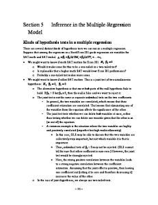
Example: Study weight (y) using age (x1) and height (x2).
100
Data: Age (months), height (inches), weight (pounds) were recorded for a group of school children.
60
60
40
40 120
160
180
200
220
240
50
260
60
70
80
Height
Scatter plots above show that both age and height are linearly related to weight.
Model : y = α + β1 x1 + β 2 x2 + ε with weight y, age x1 , and height x2
Model 1
Model Summary Adjusted R Square .627
4
ANOVAb
SPSS output
R R Square .794a .630
140
Age
3
Model 1
100
80
80
Std. Error of the Estimate 11.868
a. Predictors: (Constant), Height, Age
Coefficient of determination: the percentage of variability in the response variable (Weight) that can be described by predictor variables (Age, Height) through the model.
Regression Residual Total
Sum of Squares 56233.254 32960.761 89194.015
df 2 234 236
Mean Square 28116.627 140.858
F 199.610
Sig. .000a
a. Predictors: (Constant), Height, Age b. Dependent Variable: Weight
Test for significance of the model: p-value = .000 < .05 H0: Model is insignificant (βi’s are all zeros). Ha: Model is significant (Some βi’s are not zeros).
5
6
1
Multiple Regression Model estimation: SPSS output
Coefficientsa
Coefficientsa
Model 1
(Constant) Age Height
Unstandardized Coefficients B Std. Error -127.820 12.099 .240 .055 3.090 .257
Standardi zed Coefficien ts Beta .228 .627
t -10.565 4.360 12.008
Sig. .000 .000 .000
Collinearity Statistics Tolerance VIF .579 .579
1.727 1.727
Model 1
H0: α = 0 vs. Ha: α ≠ 0 p-value = .000 < .05 H0: β1 = 0 vs. Ha: β1 ≠ 0 p-value = .000 < .05 H0: β2 = 0 vs. Ha: β2 ≠ 0 p-value = .000 < .05
.228 .627
t -10.565 4.360 12.008
Collinearity Statistics Tolerance VIF
Sig. .000 .000 .000
.579 .579
1.727 1.727
Least square regression equation:
yˆ = −127 .82 + .24 ⋅ x1 + 3.09 ⋅ x 2
Collinearity* statistics: If the VIF (Variance Inflation Factor) is greater than 10 there is problem of Multicollinearity. (Some said VIF needs to be less than 4.)
The average weight of children 144 months old and whose height is 55 inches would be: −127.82 + .24(144) + 3.09(55) = 76.69 lbs (estimated by the model)
7
8
Other possible models:
How to interpret α , β1 and β 2 ? Model:
Standardi zed Coefficien ts Beta
a. Dependent Variable: Weight
a. Dependent Variable: Weight
Tests for Regression Coefficients
(Constant) Age Height
Unstandardized Coefficients B Std. Error -127.820 12.099 .240 .055 3.090 .257
( y: Weight, x1: Age, x2: Height )
y = α + β1 x1 + β2 x2 + ε
y = α + β 1 x1 + ε y = α + β 2 x2 + ε
where y: Weight, x1: Age, x2: Height
Interaction term
α is the constant or the y-intercept in the model. It is the average response when both predictor variables are 0.
With interaction term (Non-additive): • y = α + β 1 x1 + β 2 x2 + β 3 x1 x2 + ε • y = α + β 1 x1 + β 3 x1 x2 + ε • y = α + β 2 x2 + β 3 x1 x2 + ε
β1 is the rate of change of expected (average) weight per unit change of age adjusted for the height variable.
β2 is the rate of change of expected (average) weight per unit change of height adjusted for the age variable.
9
10
Coefficient Estimation with Interaction Between Age and Height
For boys: Coefficientsa
Model : y = α + β1 x1 + β 2 x2 + β 3 x1 x2 + ε with weight y, age x1 , and height x2 Model 1
Coefficientsa
Model 1
(Constant) Age Height INTAG_HT
Unstandardized Coefficients B Std. Error 66.996 106.189 -.973 .660 -3.13E-02 1.710 1.936E-02 .010
Standardi zed Coefficien ts Beta -.923 -.006 1.636
t .631 -1.476 -.018 1.847
Sig. .529 .141 .985 .066
Collinearity Statistics Tolerance VIF .004 .013 .002
250.009 77.016 501.996
a. Dependent Variable: Weight
• High VIF implies very serious collinearity. • Interaction should not be used in the model.
11
Standardi zed Unstandardized Coefficien Coefficients ts B Std. Error Beta (Constant) -113.713 15.590 Age .308 .084 .289 Height 2.681 .368 .574
t -7.294 3.672 7.283
Sig. .000 .000 .000
Collinearity Statistics Tolerance VIF .443 .443
2.259 2.259
a. Dependent Variable: Weight
• Is there a serious collinearity? • Write the weight prediction equation using age and height as predictor variables. • Find the average weight for boys that are 144 months old and 55 inches tall.
12
2
Multiple Regression
For girls:
Indicator Variables
Coefficientsa
Model 1
(Constant) Age Height
Unstandardized Coefficients B Std. Error -150.597 20.767 .191 .076 3.604 .408
Standardi zed Coefficien ts Beta .186 .650
t -7.252 2.524 8.838
Sig. .000 .013 .000
Collinearity Statistics Tolerance VIF .704 .704
- are binary variables that take only two possible values, 0 and 1, and can be use for including categorical variables in the model.
1.420 1.420
Male: 1 Female: 0
a. Dependent Variable: Weight
• Is there a serious collinearity? • Write the weight prediction equation using age and height as predictor variables. • Find the average weight for boys that are 144 months old and 55 inches tall.
Group Statistics
Weight
Gender Male Female
N
Mean 103.448 98.878
126 111
Std. Deviation 19.968 18.616
Std. Error Mean 1.779 1.767
13
One Binary Independent Variable Model: (A model that models two independent samples situation with equal variances condition.)
14
Two independent samples t-test can be modeled with simple linear regression model SPSS output for two independent samples t-test for comparing the mean weight between male and female. Independent Samples Test
y = α + β1 x1 + ε
Levene's Test for Equality of Variances
where y : Weight, x1: Gender (x1 = 0 for female, x1 = 1 for male)
F Weight
Equal variances assumed Equal variances not assumed
Sig. .630
t-test for Equality of Means
t
.428
df
Sig. (2-tailed)
Mean Difference
Std. Error Difference
L
1.815
235
.071
4.570
2.518
1.823
234.233
.070
4.570
2.507
SPSS output for linear regression with gender as predictor
When x1 = 0: y = α + ε When x1 = 1: y = α + β1 + ε
Coefficientsa
The difference of the means of the two categories is β1. 15
Model 1
(Constant) Gender
Unstandardized Coefficients B Std. Error 98.878 1.836 4.570 2.518
Standardi zed Coefficien ts Beta .118
t 53.846 1.815
Sig. .000 .071
Collinearity Statistics Tolerance VIF 1.000
1.000
16
a. Dependent Variable: Weight
Gender and Age as Predictor Variables Model : y = α + β1 x1 + β 2 x2 + ε
Coefficientsa
with y weight, x1 age, and x2 gender
Model 1
( x2 = 0 female, x2 = 1 male)
(Constant) Age Gender
Unstandardized Coefficients B Std. Error -11.181 8.778 .669 .053 4.539 1.942
Standardi zed Coefficien ts Beta .634 .117
t -1.274 12.705 2.338
Sig. .204 .000 .020
Collinearity Statistics Tolerance VIF 1.000 1.000
1.000 1.000
a. Dependent Variable: Weight
180
160
Age and Gender are both significant variables for predicting weight.
Weight
140
120
100
There is significant difference in average weight between genders if adjusted for age variable.
80
Gender 60
Male
40 120
Female 140
160
180
200
220
240
260
17
18
Age
3
Multiple Regression
Age, Height, & Gender as Predictors 180
Model : y = α + β1 x1 + β 2 x2 + β 3 x3 + ε
160
W e i g h t
with y weight x1 age
140 120 100 80
x2 height
60
x3 gender ( x3 = 0 female, x3 = 1 male)
260240
220 200
180 160
Age
140
50
60
70
80
Gender
Height
Male Female
19
20
Coefficientsa
Model 1
(Constant) Age Height Gender
Unstandardized Coefficients B Std. Error -128.209 12.264 .238 .056 3.105 .267 -.338 1.604
Standardi zed Coefficien ts Beta .226 .630 -.009
t -10.454 4.250 11.621 -.210
Sig. .000 .000 .000 .834
Collinearity Statistics Tolerance VIF .562 .539 .932
1.780 1.854 1.073
a. Dependent Variable: Weight
Gender variable becomes insignificant with Age and Height variables in the model.
How to include a categorical variable in the model? The proper way to include a categorical variable is to use indicator variables. For having a categorical variable with k categories, one should set up k – 1 indicator variables. Example: “Race” variable: White = 1, Black = 2, Hispanic = 3. - 2 indicator variables will be needed.
When comparing the difference in average weights between genders, and adjusted for age and height variables, the difference is statistically insignificant. 21
Common Mistake: Use of the internally coded values of a categorical explanatory variable directly in linear regression modeling calculation. 22
Example:
“Number of hours of exercise per week”
“Race”: White = 1, Black = 2, Hispanic = 3. Use of indicator variables x1 and x2 for Race variable • x1 = 1 represents “White”, otherwise x1 = 0, • x2 = 1 represents “Black”, otherwise x2 = 0, • x1 = 0 and x2 = 0 represents “Hispanic”.
Model:
y = α + β1 x1 + β2 x2 + β3 x3 + ε
“Body Fat Percentage”
“Number of hours of exercise per week”
Model:
y = α + β1 x1 + β2 x2 + β3 x3 + ε
“Race”
Race: White
Interpretation of the model: x1 = 1 and x2 = 0, y = α + β1 + β3 x3 + ε
Race: Black
x1 = 0 and x2 = 1, y = α + β2 + β3 x3 + ε
Race: Hispanic x1 = 0 and x2 = 0, y = α + β3 x3 + ε
“Body Fat Percentage”
“Race”
23
24
4
Multiple Regression
Suppose that the least squares regression equation for the model above is
Example: Study female life expectancy using percentage of urbanization and birth rate.
y = 20 + 2.1 ⋅ x1 + 1.3 ⋅ x2 − .1 ⋅ x3 Estimate the avg. body fat for a white person exercise 10 hours per week: 20 + 2.1 x 1 + 1.3 x 0 – 1.10 = 21.1
Estimate the avg. body fat for a hispanic person exercise 10 hours per week: 20 + 2.1 x 0 + 1.3 x 0 – 1.10 = 18.9
90
80
Female life expectancy 1992
Estimate the avg. body fat for a black person exercise 10 hours per week: 20 + 2.1 x 0 + 1.3 x 1 – 1.10 = 20.2
Female life expectancy 1992
90
70
60
50
40 0
25
10
20
30
40
50
60
80
70
60
50
40 0
20
Births per 1000 population, 1992
Model : y = α + β1 x1 + β 2 x2 + ε Model Summary
R R Square .904a .817
Adjusted R Square .813
60
100 26
80
120
Percent urban, 1992
ANOVAb
y life expectancy, x1 birth rate, x2 percent urbanized Model 1
40
Std. Error of the Estimate 4.89
Model 1
Regression Residual Total
Sum of Squares 12577.056 2825.820 15402.876
df 2 118 120
Mean Square 6288.528 23.948
F 262.595
Sig. .000a
a. Predictors: (Constant), Births per 1000 population, 1992, Percent urban, 1992 b. Dependent Variable: Female life expectancy 1992
a. Predictors: (Constant), Births per 1000 population, 1992, Percent urban, 1992
Test for significance of the model:
p-value = .000 < .05
H0: Model is insignificant (βi’s are all zeros). Ha: Model is significant (Some βi’s are not zeros).
Coefficient of determination: the percentage of variability in the response variable (female life expectancy) that can be described by predictor variables (birth rate, percentage of urbanization) through the model. 27
28
Model estimation: (SPSS output)
Least square regression equation for estimating average response value
Coefficientsa
Model 1
(Constant) Births per 1000 population, 1992 Percent urban, 1992
Unstandardized Coefficients B Std. Error 76.216 2.431
Standardi zed Coefficien ts Beta
t 31.350
Sig. .000
Collinearity Statistics Tolerance VIF
-.555
.045
-.648
-12.196
.000
.551
1.814
.154
.025
.331
6.238
.000
.551
1.814
yˆ = 76 .216 − .555 ⋅ x1 + .154 ⋅ x2
a. Dependent Variable: Female life expectancy 1992
Tests for Regression Coefficients
H0: α = 0 v.s. Ha: α ≠ 0 p-value = .000 < .05 H0: β1 = 0 v.s. Ha: β1 ≠ 0 p-value = .000 < .05 H0: β2 = 0 v.s. Ha: β2 ≠ 0 p-value = .000 < .05
Collinearity*statistics:If the VIF (Variance Inflation Factor) is greater than 10 there is multicollinearity problem. (Some said VIF needs to be less than 4.) 29
The average female life expectancy for the countries whose birth rate per 1000 is 30 and whose percentage of urbanization is 40 would be 76.216 - 0.555(30) + 0.154(40) = 65.726. 30
5
Multiple Regression
Construction of regression models
Use of regression analysis • Description (model, system, relation): Relation between life expectancy & birth rate, GDP, … Relation between salary & rank, years of service, …
• Control: Died too young, underpaid, overpaid, …
• Prediction: Life expectancy, salary for new comers, future salary, …
• Variable screening (important factors):
1. Hypothesize the form of the model for μ y| x1, x2 , x3 ,..., xq – Selecting predictor variables. – Deciding functional form of the regression equation. – Defining scope of the model (design range). 2. Collect the sample data (observations, experiments). 3. Use sample estimate unknown parameters in the model. 4. Understand the distribution of the random error. 5. Model diagnostics, residual analysis. 6. Apply the model in decision making. 7. Review the model with new data.
Significant factors for life expectancy, Significant factors for salary. 31
32
6