1

Prof. Òscar Jordà

Problem Set 4

Due Date: Thursday, May 22

ECONOMETRICS STUDENT’S NAME: Multiple Choice Questions [20 pts] Please provide your answers to this section below: 1.

6.

2.

7.

3.

8.

4.

9.

5.

10.

1)

In the multiple regression model, the adjusted R2, R 2 a. b. c. d.

cannot be negative. will never be greater than the regression R2. equals the square of the correlation coefficient r. cannot decrease when an additional explanatory variable is added.

Answer: b

2)

Under imperfect multicollinearity e. f. g. h.

the OLS estimator cannot be computed. two or more of the regressors are highly correlated. the OLS estimator is biased even in samples of n > 100. the error terms are highly, but not perfectly, correlated.

Answer: b

3)

The following linear hypothesis can be tested using the F-test with the exception of a. β 2 = 1 and β 3 = β 4 / β 5 . b. β 2 = 0 . c. β1 + β 2 = 1 and β 3 = −2 β 4 . d. β0 = β1 and β1 = 0.

2 Answer: a

4)

When there are omitted variables in the regression, which are determinants of the dependent variable, then a. you cannot measure the effect of the omitted variable, but the estimator of your included variable(s) is (are) unaffected. b. this has no effect on the estimator of your included variable because the other variable is not included. c. this will always bias the OLS estimator of the included variable. d. the OLS estimator is biased if the omitted variable is correlated with the included variable. Answer: d

5)

Imagine you regressed earnings of individuals on a constant, a binary variable (“Male”) which takes on the value 1 for males and is 0 otherwise, and another binary variable (“Female”) which takes on the value 1 for females and is 0 otherwise. Because females typically earn less than males, you would expect a. the coefficient for Male to have a positive sign, and for Female a negative sign. b. both coefficients to be the same distance from the constant, one above and the other below. c. none of the OLS estimators to exist because there is perfect multicollinearity. d. this to yield a difference in means statistic. Answer: c

6)

If you had a two regressor regression model, then omitting one variable which is relevant a. will have no effect on the coefficient of the included variable if the correlation between the excluded and the included variable is negative. b. will always bias the coefficient of the included variable upwards. c. can result in a negative value for the coefficient of the included variable, even though the coefficient will have a significant positive effect on Y if the omitted variable were included. d. makes the sum of the product between the included variable and the residuals different from 0. Answer: c

7)

To test joint linear hypotheses in the multiple regression model, you need to a. compare the sums of squared residuals from the restricted and unrestricted

3

model. b. use the heteroskedasticity-robust F-statistic. c. use several t-statistics and perform tests using the standard normal distribution. d. compare the adjusted R2 for the model which imposes the restrictions, and the unrestricted model. Answer: b

8) Under the least squares assumptions for the multiple regression problem (zero conditional mean for the error term, all Xi and Yi being i.i.d., all Xi and ui having finite fourth moments, no perfect multicollinearity), the OLS estimators for the slopes and intercept a. have an exact normal distribution for n > 25. b. are BLUE. c. have a normal distribution in small samples as long as the errors are homoskedastic. d. are unbiased and consistent. Answer: d

9) If you reject a joint null hypothesis using the F-test in a multiple hypothesis setting, then a. b. c. d.

a series of t-tests may or may not give you the same conclusion. the regression is always significant. all of the hypotheses are always simultaneously rejected. the F-statistic must be negative.

Answer: a

10) When your multiple regression function includes a single omitted variable regressor, then a. use a two-sided alternative hypothesis to check the influence of all included variables. b. the estimator for your included regressors will be biased if at least one of the included variables is correlated with the omitted variable. c. the estimator for your included regressors will always be biased. d. lower the critical value to 1.645 from 1.96 in a two-sided alternative hypothesis to test the significance of the coefficients of the included variables. Answer: b

4

Problems [40 pts] Instructions: The goal of the problem set is to understand what you are doing rather than just getting the correct result. Please show your work clearly and neatly. Please write your answers in the space provided. 1) The cost of attending your college has once again gone up. Although you have been told that education is investment in human capital, which carries a return of roughly 10% a year, you (and your parents) are not pleased. One of the administrators at your university/college does not make the situation better by telling you that you pay more because the reputation of your institution is better than that of others. To investigate this hypothesis, you collect data randomly for 100 national universities and liberal arts colleges from the 2000-2001 U.S. News and World Report annual rankings. Next you perform the following regression

Cost = 7,311.17 + 3,985.20 × Reputation – 0.20 × Size (2,058.63) (664.58)

(0.13)

+ 8,406.79 × Dpriv – 416.38 × Dlibart – 2,376.51 × Dreligion (2,154.85) (1,121.92) (1,007.86) R2=0.72, SER = 3,773.35 where Cost is Tuition, Fees, Room and Board in dollars, Reputation is the index used in U.S. News and World Report (based on a survey of university presidents and chief academic officers), which ranges from 1 (“marginal”) to 5 (“distinguished”), Size is the number of undergraduate students, and Dpriv, Dlibart, and Dreligion are binary variables indicating whether the institution is private, a liberal arts college, and has a religious affiliation. The numbers in parentheses are heteroskedasticity-robust standard errors. (a)

Interpret the results and indicate whether or not the coefficients are significantly different from zero. Do the coefficients have the expected sign? Answer: An increase in reputation by one category, increases the cost by roughly $3,985. The larger the size of the college/university, the lower the cost. An increase of 10,000 students results in a $2,000 lower cost. Private schools charge roughly $8,406 more than public schools. A school with a religious affiliation is approximately $2,376 cheaper, presumably due to subsidies, and a liberal arts college also charges roughly $416 less. There are no observations close to the origin, so there is no direct interpretation of the intercept. Other than perhaps the coefficient on liberal arts colleges, all coefficients have the expected sign, although that coefficient is not significantly different from zero. All other coefficients are statistically significant at conventional levels, with the exception of the size coefficient, which carries a t-statistic of 1.54, and hence is not statistically significant at the 5% level (using a one-sided alternative hypothesis).

(b)

What is the forecasted cost for a liberal arts college, which has no religious affiliation, a size of 1,500 students and a reputation level of 4.5? (All liberal arts colleges are private.) Answer: $ 32,935.

5 (c)

To save money, you are willing to switch from a private university to a public university, which has a ranking of 0.5 less and 10,000 more students. What is the effect on your cost? Is it substantial? Answer: Roughly $ 12,4.00. Since over the four years of education, this implies approximately $50,000, it is a substantial amount of money for the average household.

(d)

What is the p-value for the null hypothesis that the coefficient on Size is equal to zero? Based on this, should you eliminate the variable from the regression? Why or why not? Answer: Using a one-sided alternative hypothesis, the p-value is 6.2 percent. Variables should not be eliminated simply on grounds of a statistical test. The sign of the coefficient is as expected, and its magnitude makes it important. It is best to leave the variable in the regression and let the reader decide whether or not this is convincing evidence that the size of the university matters.

(e)

You want to test simultaneously the hypotheses that

β size = 0 and β Dlibart = 0 . Your regression

package returns the F-statistic of 1.23. Can you reject the null hypothesis? Answer: The critical value for F2,∞ is 3.00 (5% level) and 4.61 (1% level). Hence you cannot reject the null hypothesis in this case. (f)

Eliminating the Size and Dlibart variables from your regression, the estimation regression becomes

Cost = 5,450.35 + 3,538.84 × Reputation + 10,935.70 × Dpriv – 2,783.31 × Dreligion; (1,772.35) (590.49)

(875.51)

(1,180.57)

R2=0.72, SER = 3,792.68 Why do you think that the effect of attending a private institution has increased now? Answer: Private institutions are smaller, on average, and some of these are liberal arts colleges. Both of these variables had negative coefficients. (g)

You give a final attempt to bring the effect of Size back into the equation by forcing the assumption of homoskedasticity onto your estimation. The results are as follows:

Cost = 7,311.17 + 3,985.20 × Reputation – 0.20 × Size (1,985.17) (593.65)

(0.07)

+ 8,406.79 × Dpriv – 416.38 × Dlibart – 2,376.51 × Dreligion (1,423.59) (1,096.49) (989.23) R2=0.72, SER = 3,682.02 Calculate the t-statistic on the Size coefficient and perform the hypothesis test that its coefficient is zero. Is this test reliable? Explain. Answer: Although the coefficient would be statistically significant in this case, the test is unreliable and should not be used for statistical inference. There is no theoretical suggestion here that the errors might be homoskedastic. Since the standard errors are

6 quite different here, you should use the more reliable ones, i.e. the heteroskedasticityrobust. (h)

What can you say about causation in the above relationship? Is it possible that Cost affects Reputation rather than the other way around? Answer: It is very possible that the university president and chief academic officer are influenced by the cost variable in answering the U.S. News and World Report survey. If this were the case, then the above equation suffers from simultaneous causality bias, a topic that will be covered in a later chapter. However, this poses a serious threat to the internal validity of the study.

2) You have collected data for 104 countries to address the difficult questions of the determinants for differences in the standard of living among the countries of the world. You recall from your macroeconomics lectures that the neoclassical growth model suggests that output per worker (per capita income) levels are determined by, among others, the saving rate and population growth rate. To test the predictions of this growth model, you run the following regression:

RelPersInc = 0.339 – 12.894 × n + 1.397 × sK , R2=0.621, SER = 0.177 (0.068) (3.177)

(0.229)

where RelPersInc is GDP per worker relative to the United States, n is the average population growth rate, 1980-1990, and sK is the average investment share of GDP from 1960 to1990 (remember investment equals saving). Numbers in parentheses are for heteroskedasticity-robust standard errors. (a)

Interpret the results. Do the signs correspond to what you expected them to be? Explain. Answer: The Solow growth model predicts higher productivity with higher saving rates and lower population growth. The signs therefore correspond to prior expectations. A 10 percent point increase in the saving rate results in a roughly 14 percent increase in per capita income relative to the United States. Lowering the population growth rate by 1 percent results in a 13 percent higher per capita income relative to the United States. It is best not to interpret the intercept. The regression explains approximately 62 percent of the variation in per capita income among the 104 countries of the world.

(b)

Calculate the t-statistics and test whether or not each of the population parameters are significantly different from zero. Answer: The t-statistics for population growth and the saving rate are –4.06 and 6.10, making both coefficients significantly different from zero at conventional levels of significance.

(c)

The overall F-statistic for the regression is 79.11. What is the critical value at the 5% and 1% level? What is your decision on the null hypothesis? Answer: The critical value is 3.00 and 4.61 respectively, allowing you to reject the null hypothesis that all slope coefficients are zero.

(d)

You remember that human capital in addition to physical capital also plays a role in determining the standard of living of a country. You therefore collect additional data on the average educational attainment in years for 1985, and add this variable (Educ) to the above regression. This results in the modified regression output:

7

RelPersInc = 0.046 – 5.869 × n + 0.738 × sK + 0.055 × Educ, R2=0.775, SER = 0.1377 (0.079) (2.238)

(0.294)

(0.010)

How has the inclusion of Educ affected your previous results? Answer: The coefficient on the population growth rate is roughly half of what it was originally, while the coefficient on the saving rate has approximately doubled. The regression R2 has increased significantly. (e)

Upon checking the regression output, you realize that there are only 86 observations, since data for Educ is not available for all 104 countries in your sample. Do you have to modify some of your statements in (d)? Answer: When comparing results, you should ensure that the sample is identical, since comparisons are not valid otherwise. In addition, there are now less than 100 observations, making inference based on the standard normal distribution problematic.

(f)

Brazil has the following values in your sample: RelPersInc = 0.30, n = 0.021, sK = 0.169, Educ = 3.5. Does your equation overpredict or underpredict the relative GDP per worker? What would happen to this result if Brazil managed to double the average educational attainment? Answer: The predicted value for Brazil is 0.240. Hence the regression underpredicts Brazil’s per capita income. Increasing Educ to 7.0 would result in a predicted per capita income of 0.43, which is a substantial increase from both its current actual position and the previously predicted value.

3)

(Requires Appendix Material) The rule-of-thumb F-statistic is given by the formula

F=

( SSRrestricted − SSRunrestricted ) / q SSRunrestricted /( n − k unrestricted − 1)

where SSRrestricted is the sum of squared residuals from the restricted regression, SSRunrestricted is the sum of squared residuals from the unrestricted regression, q is the number of restrictions under the null hypothesis, and kunrestricted is the number of regressors in the unrestricted regression. Prove that this formula is the same as the following formula based on the regression R2 of the restricted and unrestricted regression:

F= Answer: Since R = 1 − 2

2 2 ( Runrestrict ed − Rrestricted ) / q 2 (1 − Runrestrict ed ) /( n − k unrestricted − 1)

SSR , SSR = TSS (1 − R 2 ) . Substitution into the first equation then TSS

results in the second equation, once the “1” in the numerator is canceled, and the TSS is factored out in the numerator.

8

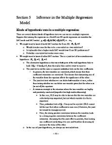
EViews Exercise [40 pts] Part 1 TESTSCR vs. MEAL_PCT

TESTSCR vs. EL_PCT 720

720

700

700

680 TESTSCR

TESTSCR

680 660 640

660 640 620

620

600

600 0

10

20

30

40

50

60

70

80

0

90

20

40

60

80

MEAL_PCT

EL_PCT

TESTSCR vs. CALW _PCT 720 700

TESTSCR

680

TESTSCR EL_PCT MEAL_PCT CALW _PCT

660 640 620 600 580 0

10

20

30

40

50

60

70

80

CALW _PCT

Part 2 Dependent Variable: TESTSCR Method: Least Squares Date: 05/14/03 Time: 15:21 Sample: 1 420 Included observations: 420 White Heteroskedasticity-Consistent Standard Errors & Covariance Variable

Coefficient

Std. Error

t-Statistic

Prob.

C STR

698.9330 -2.279808

10.36436 0.519489

67.43619 -4.388557

0.0000 0.0000

R-squared Adjusted R-squared S.E. of regression Sum squared resid Log likelihood Durbin-Watson stat

0.051240 0.048970 18.58097 144315.5 -1822.250 0.129062

Mean dependent var S.D. dependent var Akaike info criterion Schwarz criterion F-statistic Prob(F-statistic)

654.1565 19.05335 8.686903 8.706143 22.57511 0.000003

TESTSCR 1.000000 -0.644124 -0.868772 -0.626853

100

9

Dependent Variable: TESTSCR Method: Least Squares Date: 05/14/03 Time: 15:23 Sample: 1 420 Included observations: 420 White Heteroskedasticity-Consistent Standard Errors & Covariance Variable

Coefficient

Std. Error

t-Statistic

Prob.

C STR EL_PCT

686.0322 -1.101296 -0.649777

8.728224 0.432847 0.031032

78.59930 -2.544307 -20.93909

0.0000 0.0113 0.0000

R-squared Adjusted R-squared S.E. of regression Sum squared resid Log likelihood Durbin-Watson stat

0.426431 0.423680 14.46448 87245.29 -1716.561 0.685575

Mean dependent var S.D. dependent var Akaike info criterion Schwarz criterion F-statistic Prob(F-statistic)

654.1565 19.05335 8.188387 8.217246 155.0136 0.000000

Dependent Variable: TESTSCR Method: Least Squares Date: 05/14/03 Time: 15:24 Sample: 1 420 Included observations: 420 White Heteroskedasticity-Consistent Standard Errors & Covariance Variable

Coefficient

Std. Error

t-Statistic

Prob.

C STR EL_PCT MEAL_PCT

700.1500 -0.998309 -0.121573 -0.547346

5.568450 0.270080 0.032832 0.024107

125.7352 -3.696348 -3.702926 -22.70460

0.0000 0.0002 0.0002 0.0000

R-squared Adjusted R-squared S.E. of regression Sum squared resid Log likelihood Durbin-Watson stat

0.774516 0.772890 9.080079 34298.30 -1520.499 1.437595

Mean dependent var S.D. dependent var Akaike info criterion Schwarz criterion F-statistic Prob(F-statistic)

654.1565 19.05335 7.259521 7.298000 476.3064 0.000000

Dependent Variable: TESTSCR Method: Least Squares Date: 05/14/03 Time: 15:27 Sample: 1 420 Included observations: 420 White Heteroskedasticity-Consistent Standard Errors & Covariance Variable

Coefficient

Std. Error

t-Statistic

Prob.

C STR EL_PCT CALW_PCT

697.9987 -1.307984 -0.487620 -0.789965

6.920369 0.339076 0.029582 0.067660

100.8615 -3.857494 -16.48352 -11.67557

0.0000 0.0001 0.0000 0.0000

R-squared Adjusted R-squared S.E. of regression Sum squared resid Log likelihood

0.628543 0.625864 11.65429 56502.17 -1625.328

Mean dependent var S.D. dependent var Akaike info criterion Schwarz criterion F-statistic

654.1565 19.05335 7.758704 7.797183 234.6381

10 Durbin-Watson stat

1.094470

Prob(F-statistic)

0.000000

Dependent Variable: TESTSCR Method: Least Squares Date: 05/14/03 Time: 15:26 Sample: 1 420 Included observations: 420 White Heteroskedasticity-Consistent Standard Errors & Covariance Variable

Coefficient

Std. Error

t-Statistic

Prob.

C STR EL_PCT MEAL_PCT CALW_PCT

700.3918 -1.014353 -0.129822 -0.528619 -0.047854

5.537418 0.268861 0.036258 0.038117 0.058654

126.4835 -3.772775 -3.580509 -13.86844 -0.815863

0.0000 0.0002 0.0004 0.0000 0.4150

R-squared Adjusted R-squared S.E. of regression Sum squared resid Log likelihood Durbin-Watson stat

0.774850 0.772680 9.084273 34247.46 -1520.188 1.429595

Mean dependent var S.D. dependent var Akaike info criterion Schwarz criterion F-statistic Prob(F-statistic)

654.1565 19.05335 7.262800 7.310898 357.0541 0.000000

Part 3 Dependent Variable: TESTSCR_STD Method: Least Squares Date: 05/14/03 Time: 15:47 Sample: 1 420 Included observations: 420 White Heteroskedasticity-Consistent Standard Errors & Covariance Variable

Coefficient

Std. Error

t-Statistic

Prob.

C STR

2.350057 -0.119654

0.543965 0.027265

4.320233 -4.388557

0.0000 0.0000

R-squared Adjusted R-squared S.E. of regression Sum squared resid Log likelihood Durbin-Watson stat

0.051240 0.048970 0.975207 397.5303 -584.4076 0.129062

Mean dependent var S.D. dependent var Akaike info criterion Schwarz criterion F-statistic Prob(F-statistic)

2.52E-06 1.000000 2.792417 2.811657 22.57511 0.000003

Dependent Variable: TESTSCR_STD Method: Least Squares Date: 05/14/03 Time: 15:47 Sample: 1 420 Included observations: 420 White Heteroskedasticity-Consistent Standard Errors & Covariance Variable

Coefficient

Std. Error

t-Statistic

Prob.

C STR EL_PCT

1.672973 -0.057801 -0.034103

0.458094 0.022718 0.001629

3.652032 -2.544307 -20.93909

0.0003 0.0113 0.0000

R-squared

0.426431

Mean dependent var

2.52E-06

11 Adjusted R-squared S.E. of regression Sum squared resid Log likelihood Durbin-Watson stat

0.423680 0.759157 240.3252 -478.7192 0.685575

S.D. dependent var Akaike info criterion Schwarz criterion F-statistic Prob(F-statistic)

1.000000 2.293901 2.322760 155.0136 0.000000

Dependent Variable: TESTSCR_STD Method: Least Squares Date: 05/14/03 Time: 15:46 Sample: 1 420 Included observations: 420 White Heteroskedasticity-Consistent Standard Errors & Covariance Variable

Coefficient

Std. Error

t-Statistic

Prob.

C STR EL_PCT MEAL_PCT

2.413931 -0.052395 -0.006381 -0.028727

0.292256 0.014175 0.001723 0.001265

8.259654 -3.696348 -3.702926 -22.70460

0.0000 0.0002 0.0002 0.0000

R-squared Adjusted R-squared S.E. of regression Sum squared resid Log likelihood Durbin-Watson stat

0.774516 0.772890 0.476561 94.47783 -282.6574 1.437595

Mean dependent var S.D. dependent var Akaike info criterion Schwarz criterion F-statistic Prob(F-statistic)

2.52E-06 1.000000 1.365035 1.403514 476.3064 0.000000

Dependent Variable: TESTSCR_STD Method: Least Squares Date: 05/14/03 Time: 15:46 Sample: 1 420 Included observations: 420 White Heteroskedasticity-Consistent Standard Errors & Covariance Variable

Coefficient

Std. Error

t-Statistic

Prob.

C STR EL_PCT CALW_PCT

2.301023 -0.068649 -0.025592 -0.041461

0.363210 0.017796 0.001553 0.003551

6.335239 -3.857494 -16.48352 -11.67557

0.0000 0.0001 0.0000 0.0000

R-squared Adjusted R-squared S.E. of regression Sum squared resid Log likelihood Durbin-Watson stat

0.628543 0.625864 0.611666 155.6404 -387.4859 1.094470

Mean dependent var S.D. dependent var Akaike info criterion Schwarz criterion F-statistic Prob(F-statistic)

2.52E-06 1.000000 1.864219 1.902697 234.6381 0.000000

Dependent Variable: TESTSCR_STD Method: Least Squares Date: 05/14/03 Time: 15:44 Sample: 1 420 Included observations: 420 White Heteroskedasticity-Consistent Standard Errors & Covariance Variable

Coefficient

Std. Error

t-Statistic

Prob.

12 C STR EL_PCT MEAL_PCT CALW_PCT R-squared Adjusted R-squared S.E. of regression Sum squared resid Log likelihood Durbin-Watson stat

2.426625 -0.053238 -0.006814 -0.027744 -0.002512 0.774850 0.772680 0.476781 94.33779 -282.3459 1.429595

0.290627 0.014111 0.001903 0.002001 0.003078

8.349621 -3.772775 -3.580509 -13.86844 -0.815863

Mean dependent var S.D. dependent var Akaike info criterion Schwarz criterion F-statistic Prob(F-statistic)

0.0000 0.0002 0.0004 0.0000 0.4150 2.52E-06 1.000000 1.368314 1.416412 357.0541 0.000000

The coefficients from these regressions show, for a one unit increase in the regressor, how many standard deviations away from the mean will the test score vary.

Part 4 (a) Specification 3. The adjusted R-square increases when we add percent of English learners and percent eligible for subsidized lunch as independent variables. Addition of percent of public income assistance variable does not increase the explanatory power of the regression. Also, the coefficient on this variable is insignificant. These results are the same originally obtained since the transformation of the dependent variable is such that is does not affect the fit of the model. (b) Here is the Eviews output Wald Test: Equation: Untitled Test Statistic F-statistic Chi-square

Value 0.388461 0.776922

df Probability (2, 415) 2

0.6783 0.6781

Value

Std. Err.

0.002251 -0.002512

0.014142 0.003078

Null Hypothesis Summary: Normalized Restriction (= 0) C(2) - 2*C(4) C(5)

The p-value for F-statistics is 0.6783, hence we fail to reject the null hypothesis. (c) The book offers a good way to check this answer against your interpretation of the results.