Monocular Simultaneous Localization and Mapping using Color Features Jason P. Moran, Member, Mechanical Engineering ‘11
Abstract—SLAM (Simultaneous Localization and Mapping) is on the forefront of today's robotic research. Over the past 10 years a variety of SLAM "solutions" have been discussed in academia. One of the earlier methods of SLAM involved using artificial landmarks to help make the feature extraction aspect of SLAM more manageable. While there are more complex SLAM solutions available, this implementation is unique in its method of feature extraction. Since the intensity of colors change drastically, the robot uses a trained multinomial logistic function (supervised learning) to classify image pixels. A version k-means clustering (unsupervised learning) was implemented using a novel approach for determining cluster quantities and centers to ultimately find landmarks. Monocular SLAM is a more difficult problem than LIDAR SLAM in that features provide bearing only data. Furthermore, a reasonable estimate of a landmarks location from one image is not possible. A method for adding landmarks to map was developed as well as associating landmarks in the current image to those already in the map. Lastly, an Extended Kalman Filter was implemented to fuse 2D odometry data with measurement updates.
I. INTRODUCTION
I
magine a robot that is sitting in a completely known environment. Localizing oneself within the environment becomes a fairly simple task (one could simply use Markov localization). Conversely, imagine a robot that knew its location perfectly in an unknown environment. Developing a map would be as simple filling an occupancy grid from laser range finder data. But what if the robot knows neither its location nor the environment? This is the domain of Simultaneous Localization and Mapping (SLAM), sometimes also called Concurrent Mapping and Localization (CML). SLAM is "one of the most fundamental problems in robotics." [1] The problem is difficult because creating a map depends on localization and vice versa. One of the first full comprehensive solutions to SLAM is presented in Dissanayake et al. A Solution to the Simultaneous Map Building (SLAM) Problem paper [2]. The paper describes a potential estimation-theoretic Kalman filter approach for providing a solution to the full SLAM problem (paper proves what was shown in SLAM lecture). Since this paper, many more "solutions" to SLAM problem have come about (ie. Extended Kalman Filters, Unscented Kalman Filters, and so on). One of the difficult aspects of SLAM, which the paper does not go into depth on, is landmark selection. To solve the SLAM problem, one must choose features of interest (landmarks) and then use these to localize and map.
Proper selection of landmarks in a map is one topic in the forefront of research today. The project described below assumes no knowledge of landmarks other than a color (red, pink, orange, yellow, purple, green). This is different from the midterm project which assumed landmark location was also known. All the code required for the SLAM solution was written personally by the solitary author. This includes but is not limited too, UDP communicator wrapper, K-means clustering algorithm, multinomial logistic pixel classifier, full implementation of EKF, data association, map management, camera model, and transformation functions. There is a short video which was submitted as well for demo day. There is more video that can be submitted that shows more errors in the algorithm if is needed. A copy of the authors k-means clustering implementation will also be attached. The only program that was not written by the author was SMLR, which was used to calculate the weights for the multinomial logistic function. Other than that, no special MATLAB code was used other than plot commands, and inverse matrix commands, so the code can easily be ported to any other language with proper changing of syntax and indices. II. BACKGROUND The past 10 years has seen extensive research on SLAM methods. Numerous survey papers have been written, but one (name) was done specifically on bearing-only SLAM [3]. Various techniques for bearing-only SLAM exist, including particle filter SLAM [4][5] and the most frequent EKF SLAM [3]. Different methods for landmark initialization include standard Gaussian initialization as in [6], depth paramaterization [7] and initialization through sum of Gaussians to approximate a uniform distribution (GSF)[8]. Furthermore many different feature extractors have been used including lines as in [6], corners [9], sift features, and color as in [10], III. ROBOT A. Hardware The platform being used is the Pioneer P3-DX robot made by MobileRobots. The robot has an onboard mini-ITX computer as a Hokuyo LIDAR unit and a camera with 38 degrees field view. The robot has two rear wheels, each controlled by an independent motor. In the front there is a single caster. The mechanical design of the robot allows it to be accurately modeled as a 3 DOF (x,y,theta) system in 2D. Because of the front caster and independent wheels the DOFs can be successfully decoupled (ASL Wiki).
Currently, the mini-ITX computer runs Linux and has an ORCA framework installed for communicating with the robot. The ORCA framework is difficult to create components in so the robot will be run using a UDP communicator in MATLAB. Using the UDP communicator limits the speed of the measurement update since only about 9 frames per second can be sent through the communicator. Furthermore the resolution of these frames must be reduced using a standard jpeg compression format from 640 x 480 to 320 x 240 to allow high enough fps for a successful SLAM solution. The fire wire camera being used has a maximum focal length of 4.3mm (optimal focus is about 2mm), a pixel size of 5.6um, and 2.5 key frames per second.
Eq. 1 Since the camera is not at the center of the robot the camera coordinate system would need to be transformed into the robot coordinate system. It is easiest to perform this transformation post measurement and data association. The final, and most important aspect is how a potential landmark appears relative to the robot in a global reference frame. This ultimately determines the measurement equation that will be used, along with its Jacobian, in the extended Kalman filter.
Feature θ
y
φ Robot x B. Robot Model As described above, the robot can be modeled using standard (x,y,φ) state space. There are a few necessary transformations that must be made to put the measurement into the same coordinate system as odometry. First, the odometry center must be transformed from its position at the center of the wheels to the center of the rover. This can be accomplished with a simple rotation matrix, and translation can be ignored since the state space model does not include a third dimension. The next aspect to consider is the transformation from a point in an image to a position relative to the robot camera to determine a bearing. This bearing can be determined using a simple pinhole camera model. Fig 2. details this camera model. Here, f is focal length, u0 is the principal point (typically the center of the image), and u is a pixel location.
Fig 3. Robot in global reference frame. Fig 3. above depicts the robot in its global coordinate frame. Here the coordinate of the robot are (x,y,φ) and the coordinates of the feature can be represented by (xL, yL). The resulting measurement equation and its Jacobian components are. Eq. 2 Eq. 3 Eq. 4 Eq. 5
Landmark Where Eq. 6 θ
IV. METHODS
Image
f u0
Fig.2 Camera Model
u
A. General Flow The SLAM algorithm has many necessary components, each of which are an area of research in computer science. The following flowchart (Fig 4.) depicts interconnectedness of all the SLAM components.
Feature Extraction
Camera
Odometry
specific color. Only pixels with a probability of greater that 75% were accepted.
Time Update
Data Association
Map Management
Measurement Update
Fig. 5 Original Image at resolution 320 x 240 Figure 4. Flow Chart B. Feature Extraction The features being used are colored cones and tubes, with hope that these can be extended to lamp posts, telephone posts, and trees. The objects have cylindrical cross sections so that their center will be the same viewed from any angle, the producing an extremely stable feature. The first attempt at producing color segmentation feature extraction produced unreliable and sparse data. First a median filter was applied to remove random noise and incorrect color mapping by the CCD. Sample RGB values were taken for each landmark, and statistics of the data were computed. Pixels were classified if they and their neighbors fell within a specified amount of standard deviations from the mean for each color channel. This method proved unreliable since the cameras exposure and thus intensity change greatly, especially when the robot was moving. Recalculating statistics for a wide range of intensities resulted in large standard deviations and falsely classified many pixels. An attempt was then made to move to a color mapping that was independent of intensity. RG chromaticity was used (Ratio of colors to the total image intensity). This worked better, but required a large amount of hand tuning. To avoid tuning frustration, supervised learning was employed. Not only did it get rid of tuning but it also classified pixels much more accurately. A Multinomial Logistic Function was used to classify pixels and create a segmented image for each color. Weights were created by using a training set of 7 classes (6 different colors and one other category). The training set was taken over a wide range of image intensities and both with the robot moving and without. Each class had 200 data points and weights were obtained using SMLR, a java program from Duke University. The state vector for the equation was the three RGB values. This yields 4 weights, one for each value and an offset. Using the weights obtained from the program, the equation (number) gives the probability that a pixel is a
Fig 6. Segmentation of color pink
Fig 7. Segmentation of color orange With the segmented images it was necessary to find the number of objects, identified by white pixels. One method would be to implement a blob filter. This method was initially employed. Blobs were initially kept if they were greater than a certain size. This method would often produce too many blobs because a landmark may be represented by a sparse segmentation. If landmarks had words, were partially occluded, or patches of another color, it was important that they still be classified as one landmark.
Unsupervised learning was then performed on each of the segmented images. An implementation of k-means clustering was personally written, and a novel method for choosing cluster centers and guesses was created. The method entailed searching columns and rows for white pixels. If the pixels were close to other pixels they would be considered one cluster. The k-means clustering algorithm written was sensitive to guesses for cluster centers. Originally simple elbow method program was written to choose k. This program chose k accurately sometimes but did provide proper guesses for cluster centers. Improper guesses as to cluster numbers and centers would result in creating inexistent features or determining feature centers unreliably. The feature extraction algorithm is independent of feature size and shape (features with circular cross sections only necessary for stability) and the object does not need to be a uniform color, and can have writing, tape marks, holes, etc. It was designed this way so it could be extended easily to other objects easily.
associations and has a few bad measurement updates, pose will be miss calculated and all future data associations are likely to be incorrect. D. Map Management Map management is another aspect of importance. Features in the map must be reliable as they are ultimately use in the measurement update of the EKF. If inexistent features find their way into the map it can ruin data association. Furthermore if features are too densely packed, have variances that are too large, or are sparse, it can cause serious problems. To deal with this, a temporary map was created along with a set of map management rules. The rules were decided independently by the author. Essentially, the rules are as follows:
1) If a detected feature is associated with a map feature, the feature's variance is updated if the robots state variance is below a threshold. The feature measurement will then be used for a measurement update. 2) If the feature does not associate with a map feature, the temporary map is checked for possible associations. 3) If there is a positive association with the temporary map, the feature's variance is updated regardless of state variance.
Fig. 8 Shows center identification. Extractor even pulls out the small pink beacon far away.
4) The map is checked for features with variances that are too high. These features are moved to the temporary map. 5) The temporary map is checked for features with low variance, and these features are moved to the map. 6) The temporary map is pruned. Features with very large variances are permanently removed to avoid poor data association with the temporary map. 7) Features that were in neither map were added to a temporary map.
Fig. 9 Shows center estimate for orange cone. Notice detection does not depend on shape. C. Data Association Using the state from after the time update, an expected angle in image is calculated for all features in the map. Features found in the current image are compared with map features of the same color and a chi-squared hypothesis test is used to determine if features are a match. The test takes into account the positional variance of the robot as well as the variance of the feature, it is described in equation which was derived from [6] Data association in this implementation of SLAM is extremely dependent on prior pose estimate. If the robot makes a few bad data
The last part of map management is feature initialization. Various papers have been written on the subject but ultimately there was not enough time to investigate the subject fully. The method that was chosen stems from [6] as well as the equations in the landmark initialization section of that paper. Landmarks that have never been seen before are initialized to be a Gaussian distribution largest in the depth direction. The variance in the depth direction is initially set to be the length of the room while the variance perpendicular to depth is dependent on angular variance, which is a function of camera resolution.
Fig 10. Landmark first initialized to a large Gaussian. Than after combining multiple Gaussians at different angles, a low variance is obtained and a strong estimate of feature location is obtained. E. Extended Kalman Filter The last aspect of the SLAM is the filter which merges measurement data with time data. Two models were considered for the time update. One was the velocity model which uses, vehicle velocities as a method for time update. The other method, which was ultimately chosen, is the odometry driven model described in Thrun's Probabilistic Robotics. The measurement update can then be easily obtained with the measurement Jacobian in equations 3-5 and the variance of the landmark. V. RESULTS The components described above for were combined and run on the pioneer in the ASL lab. Odometry Time updates occurred at a rate of 30 hz, while measurement updates could only take place at 5hz. This low measurement update rate can be partially attributed to the low frame rate transmission rate of the camera. Each frame at 320 x 240 took roughly a eighth of a second to transmit. Then processing (including segmentation, k-means, and data association) was clocked to be an average .146 seconds. As a result, an image was not always available after image processing and measurement update had been complete. The feature extractor built was extremely successful at detecting landmarks. The image classifier (multinomial logistic classifier) when tested on a different data set of equal size achieved a 98.28% success rate with most miss classifications coming between red and pink as well as green and background. The segmentation used a high probability threshold for successful classification. This high threshold result in only 90% being classified correctly, with a vast majority of miss classifications being to background (thus black in segmentation). The next part of the feature extractor was the k-means clustering algorithm and the novel choose k algorithm. These two algorithms, correctly identified all landmarks 91% of the time. Most miss classification occurred when landmarks of the same color were too close together, the landmark had sufficient glare, or was sufficiently far away. The overall result is that the algorithm was capable of detecting landmarks 84% of the time (data set of 100). A majority of failed cases were a landmark was not identified at all. This lack of identification is the best scenario as it
does not mess with feature variances in data association or map management. Finally, the robot was capable of doing SLAM but only minimally. A difficult aspect that occurred was initializing new landmarks. Since, the camera field of view was only 42.25 degrees, landmarks could not be initialized with simply one pass. As a result the robot would have to drive around the landmark continuously looking for the feature. After this length path and turning, a few features could be initialized, but this is only after odometry was running for a sufficient period of time, thus the uncertainty of the physical robot was high by the time the features could be initialized. As a result careful placement of the features was needed, and fine tuning of the map management system was needed. One way this could be improved, and many authors have done this, is to use either a wide angle lense and apply distortion filter, or to have a camera then can rotate independently of the robot. Either technique drastically increases the field of view and makes landmark initialization substantially easier. One only need to drive straight past a landmark for the long Gaussians to stack up well enough to initialize the feature. Below is an image taken from the MATLAB window which shows feature identification and localization of position. The red line indicates the pose of the robot and the scale is in millimeters. In the image taken the robot localized itself to 5cm from the true position reported by Vicon. Notice the orange cone in the back left. This cone was not classified because it was a different color orange then was trained on. This show how strong the classifier is at not making misclassifications in favor of more features. Instead the classifier is picky, notice it did not pick out the green cone to the right?
Fig. 11 Localization from landmarks.
VI. FUTURE WORK Better map management is needed for this algorithm to be successful. Measurement updates only occur at 5hz due largely to the UDP communicator. Making the code run natively would increase speed of algorithm. The camera had a difficult time focusing and adjusting to light changes. A better video camera with higher resolution might help with feature extraction (would also make algorithm take longer). Furthermore, a camera with a wider view or a camera that could rotate independently would increase landmark initialization. If I had time I would have created a map that is seen in most standard SLAM papers. This is a map of odometry, SLAM, and truth. I would also have like to have tested the SLAM portion of the algorithm on a few famous data sets such as the Victoria Park data set. This would have been helpful to compare to other algorithms. Lastly, better methods for data association could be used to help weed out bad landmarks. APPENDIX Please see submitted video and matlab code. ACKNOWLEDGMENT I would like to thank Professor Campbell and Professor Kress-Gazit for the use of the Autonomous Systems Lab. I would also like to thank everyone in the Autonomous Systems Lab for putting up with my questions. I would also like to thank Professor Saxena. You were more readily available then any professor I have had at Cornell and were always willing to meet to answer my questions. Who else would answer a distressed G-chat at midnight? REFERENCES [1] Thrun, S.; Burgard, W.; Fox, D.. Probabilistic Robotics. 2005. ISBN 0262201623. MIT Press. [2] Dissanayake, M. W. M. G., Newman, P., Clark, S., Durrant-Whyte, H. F., and Csorba, M. solution to the simultaneous localization and map building (slam) problem. IEEE Transactions on Robotics and Automation, 17, 3 (June 2001), 229-241. [3] K. E. Bekris, M. Glick, and L. Kavraki, “Evaluation of algorithms for bearing-only SLAM,” in Proceedings of the 2006 IEEE International Conference on Robotics and Automation, May 2006. [4] N. M. Kwok and G. Dissanayake. Bearing-only slam in indoor environments using a modified particle filter. In Australasian Conference on Robotics and Automation, Brisbane, Australia, Dec. 1-3 2003. [5] M. Pupilli and A. Calway. Real-time camera tracking using a particle filter. In Proc. British Machine Vision Conference, pages 519–528, Oxford, UK, 2005. [6] N. M. Kwok and G. Dissanayake. Bearing-only slam in indoor environments using a modified particle filter. In Australasian Conference on Robotics and Automation, Brisbane, Australia, Dec. 1-3 2003. [7] A. Costa, G. Kantor, and H. Choset. Bearing-only landmark initialization with unknown data association. In ICRA-04, pages 1764–1769, New Orleans, LA, April 2004.
[8] J. M. M. Montiel, J. Civera, and A. J. Davison. Unified inverse depth parameterization for monocular SLAM. In Proc. Robotics: Science and Systems, Philadelphia, USA, 2006. [9] ] N. M. Kwok, G. Dissanayake, and Q. P. Ha. Bearing-only slam using a sprt based Gaussian sum filter. In ICRA-05, pages 1121–1126, Barcelona, Spain, April 2005. [10] A. J. Davison. Real-time simultaneous localization and mapping with a single camera. In Proc. IEEE International Conference on Computer Vision, pages 1403–1410, 2003. [11] T. Lemaire, S. Lacroix, and J. Sola. A practical 3D bearingonly SLAM algorithm. In IROS’2005, pages 2757–2762, Edmonton, Canada, 2-6 Aug. 2005. [12] Bulata, H., and Devy, M. Incremental construction of a landmark-based and topological model of indoor environments by a mobile robot. In ICRA (Minneapolis (USA), 1996).