2002 IEEE/RSJ International Conference on Intelligent Robots and Systems September 30 - October 4, 2002, EPFL, Switzerland
Concurrent matching, localization and map building using invariant features
C´ edric Pradalier and Sepanta Sekhavat Inriaa Rhne-Alpes & Gravirb -CNRSc 655 av. de l’Europe, Montbonnot, 38334 St Ismier Cedex, France Tel. +33 476 61 54 36 — Fax. +33 476 61 52 10
[email protected] http://www.inrialpes.fr/sharp
January 4, 2004 Published Version
Abstract — A common way of localization in robotics is using triangulation on a system composed of a sensor and some landmarks (which can be artificial or natural). First, when no identifying marks are set on the landmarks, their identification by a robust algorithm is a complex problem which may be solved thanks to correspondence graphs. Second, when the localization system has no a priori information about its environment, it has to build its own map in parallel with estimating its position, a problem known as the simultaneous localization and mapping (SLAM). Recent works have proposed to solve this problem based on building a map made of invariant features. This paper describes the algorithms and data structure needed to deal with landmark matching, robot localization and map building in a single efficient process, unifying the previous approaches. Experimental results are presented using an outdoor robot car equipped with a 2D scanning laser sensor. Keywords — robotic localization, map building, landmark detection, landmark matching. a Institut
National de Recherche en Informatique et en Automatique. Graphisme, Vision et Robotique. c Centre National de la Recherche Scientifique. b Lab.
Concurrent matching, localization and map building using invariant features C´edric Pradalier and Sepanta Sekhavat {pradalie,sekhavat}@inrialpes.fr INRIA, France
Abstract A common way of localization in robotics is using triangulation on a system composed of a sensor and some landmarks (which can be artificial or natural). First, when no identifying marks are set on the landmarks, their identification by a robust algorithm is a complex problem which may be solved thanks to correspondence graphs. Second, when the localization system has no a priori information about its environment, it has to build its own map in parallel with estimating its position, a problem known as the simultaneous localization and mapping (SLAM). Recent works have proposed to solve this problem based on building a map made of invariant features. This paper describes the algorithms and data structure needed to deal with landmark matching, robot localization and map building in a single efficient process, unifying the previous approaches. Experimental results are presented using an outdoor robot car equipped with a 2D scanning laser sensor. Keywords— robotic localization, map building, landmark detection, landmark matching.
1
Introduction
When moving a robot, the classical way to deal with the modeling errors and the execution errors is to equip the robot with some localization ability so it can compute its error with respect to the nominal path and correct it through a closed loop. A common way of localization is triangulation using a system composed of a sensor and some landmarks or beacons (which can be artificial or natural). This kind of architecture generally consists of three steps: 1. Feature extraction. 2. Feature identification and landmark identification. 3. Computation the robot pose thanks to the identified landmarks. Furthermore, when flexibility is needed, it is interesting not to depend on a given description of the environment. This is the simultaneous localization
and mapping (SLAM). This problem adds a fourth step to the preceding chronology: “Update the map thanks in relation to the observed features”. Two of the preceding four steps present difficult problems: the feature identification, and the map building. Both problems have been intensively studied in the last decade: for a start, for computer vision researchers, data association is often a grounding problem. Without a robust data association algorithm, computer vision technologies such as stereovision and 3D reconstruction could not be achieved. Yet, in the field of mobile robot navigation, less work on robust data matching has been done. Most authors (see [5] for instance) use a simple Mahalanobis distance and a statistic test to do the data association. The work presented here will use a robust matching algorithm based on correspondence graphs as described in [1] (see section 4.2 for more details). In other respect, SLAM is also a well known problem. The general approach used to involve the building of a stochastic map, i.e. the map and the robot state are stored in a big state vector which is updated using Kalman filtering ([4]). In 1997, M. Csorba ([2]) presented a new way of dealing with this problem: the relative filter. The idea here is to build a map of features which are invariant to robot pose instead of building an absolute map. In this way, the random variable describing the map is independent of the variable describing the robot state. In 1999, P. Newman ([5]) extended this filter to the Geometric Projection Filter (GPF) which provides a way to produce a geometrically consistent map from the relative features in Csorba’s filter. But even in this extension, the robust data association problem was not addressed. An other step on this subject was made by M. Dean ([3]) who developed a non-linear version of the GPF. The goal of this paper is to show that GPF and correspondence graphs can be used in a one-pass process to obtain both robust matching and robust SLAM. Firstly, data used in the GPF are very well suited for building a correspondence graph through invariant feature matching. Secondly, results from the corre-
spondence graph matching can be easily used in the SLAM algorithm. Furthermore, we choose to put the stress on the implementation efficiency, in order to have an algorithm working on a real robot operating in its real environment with a real sensor. The remaining of this paper is organized as follows. Section 2 describes the problem we are facing. Section 3 presents our experimental platforms. The principles of the different steps of the algorithm and the data structures we use are presented in Sections 4 and 5. Finally, experimental results of our approach are shown in Section 6.
2
Problem statement
Throughout this paper, we will consider the case of a mobile robot moving in a regular outdoor environment(a car park for instance) where some kind of landmarks (artificial or natural) can be detected via a batch1 process. Let us stress the fact that even if we are not facing such rough conditions as the Mars rover, we cannot on precise environment characteristics such as those usually exploited in indoor environments (doors, corridors, turns, etc.). We will also assume that the robot is equipped with some sensors from which the range and the bearing to a set of landmarks can be measured (for instance, a stereovision device, or a 2D laser range finder). As for the landmarks, we will assume that they can be detected, but not identified directly from sensor readings (case of indistinguishable landmarks). In this conditions, our objective is: to maintain an estimate of the robot position (Localization) as accurate as possible, without any initial knowledge about the landmark placement and to maintain a map of the landmarks in the environment (Map Building).
Now, let us have an overview of the specific difficulties related to this objective. 2.1
Matching difficulties
Since we want to use indifferentiable landmarks, their identification must be done by the localization software. For instance, assume that the robot knows a set L = {(xi , yi ), i = 1..p} of landmarks. After a sensor reading, we get a set O = {oi = (ri , θi ), i = 1..n} of landmark measurements in the sensor frame. Among these observations, some are known landmarks, some are real landmarks seen for the first time and others are detection errors. The objective of the matching process is to find a function I from [1..n] to [1..p] ∪ {∅} such that, for i ∈ [1..n], I(i) = j iff oi is an observation of Lj and I(i) = ∅ iff oi cannot be identified. To find this function, we would like to use a method robust with respect to the errors in the estimation of the robot position and robust to er- FIGURES/matching.eps roneous detections. the figure at right illustrates the complexity of this task. 2.2
Map building difficulties
The four steps (feature extraction, matching, localization, and map update) of any SLAM algorithm need to be executed at each time step. Once matching and robot localization have been done, we face the classical difficulties of simultaneous localization and map building: as we are building the map while localizing the robot, we want to avoid that the errors in the robot pose estimation accumulates in the map estimation.
3
Experimental platform
Formally, the robot position will be described by the position (x, y) of its reference point and its orientation θ, in some absolute frame. For the sake of simplicity, we will consider that the sensor posiFIGURES/cycab.eps tion and orientation can be described by the same variables in the absolute frame: (x, y, θ). Landmarks position will be given in the absolute frame. Finally, we will also define a sensor frame for the description of the landmark observations.
Our experimental platform is a robotic golf cab called Cycab. This mini-car is equipped with a Sick laser range finder2 with an efficient range of 30 meters and
1 One measurement returns a set of observation and robot movement during the acquisition process does not affect the quality of the measure
2 Exactly, a Sick LMS220. As judiciously remarked by one of our reviewer, the LMS291 might be a better choice with its uniform error model of accuracy.
an uncertainty of about 510 centimeters. Laser scans are received at about 10 Hz FIGURES/SickBaliseImp.eps and odometry readings are done at 40 Hz. Our landmarks are cylinders covered with reflector sheets (see left figure). Notice that car reflective devices (lights and number plate) are sometimes detected as landmarks (see Figure 3). Finally, all our experimentations take place in the INRIA car
park with manually installed landmarks and parked cars.
4 4.1
Principles Invariant features
Definition. Given a set S, a subset E of S, and a group G of transformation from S to S, a property P (E) on E is said to be invariant to G if and only if ∀g ∈ G, P (g(E)) = P (E). For instance, with a sensor such as our laser range finder, the transformation which gives observations of the visible landmarks in the local frame is the composition of a rotation and a translation. For this group of transformation, the distance between 2 landmarks and the angle between 3 landmarks are invariant. The evaluation of an invariant property P on the subset E will be called the invariant feature associated with E. Advantages. Invariant properties are useful when trying to match a set of observed objects with a set of known objects. Indeed, their evaluation do not depend on the way the observation is made (for the full demonstration of this property, one can refer to [3]). Let us assume that we want to map a set O of observations in the sensor frame to a set L of known landmarks in the absolute frame. As we know that the transformation which brings one frame to the other is the composition of a rotation and a translation, we know that distances and angles are not modified by the observation. Thus, instead of trying to match the individual observations whose position estimates are dependent on the robot pose estimate, we will directly match the invariant features. As these features are invariant to robot pose, the error in the feature estimations and in the robot pose estimation will be uncorrelated and the matching can be successful even if the robot pose estimate is erroneous. Beside their use in the matching process, invariant features can also be used in the map building process (see section 4.3). Instead of building a map of landmarks positions, one can build a map of invariant features. This is the principle of the relative map building as presented in [2], [?], [5]. To avoid ambiguity, our map of the invariant features will be called Relative DataBase or RDB. In the following, we will show how, with adapted data structures, matching and relative map building can be considered as a single process. 4.2
Invariant matching principle
Let us assume that we want to match a set O = {oi } of observations to a set L = {lj } of known landmarks. We will use here the graph theoretic ap-
proach given in [1]. Basically, we will use the correspondence graph concept: a correspondence graph is a graph whose nodes are potential matches oi ↔ lj and whose edges express the relation “is consistent with”. The matching will be done in three steps: 1. From L, build a database of the invariant feature. For instance, with distance invariant, for each pair of landmarks (li , lj ), store the distance d(li , lj ). 2. Look for the observed invariant features in the database and add corresponding edges to the matching graph. Again, with the distance invariant, for each pair (om , on ), look for the pairs (li , lj ) whose distance is the closest from d(om , on ) in the database and add edges (om , li ) ↔ (on , lj ) and (on , li ) ↔ (om , lj ) to the correspondence graph. 3. Look for a maximum clique3 in the correspondence graph. Its nodes correspond to the maximum subset of matches which are all consistent with each others. They will define the I function. For the sake of efficiency, step 1 should not be done at each iteration. This database can be maintained over the iterations by appropriate actions when building the RDB (see Section 4.4) Invariant choice. We have seen that invariant features such as distances and angles are interesting tools for the matching procedure. Nonetheless, beside being invariant, the quantity we will use as a key for matching should have some other properties: Easy to compare : The key idea of invariant matching is to store invariant features in some research tree and to look for a measured feature in the tree. Thus the comparison between two features should be fast and easy. This property is not verified for angles. Robustness : Let us assume that a first observation o1 has been matched to a landmark li and that a second landmark lj is known to be visible. Then any observation on the circle centered on o1 with radius d(li , lj ) can be matched to lj . This is problematic since when we install artificial landmark, it is difficult to guarantee that every distance between 2 landmarks will be sufficiently different from the others. To avoid this kind of mismatch, invariant features should be as discriminant as possible (i.e. they should not be asily associated with a set of observations 3 In a graph, a clique is a subset of nodes which are all connected to each others.
among which one is spurious). With this criterion, neither distances nor angles seem to be satisfying. Thus, when ever possible, we choose to match triangles: two triangles are said to match if their area is similar and if it exists a rotation which make them superimposable. The area is both invariant and an interesting criterion since it depends both on lengths of the triangle edges and on the vertex angles. Nevertheless, as two non-superimposable triangle can share the same area, we must add the rotation search to differentiate them. One could argue that this makes triangle matching more complex than angle matching. In fact, triangle matching can be done in two steps: first, using the area, a set of candidate matches are selected; second, the rotation test is used to reject bad matches from the selected set. Finally, as a triangle is a rigid structure, it gives very strong constraints on the matching process and is thus better concerning the robustness criteria.
the following closed solution. The resulting pose can thus be computed in a time linear to the number of matched landmarks. S
• • • • •
4.4
′ −S
′
θ = arctan( Sxy′ −Syx′ ) yy xx x=x ¯′ − (¯ x cos(θ) − y¯ sin(θ)) y = y¯′ − (¯ xP sin(θ) + y¯ cos(θ)) ∀a, a ¯ = n1 i aP i ∀(a, b), Sab = i (ai − a ¯)(bi − ¯b) Map building principle
The map building algorithm we use is the GPF described in [3]. With this algorithm, two data structures are maintained: the relative databases (RDB), i.e. the list of our invariant features, and the absolute landmark map (ALM), i.e. the list of the estimate of the landmark positions in the absolute frame. After each observation, some of the features in the RDB are updated, and from time to time, the ALM is updated according to the RDB (see below).
When only two observations are present or when matching with triangles fails, we come back to distances matching. When there is only one observation, it cannot be matched with a landmark by our method.
Relative databases. Unlike [3], we will maintain two databases: one to store the pairs of landmarks and the distance between them, and one to store the triangles of landmarks and their area (see Figure 1 for illustration).
Using position estimate. Since we are working on a localization system, we can assume that at any time an estimation of the robot pose is available. It can be used to ease the matching process by selecting a subset of potentially visible landmarks. To do this selection, we consider a very conservative upper bound to the localization error and we select landmarks which would be visible even with this error. For instance, on our mobile robot, we allow the following uncertainties: 2 meters in position and 10 degrees in orientation.
Building the maps. When a new landmark is observed, its position in the absolute frame is estimated thanks to the estimate of the robot pose. The landmark is then inserted at this position in the ALM. It is only important that the landmark be inserted close enough to its “true” position, as the optimization process will adjust its position later. After this, invariant features involving this landmarks are added to the RDB. Practically, we add every segments and triangles which are not too far away from the landmark since landmarks which are far apart are less likely to be observed simultaneously.
4.3
Localization principle
(1)
Absolute map optimization. The optimization of the absolute map consists in finding the landmark positions which match the RDB as accurately as possible. Notice that as our RDB is made to be invariant to rotation and translation, it may exist a planar transformation between the absolute map resulting from optimization and the real one. In order to determine uniquely these floating parameters, we consider that the first landmark added to the absolute map is at its true position. This determines the unknown translation. As for the unknown rotation, it is determined by considering the direction from the first landmark to the second one determined.
where Tx,y = (x, y)T and Rθ is the rotation of angle θ. Fortunately, this least squares minimization has
The waiting room. In order to avoid to insert volatile landmarks (due to spurious observations for instance) in the ALM, we defined a waiting room
Once the matching process has been done, finding the robot pose is quite easy: we just have to find the pose which corresponds the best to the measurements. The result is then fused with odometry information through the well known Kalman filter. Practically, if we note O = {(xi , yi ) = oi } the set of observations expressed in the sensor frame and L = {(x′i , yi′ ) = li } the set of matched landmarks, finding the current pose corresponds to finding the (x, y, θ) minimizing F (x, y, θ) =
X
kRθ (oi ) + Tx,y − li k2
i
mechanism: specific databases are used to store the hypothesized landmarks. One databases will store the hypothesized landmarks map (HLM) and the other two will store segments or triangles involving at least one hypothesized landmark: let us call them “Hypothesized Relative DataBases” or HRDB as their structure is the same as the RDB. When an observation is made, we first try to match it with the ALM. If this fails, we try to match it with the HLM. If this fails again, the observation is added to the HLM and the HRDB is updated, otherwise the matched hypothesized landmark win 1 point. Landmarks whose score is greater than a specified minimum score are validated and enter the ALM. Let us call them verified landmarks. After a predefined maximum time in the waiting room, old hypothesized landmarks are eliminated. As for corresponding segments and triangles, they enter the RDB when all the landmarks they depend on are verified, and they are deleted when one of their landmarks is eliminated. 4.5
The resulting algorithm is given in Table 1.
Implementation
Now that we have the general frame of the SMLAM algorithm, a deeper reflection is needed on the choice of the data structures. Indeed, we want this algorithm to work in real-time on our mobile robot with updates as frequent as possible. 5.1
1 2
3 4
5 6 7 8
Doing all in one process
Through the study presented in this section, we have seen that the data needed in invariant matching and in the relative filter are very similar. Furthermore, matching through the correspondence graph is a very flexible process which can be adapted to fit the waiting room mechanism. When matching observations with the ALM, we build a correspondence graph G from which a clique Cm is extracted. The observations are then separated in a set of matched (∈ Cm ) and non-matched. These non-matched observations are matched with the HLM by adding edges (as in Section 4.2) to G and finding in G the maximum clique Cem which contains Cm . It means that we want the maximum set of matched hypothesized landmarks which are consistent with the already matched verified landmarks.
5
Table 1: Simultaneous matching, localization and mapping algorithm (SMLAM)
Necessary information
While the algorithm is running, information on different structures need to be stored. This is illustrated in Figure 1: even if these structures are quite simple, the way they are managed will determine the efficiency of the algorithm.
5.2
[Matching and Localization] Match observations with ALM (through associated invariant features in RDB) → see 4.2. If matching success compute sensor pose from the matched observations → see 4.3. Otherwise, sensor pose is only estimated using odometry. [Map building] Update the RDB → see 4.4. Extend the correspondence graph by matching not yet matched observations with the hypothesized landmarks → see 4.5. Add yet unmatched observations to the waiting room: they become hypothesized landmarks → see 4.4. Add 1 to the score of all matched hypothesized landmarks → see 4.4. Validate hypothesized landmarks with sufficient scores → see 4.4. Eliminate hypothesized landmarks with excessive age → see 4.4.
Data structures
Absolute landmark map (ALM). When updating the absolute map and when adding new landmarks to the RDB, we need to be able to do a linear traversal of this structure. During the matching process the building and the treatment of the correspondence graph will be greatly simplified by random access to the landmarks. Furthermore when validating or removing hypothesized landmarks, we want to insert/erase landmarks in/from the database. Notice that these last events are rare compared to the others operations. Thus, a resizeable array will be used for these data (for instance, the STL vector template). Observations. As for the landmarks, we mainly need efficient linear traversal for this structure, but random access makes things easier without impacting on performance. Again, an array is the best structure. Triangles and segments. During the matching step, many search request will be executed (for instance, to search for a segment whose length is similar to an observed segment). When validating and removing hypothesized landmarks, many insertions and removals will be needed. Thus, the most efficient way to deal with these needs is to use a equilibrated research tree such as a red/black tree indexed by the invariants (segment lengths or triangle areas). The STL multimap template also implements these functionalities.
Table 2: Complexity of algorithm steps Step 1 2 3
FIGURES/struct.eps 4 5 6 7
8
Figure 1: Summary of the data structures needed in the SMLAM algorithm
Complexity For each observed triangle, search it in the verified database: O(n3o log(nl ) + Cm ). Practical pose computation (see 4.3): O(nm ). Sort matched segment according to standard deviation on the estimation of their length: O(n2m log(nm )). See [3] for details. For each observed triangle, search it in hypothesized database: O(n3o log(nhl ) + Cem ). Test each observation: O(no ). Test hypothesized landmarks: O(nhl ). For each verified landmarks (αnhl landmarks), build corresponding triangles and segments: O(αnhl (nl + nhl )2 ), with α ≪ 1. For each eliminated landmarks (βnhl landmarks), delete corresponding triangles and segments: O(βnhl (nl + nhl )2 ), with β ≪ 1.
is indeed a clique. Thus: Relations between landmarks, segments and triangles. Each landmark must know the segments/triangles it is involved in. This relation will be used when validating or removing a landmark. When validating a landmark, each dependent segment or triangle score should be incremented by one. When removing a landmark, every dependent segments and landmarks should be destroyed. We thus need linear traversal, easy insertion and easy removal. A doubly linked list will thus give the best results. 5.3
Complexity of the algorithm
Let no denote the number of observations already done, nl and nhl the number of verified and hypothesized landmarks, nm the number of matches after step 1 (see Table 1) and nem the number of matches added by step 4. Then we can express the complexity of each step (see Table 2) and obtain the following global complexity (without absolute map optimization): C = O(n3o log(nl ) + Cm + Cem ),
(2)
where Cm and Cem are the complexity of finding the maximum clique of a matching graph and finding the maximum clique which contains a given complete subgraph. The a priori complexity of these problem is exponential (it is a NP-hard problem). Nevertheless, when sufficient observations are given, the use of our invariants in the building of the graph edges gives sufficiently strong constraints to make the search tractable in real-time. Practically, finding the maximum clique in our graph is done by finding the maximum subset of nodes with degree and cardinal compatible with a clique and verifying that it
Cm Cem
≈ O(no (nl + nhl ) + n2m ) ≈ O(no (nl + nhl ) + n2em + nem nm )
Hence, since nm + nem < no and nhl ≪ nl , C = O(n3o log(nl ) + no nl )
(3)
Note that in practice, no is never very big: less than 10 observations are visible at the same time. Finally, when testing the algorithm on a 1.2GHz PC, its mean running time was less than 2 milliseconds (with a maximum of 50 ms when doing the absolute map optimization).
6 6.1
Experimental results Trajectories and map
The experiments presented here were made on the INRIA car park, on the trajectory shown on Figure 2. The only information given concerning the landmarks was that the distance between any two of them is greater than 50 centimeters. Notice that this is the trajectory built online by the robot, and that the robot was able at anytime to compute an estimation of its own position. 6.2
Performance evaluation
In order to validate our localization device, we need to have some information on the real trajectory. Unfortunately, as in many experiments, this information is not available. Nevertheless, instead of showing the system accuracy evaluated through the Kalman filter4 , we suggest an original method. Indeed, after each laser scan, we evaluate the position 4 The covariance matrix only reveals the confidence of the Kalman filter toward itself.
the accuracy and the stability of the algorithm. The alignment of the points on the building “B” are also excellent proofs of these properties.
FIGURES/traj.eps
Notice that the map presented in Figure 3 is computed and available online without complex alignment computation. Now, concerning the robustness, these are the only cases where the algorithm fails: • •
Figure 2: Computed trajectory
from which the scan was acquired. Thus, we can estimate the absolute position of each laser echo and draw it on a bitmap image of the environment. This is illustrated in Figure 3.
Practically, the way to maximize the algorithm robustness is to place the landmarks sufficiently far from each other (10 meters seems to be a reasonable distance), and to place them such a way as to maximize the localization abilities (see the author’s previous paper [6] for details). Note that with the landmark placement and the trajectory presented in Figure 2, the localization was successful for all the collected laser scans.
7
FIGURES/envmap.eps
There is zero or only one visible landmark. There is two visible landmarks, but verified landmarks are so close to each other that correct data association is impossible.
Conclusion
In this paper we presented an algorithm for concurrent matching, localization and map building. The algorithm is based on a concept appeared in the last five years: the relative map filter and, an older notion, the correspondence graphs. We presented data structures and an algorithm to combine efficiently these two concepts. Finally, we have shown that the resulting implementation is accurate, stable and fast. As for future works, we want to use the resulting algorithm as a reference localization for more complex tasks such as motion planning and obstacle avoidance.
Figure 3: Experimental validation The quality of the localization system is revealed by three aspects of Figure 3. First, most of laser impacts on a landmark (numbered from 1 to 14) are concentrated on a circle of diameter 30 centimeters (compared to the landmarks diameter: 15 cm). This is indeed a very good result since the laser range finder is believed to have a 10cm accuracy. Second, the car marked by a “C” in the figure has interesting aspects. Three sets of impacts have been seen on this car, one from P1 , one from P2 and one from P3 . And even if the view points of this sets are far apart from each other both in time and space, they are consistent and aligned (the fact that the set of points seen from P2 is not on a straight line is due to the detection of the rear wheel and wing). This proves both
References [1] T. Bailey, E.M Nebot, J.K. Rosenblatt, and H.F. DurrantWhyte. Data association for mobile robot navigation : a graph theoretic approach. In Proc. IEEE Int. Conf. on Robotics and Automation, 2000. [2] M Csorba and H Durant-Whyte. A new approach to map building using relative position estimates. SPIE, Vol. 3087:115–127, 1997. [3] M. Deans and M. Hebert. Invariant filtering for simultaneous localization and mapping. In Proc. IEEE Int. Conf. on Robotics and Automation, 2001. [4] Guivant, Nebot, and Baiker. Autonomous navigation and map building using laser range sensor in outdoor application. In Proc. IEEE Int. Conf. on Robotics and Automation, pages pp 3817–3822, 2000. [5] P. Newman. On the structures and solution of simultaneous localization and mapping problem. PhD thesis, Australian Center for Field Robotics,Sidney, 1999. [6] C. Pradalier and S. Sekhavat. “localization space” : a framework for localization and planning, for systems using
a sensor/landmarks module. In Proc. IEEE Int. Conf. on Robotics and Automation, 2002.