Hamill_ch08_299-336.qxd
11/2/07
4:27 PM
Page 299
S E C T I O N III
Mechanical Analysis of Human Motion CHAPTER 8 Linear Kinematics
CHAPTER 9 Angular Kinematics
CHAPTER 10 Linear Kinetics
CHAPTER 11 Angular Kinetics
Hamill_ch08_299-336.qxd
11/2/07
4:27 PM
Page 300
Hamill_ch08_299-336.qxd
11/2/07
4:27 PM
Page 301
CHAPTER 8
Linear Kinematics OBJECTIVES After reading this chapter, the student will be able to: 1. Describe how kinematic data are collected. 2. Distinguish between vectors and scalars. 3. Discuss the relationship among the kinematic parameters of position, displacement, velocity, and acceleration. 4. Distinguish between average and instantaneous quantities. 5. Conduct a numerical calculation of velocity and acceleration using the first central difference method. 6. Conduct a numerical calculation of the area under a parameter–time curve. 7. Discuss various research studies that have used a linear kinematic approach. 8. Demonstrate knowledge of the three equations of constant acceleration.
Collection of Kinematic Data Reference Systems Movements Occur Over Time Units of Measurement Vectors and Scalars
Position and Displacement Position Displacement and Distance
Velocity and Speed Slope First Central Difference Method Numerical Example Instantaneous Velocity Graphical Example
Acceleration Instantaneous Acceleration Acceleration and the Direction of Motion Numerical Example Graphical Example
Differentiation and Integration
Linear Kinematics of Walking and Running Stride Parameters Velocity Curve Variation of Velocity During Sports
Linear Kinematics of the Golf Swing Swing Characteristics Velocity and Acceleration of the Club
Linear Kinematics of Wheelchair Propulsion Cycle Parameters Propulsion Styles
Projectile Motion Gravity Trajectory of a Projectile Factors Influencing Projectiles Optimizing Projection Conditions
Equations of Constant Acceleration Numerical Example
Summary Review Questions
301
Hamill_ch08_299-336.qxd
302
11/2/07
4:27 PM
Page 302
SECTION III Mechanical Analysis of Human Motion
T
he branch of mechanics that describes the spatial and temporal components of motion is called kinematics. The description of motion involves the position, velocity, and acceleration of a body with no consideration of the forces causing the motion. A kinematic analysis of motion may be either qualitative or quantitative. A qualitative kinematic analysis is a non-numerical description of a movement based on a direct observation. The description can range from a simple dichotomy of performance— good or bad—to a sophisticated identification of the joint actions. The key is that it is non-numerical and subjective. Examples include a coach’s observation of an athlete’s performance to correct a flaw in the skill, a clinician’s visual observation of gait after application of a prosthetic limb, and a teacher’s rating of performances in a skill test. In biomechanics, the primary emphasis is on a quantitative analysis. The word quantitative implies a numerical result. In a quantitative analysis, the movement is analyzed numerically based on measurements from data collected during the performance of the movement. Movements may then be described with more precision and can also be compared mathematically with previous or subsequent performances. With the advent of affordable and sophisticated motion capture technology, quantitative systems are now readily available for use by coaches, teachers, and clinicians. Many of these professionals, who relied on qualitative analyses in the past, have joined researchers in the use of quantitative analyses. The advantages of a quantitative
analysis are numerous. It provides a thorough, objective, and accurate representation of the movement. For example, podiatrists and physical therapists have at their disposal motion analysis tools that allow them to quantify the range of motion of the foot, movements almost impossible to track with the naked eye. These movements are important in the assessment of lower extremity function during locomotion. A subset of kinematics that is particular to motion in a straight line is called linear kinematics. Translation or translational motion (straight-line motion), occurs when all points on a body or an object move the same distance over the same time. In Figure 8-1A, an object undergoes translation. The points A1 and B1 move to A2 and B2, respectively, in the same time following parallel paths. The distance from A1 to A2 and B1 to B2 is the same; thus, translation occurs. A skater gliding across the ice maintaining a pose is an example of translation. Although it appears that translation can occur only in a straight line, linear motion can occur along a curved path. This is known as curvilinear motion (Fig. 8-1B). While the object follows a curved path, the distance from A1 to A2 and B1 to B2 is the same and is accomplished in the same amount of time. For example, a sky diver falling from an airplane before opening the parachute undergoes curvilinear motion.
Collection of Kinematic Data Kinematic data are collected for use in a quantitative analysis using several methods. Biomechanics laboratories, for example, may use accelerometers that measure the accelerations of body segments directly. The most common method of obtaining kinematic data, however, is high-speed video or optoelectric motion capture systems. The data obtained from high-speed video or optoelectric systems report the positions of body segments with respect to time. In the case of high-speed video, these data are acquired from the videotape by means of digitization. In optoelectric motion capture systems, markers on the body are tracked by a camera sensor that scans signals from infrared light-emitting diodes (active marker system), or the video capture unit serves as both the source and the recorder of infrared light that is reflected from a retro-reflective marker (passive marker system). The location of the markers is sequentially fed into a computer, eliminating the digitization used in video systems. In all systems, the cameras are calibrated with a reference frame that allows for conversion between camera coordinates and a set of known actual coordinates of markers in the field of view. REFERENCE SYSTEMS
FIGURE 8-1 Types of translational motion. A. Straight-line or rectilinear motion. B. Curvilinear motion. In both A and B, the motion from A1 to A2 and B1 to B2 is the same and occurs in the same amount of time.
Before any analysis, it is necessary to determine a spatial reference system in which the motion takes place. Biomechanists have many options in regard to a reference
Hamill_ch08_299-336.qxd
11/2/07
4:27 PM
Page 303
CHAPTER 8 Linear Kinematics
A computer program called MaxTRAQ is available for use to emphasize many of the concepts illustrated in this and later chapters. To obtain a copy of MaxTRAQ, go to the web site below and follow the instructions. After you have downloaded this program, it is strongly recommended that you use the tutorial to gain insight into how the program functions. http://www.innovision-systems.com/lippincott/ index.htm
system. Most laboratories, however, use a Cartesian coordinate system. A Cartesian coordinate system is also referred to as a rectangular reference system. This system may either be two dimensional (2D) or three dimensional (3D). A 2D reference system has two imaginary axes perpendicular to each other (Fig. 8-2A). The two axes (x, y) are positioned so that one is vertical (y) and the other is horizontal (x), although they may be oriented in any manner. It should be emphasized that the designations of these axes as x or y is arbitrary. The axes could easily be called a or b instead. What is important is to be consistent in naming the axes. These two axes (x and y) form a plane that is referred to as the x–y plane. In certain circumstances, the axes may be reoriented such that one axis (y) runs along the long axis of a segment
303
and the other axis (x) is perpendicular to the y-axis. As the segment moves, the coordinate system also moves. Thus, the y-axis corresponding to the long axis of the segment moves with the result that the y-axis may not necessarily be vertical (Fig. 8-2B). This local reference system allows for the identification of a point on the body relative to an actual body segment rather than to an external reference point. An ordered pair of numbers is used to designate any point with reference to the axes, with the intersection or origin of the axes designated as (0, 0). This pair of numbers is always designated in the order of the horizontal or x-value followed by the vertical or y-value. Thus, these are referred to as the ordinate (horizontal coordinate) and the abscissa (vertical coordinate), respectively. The ordinate (x-value) refers to the distance from the vertical axis, and the abscissa (y-value) refers to the distance from the horizontal axis. The coordinates are usually written as (horizontal; vertical; or x, y) and can be used to designate any point on the x–y plane. A 2D reference system is used when the motion being described is planar. For example, if the object or body can be seen to move up or down (vertically) and to the right or to the left (horizontally) as viewed from one direction, the movement is planar. A 2D reference system results in four quadrants in which movements to the left of the origin result in negative x-values and movements below the origin result in negative y-values (Fig. 8-3). It is an advantage to place the reference system such that all of the points are within the first quadrant, where both x- and y-values are positive.
FIGURE 8-2 A. A two-dimensional reference system that defines the motion of all digitized points in a frame. B. A two-dimensional reference system placed at the knee joint center with the y-axis defining the long axis of the tibia.
Hamill_ch08_299-336.qxd
304
11/2/07
4:27 PM
Page 304
SECTION III Mechanical Analysis of Human Motion
FIGURE 8-3 The quadrants and signs of the coordinates in a twodimensional coordinate system.
If an individual flexes and abducts the thigh while swinging it forward and out to the side, the movement would be not planar but 3D. A 3D coordinate system must be used to describe the movement in this instance. This reference system has three axes, each of which is perpendicular or orthogonal to the others, to describe a position relative to the horizontal or x-axis, to the vertical or y-axis, and to the mediolateral or z-axis. In any physical space, three pieces of information are required to accurately locate parts of the body or any point of interest because the concept of depth (z-axis; medial and lateral) must be added to the two-dimensional components of height (y-axis; up and down) and width (x-axis; forward and backward). In a 3D system (Fig. 8-4), the coordinates are written as (horizontal; vertical; mediolateral; or x, y, z).
FIGURE 8-4 A three-dimensional coordinate system.
The intersection of the axes or the origin is defined as (0, 0, 0) in 3D space. All coordinate values are positive in the first quadrant of the reference system, where the movements are horizontal and to the right (x), vertical and upward (y), and horizontal and forward (z). Correspondingly, negative movements are to the left (x), downward (y), and backward (z). In this system, the coordinates can designate any point on a surface, not just a plane, as in the two-dimensional system. A 3D kinematic analysis of human motion is much more complicated than a 2D analysis and thus will not be addressed in this book. Figure 8-5 shows a 2D coordinate system and how a point is referenced in this system. In this figure, point A is 5 units from the y-axis and 4 units from the x-axis. The designation of point A is (5,4). It is important to remember that the number designated as the x-coordinate determines the distance from the y-axis and the y-coordinate determines the distance from the x-axis. The distance from the origin to the point is called the resultant (r) and can be determined using the Pythagorean theorem as follows: r = 2x2 + y2 In the example from Figure 8-5: r = 252 + 42 � 6.40 Before recording the movement, the biomechanist usually places markers on the end points of the body segments to be analyzed, allowing for later identification of the position and motion of that segment. For example, if the biomechanist is interested in a sagittal (2D) view of the lower extremity during walking or running, a typical placement of markers might be the toe, the fifth metatarsal, and the calcaneus of the foot; the lateral malleolus of the ankle; the lateral condyle of the knee; the greater trochanter of the hip; and the iliac crest. Figure 8-6 is a single frame of a recording illustrating a sagittal view of a runner using these specific markers. Appendix C presents 2D coordinates for one complete walking cycle using a whole-body set of markers.
FIGURE 8-5 A two-dimensional coordinate system illustrating the ordered pair of numbers defining a point relative to the origin.
Hamill_ch08_299-336.qxd
11/2/07
4:27 PM
Page 305
CHAPTER 8 Linear Kinematics
305
In a kinematic analysis, the time interval between each frame is determined by the sampling or frame rate of the camera or sensor. This forms the basis for timing the movement. Video cameras purchased in electronic stores generally operate at 24 to 30 fields or frames per second (fps). High-speed video cameras or motion capture units typically used in biomechanics can operate at 60, 120, 180, or 200 fps. At 60 fps, the time between each picture or frame is 1/60 s (0.01667 s); it is 1/200 s (0.005 s) at 200 fps. Usually, a key event at the start of the movement is designated as the beginning frame for digitization. For example, in a gait analysis, the first event may be considered to be the ground contact of the heel of the cameraside foot. With camera-side foot contact occurring at time zero, all subsequent events in the movement are timed from this event. The data collected for the walking trial in Appendix C are set up in this fashion, with data presented from time zero with the right-foot heel strike through to 1.15 s later, when the right-foot heel strike next occurs. The time of 1.15 s was computed from the sampling rate of 60 fps; the time between frames is 0.01667 s, and 69 frames were collected. UNITS OF MEASUREMENT FIGURE 8-6 A runner marked for a sagittal kinematic analysis of the right leg.
For either a 2D or a 3D analysis, a global or stationary coordinate system is imposed on each frame of data, with the origin at the same location in each frame. In this way, each segment end point location can be referenced according to the same x–y (or x–y–z) axes and identified in each frame for the duration of the movement. Refer to the walking data in Appendix C: Using the first frame, plot the ordered pairs of x, y coordinates for each of the segmental end points and draw lines connecting the segmental end points to create a stick figure. If you have downloaded MaxTRAQ, you may use this program to digitize any of the video files and create a stick figure based on your digitized markers.
MOVEMENTS OCCUR OVER TIME
The analysis of the temporal or timing factors in human movement is an initial approach to a biomechanical analysis. In human locomotion, factors such as cadence, stride duration, duration of the stance or support phase (when the body is supported by a limb), duration of swing phase (when the limb is swinging through to prepare for the next ground contact), and the period of nonsupport may be investigated. The knowledge of the temporal patterns of a movement is critical in a kinematic analysis because changes in position occur over time.
If a quantitative analysis is conducted, it is necessary to report the findings in the correct units of measurement. In biomechanics, the metric system is used exclusively in scientific research literature. The metric system is based on the Système International d’Unités (SI). Every quantity of a measurement system has a dimension associated with it. The term dimension represents the nature of a quantity. In the SI system, the base dimensions are mass, length, time, and temperature. Each dimension has a unit associated with it. The base units of SI are the kilogram (mass), meter (length), second (time), and degrees Kelvin (temperature). All other units used in biomechanics are derived from these base units. The SI units and their abbreviations and conversion factors are presented in Appendix A. Because SI units are used most often in biomechanics, they are used exclusively in this text. VECTORS AND SCALARS
Certain quantities, such as mass, distance, and volume, may be described fully by their amount or their magnitude. These are scalar quantities. For example, when one runs a race that is 5 km long, the distance or the magnitude of the race is 5 km. Additional scalar quantities that can be described with a single number include mass, volume, and speed. Other quantities, however, cannot be completely described by their magnitude. These quantities are called vectors and are described by both magnitude and direction. For example, when an object undergoes a displacement, the distance and the direction are important. Many of the quantities calculated in kinematic analysis are vectors, so a thorough understanding of vectors is necessary.
Hamill_ch08_299-336.qxd
306
11/2/07
4:27 PM
Page 306
SECTION III Mechanical Analysis of Human Motion
FIGURE 8-7 Vectors. Only vectors A and B are equal because they are equivalent in magnitude and direction.
Vectors are represented by an arrow, with the magnitude represented by the length of the line and the arrow pointing in the appropriate direction (Fig. 8-7). Vectors are equal if their magnitudes are equal and they are pointed in the same direction. Vectors can be added together. Graphically, vectors may be added by placing the tail of one vector at the head of the other vector (Fig. 8-8A). In Figure 8-8B, the vectors are not in the same direction, but the tail of B can still be placed at the head of A. Joining the tail of B to the head of A produces the vector C, which is the sum of A � B, or the resultant of the two vectors. Subtracting vectors is accomplished by adding the negative of one of the vectors. That is:
Vectors may also undergo forms of multiplication that are used mainly in a 3D analysis and, therefore, are not described in this book. Multiplication by a scalar, however, is discussed. Multiplying a vector by a scalar changes the magnitude of a vector but not its direction. Therefore, multiplying 3 (a scalar) times the vector A is the same as adding A � A � A (Fig. 8-8D). A vector may also be resolved, or broken down into its horizontal and vertical components. In Figure 8-9A, the vector a is illustrated with its horizontal and vertical components. The vector may be resolved into these components using the trigonometric functions sine and cosine (see Appendix B). A right triangle can consist of the two components and the vector itself. Consider a right triangle with sides x, y, a, in which a is the hypotenuse of the right triangle (Fig. 8-9B). The sine of the angle theta (�) is defined as: sin � =
length of side opposite � hypotenuse
or y sin � = r
C�A�B or C � A � (�B) This is illustrated in Figure 8-8C.
FIGURE 8-8 Vector operations illustrated graphically: A and B. Addition. C. Subtraction. D. Multiplication by a scalar.
FIGURE 8-9 Vector a resolved into its horizontal (x) and vertical (y) components using the trigonometric functions sine and cosine. A. Components. B. The components and vector form a right triangle.
Hamill_ch08_299-336.qxd
11/2/07
4:27 PM
Page 307
CHAPTER 8 Linear Kinematics
307
The cosine of the angle � is defined as: cos � =
length of side adjacent � hypotenuse
or x cos � = r If the vector components x and y and the resultant r form a right triangle and if the length of the resultant vector and the angle (�) of the vector with the horizontal are known, the sine and cosine can be used to solve for the components. For example, if the resultant vector has a length of 7 units and the vector is at an angle of 43°, the horizontal component is found using the definition of the cosine of the angle. That is: x cos 43° = a If the cos 43° is 0.7314 (see Appendix B), we can rearrange this equation to solve for the horizontal component: x � a cos 43° � 7 * 0.7314 � 5.12 The vertical component is found using the definition of the sine of the angle. That is: y sin 43° = a and if the sin 43° is 0.6820 (see Appendix B), we can rearrange this equation to solve for the vertical component y: y � a sin 43° � 7 * 0.6820 � 4.77 The lengths of the horizontal and vertical components are therefore 5.12 and 4.77, respectively. These two values identify the point relative to the origin of the coordinate system. Often the vectors will be facing directions relative to the origin that are not in the first quadrant (Fig. 8-3). Take, for example, the vector illustrated in Figure 8-10. In this case, a vector of length 12 units lies at an angle of 155°, placing it in the second quadrant, where the x values are to the left and negative. Resolution of this vector into horizontal and vertical components can be computed a number of ways, depending on which angle you choose to use. The vertical component of the vector can be computed using: y � a sin �1 y � a sin 155° y � 12 * 0.4226 � 5.07
FIGURE 8-10 The orientation of a vector can be described relative to a variety of references, including the right horizontal (�1), the vertical (�2), and the left horizontal (�3).
or if you choose to use �2: y � a cos �2 y � a cos 65° y � 12 * 0.4226 � 5.07 or if you choose to use �3: y � a sin �3 y � a sin 25° y � 12 * 0.4226 � 5.07 Similarly, the horizontal component of the vector can be computed using the same angles: x � a cos �1 x � a cos 155° x � 12 * �0.9063 � �10.88 or if you choose to use �2: x � a sin �2 x � a sin 65° x � 12 * 0.9063 � �10.88 (x is negative in Quadrant II), or if you choose to use �3: x � a cos �3 x � a cos 25° x � 12 * 0.9063 � �10.88 It is common to work with multiple vectors that must be combined to evaluate the resultant vector. Vectors can be graphically combined by connecting the vectors head to tail and joining the tail of the first one with the head of the last one to obtain the resultant vector (Fig. 8-8). This can also be done by first resolving each vector into x and y components using the trigonometric technique described
Hamill_ch08_299-336.qxd
308
11/2/07
4:27 PM
Page 308
SECTION III Mechanical Analysis of Human Motion
earlier and then applying a technique to compose the resultant vector. To illustrate, the two vectors shown in Figure 8-8B will be assigned values of length 10 and 45° for vector A and length 5 and 0° for vector B. The first step is to resolve each vector into vertical and horizontal components. Vector A: y � 10 sin 45° y � 10 * 0.7071 � 7.07 x � 10 cos 45° x � 10 * 0.7071 � 7.07 Vector B: y � 5 sin 0° y � 5 * 0.0 �0 x � 5 cos 0° x � 5 * 1.000 � 5.00 To find the magnitude of the resultant vector, the horizontal and vertical components of each vector are added and resolved using the Pythagorean theorem:
Vector A
Horizontal Components
Vertical Components
7.07
7.07
Vector B
5.00
0.00
Sum (�)
12.07
7.07
C = 2x 2 + y 2 C = 212.72 + 7.072 = 2145.69 + 49.99 = 2195.68 = 13.99 To find the angle of resultant vector, the trigonometric functions the tangent and the arctangent or inverse tangent (see Appendix B) are used. In this example, these functions can be used to calculate the angle between the vectors: tan � =
y-component x-component
� = arctan a
7.07 b 12.07 � = arctan(0.5857) = 30.36°
The resultant vector C has a length of 13.99 and an angle of 30.36°. This composition of multiple vectors can be applied to any number of vectors.
Position and Displacement POSITION
The position of an object refers to its location in space relative to some reference. Units of length are used to measure the position of an object from a reference axis. Because the metric system is always used in biomechanics, the most commonly used unit of length is the meter. For example, a platform diver standing on a 10-m tower is 10 m from the surface of the water. The reference is the water surface, and the diver’s position is 10 m above the reference. The position of the diver may be determined throughout the dive with a height measured from the water surface. As previously mentioned, the analysis of video or sensor frames determines the position of a body or segment end point relative to two references in a 2D reference system, the x-axis and the y-axis. The walking example in Appendix C has the 2D reference frame originating on the ground in the middle of the experimental area. This makes all y values positive because they are relative to the ground and all x values positive or negative depending on whether the body segment is behind (�) or in front (�) of the origin in the middle of the walking area. DISPLACEMENT AND DISTANCE
When the diver leaves the platform, motion occurs, as it does whenever an object or body changes position. Objects cannot instantaneously change position, so time is a factor when considering motion. Motion, therefore, may be defined as a progressive change of position over time. In this example, the diver undergoes a 10-m displacement from the diving board to the water. Displacement is measured in a straight line from one position to the next. Displacement should not be confused with distance. The distance an object travels may or may not be a straight line. In Figure 8-11, a runner starts the race, runs to point A, turns right to point B, turns left to point C, turns right to point D, and then turns left to the finish. The distance run is the actual length of the path traveled. Displacement, on the other hand, is a straight line between the start and the finish of the race. Displacement is defined both by how far the object has moved from its starting position and by the direction it moved. Because displacement inherently describes the magnitude and direction of the change in position, it is a vector quantity. Distance, because it refers only to how far an object moved, is a scalar quantity. The capitalized Greek letter delta (�) refers to a change in a parameter; thus, �s means a change in s. If s represents the position of a point, then �s is the displacement of that point. Subscript f and subscript i refer to the final position and the initial position respectively, with the implication that the final position occurred after the initial position. Mathematically, displacement (�s) is for the general case: ¢s = sf - si
Hamill_ch08_299-336.qxd
11/2/07
4:27 PM
Page 309
CHAPTER 8 Linear Kinematics
309
FIGURE 8-11 A runner moves along the path followed by the dotted line. The length of this path is the distance traveled. The length of the solid line is the displacement.
where sf is the final position and si is the initial position. Displacement for each component of position may also be calculated as follows:
and upward relative to the origin of the reference system. The resultant displacement or the length of the vector from A to B may be calculated as:
¢x = xf - xi
r = 262 m + 52 m = 7.81 m
for horizontal displacement and ¢y = yf - yi for vertical displacement. The resultant displacement may also be calculated using the Pythagorean relationship as follows: r = 2¢x2 + ¢y2 For example, if an object is at position A (1, 2) at time 0.02 s and position B (7, 7) at time 0.04 s (Fig. 8-12A), the horizontal and vertical displacements are: �x � � �y � �
7 6 7 5
m�1m m m�2m m
The object is displaced 6 m horizontally and 5 m vertically. The movement may also be described as to the right
The direction of the displacement of the vector from A to B may be calculated as: 5 � = arctana b 6 � = 0.8333 � 39.8° Therefore, the point is displaced 7.81 m up and to the right of the origin at 39.8°.
Using MaxTRAQ, import the video file of the woman walking. Find the frame at which the right foot first contacts the ground. What is the horizontal, vertical, and resultant displacement of the head between this frame and the subsequent frame when both feet are in contact with the ground?
Hamill_ch08_299-336.qxd
310
11/2/07
4:27 PM
Page 310
SECTION III Mechanical Analysis of Human Motion
Velocity and Speed Speed is a scalar quantity and is defined as the distance traveled divided by the time it took to travel. In automobiles, for example, speed is recorded continuously by the speedometer as one travels from place to place. In the case of the automobile, speed is measured in miles per hour or kilometers per hour. Thus: speed =
distance time
In everyday use, the terms velocity and speed are interchangeable, but whereas velocity, a vector quantity, describes magnitude and direction, speed, a scalar quantity, describes only magnitude. In road races, the start is usually close to the finish, and the velocity over the whole race may be quite small. In this case, speed may be more important to the participant. Velocity is a vector quantity defined as the time rate of change of position. In biomechanics, velocity is generally of more interest than speed. Velocity is usually designated by the lowercase letter v and time by the lower case letter t. Velocity can be determined by: v = FIGURE 8-12 The horizontal and vertical displacements in a coordinate system of the path from (A) A to B and (B) B to C.
�x � 11 m � 7 m �4m �y � 3 m � 7 m � �4 m The object would have been displaced 4 m horizontally and 4 m vertically, or 4 m to the right away from the y-axis and 4 m down toward the x-axis. The resultant displacement between points B and C is: r = 242 m + 42 m � 5.66 m The direction of the displacement of the vector from A to B is: -4 b � = arctana 4 � = arctan( - 1) � �45° The displacement from point B to C is 5.66 m to the right and down toward the x-axis from point B at an angle of 45° below the horizontal.
time
Specifically, velocity is: v =
Consider Figure 8-12B. In a successive position to B, the object moved to position C (11, 3). The displacement is:
displacement
positionf - positioni time at final position - time at initial position change in position
=
=
change in time ¢s ¢t
The most commonly used unit of velocity in biomechanics is meters per second (m/s or m•s�1), although any unit of length divided by a unit of time is correct as long as it is appropriate to the situation. The units for velocity can be determined by using the formula for velocity and dividing the units of length by units of time. Velocity =
displacement(m) time(seconds)
� m/s or m•s�1 Consider the position of an object that is at point A (2, 4) at time 1.5 s and moved to point B (4.5, 9) at time 5 s. The horizontal velocity (vx) is: 4.5 m - 2 m 5 s - 1.5 s 2.5 m = 3.5 s = 0.71 m/s
vx =
Hamill_ch08_299-336.qxd
11/2/07
4:27 PM
Page 311
CHAPTER 8 Linear Kinematics
311
The vertical velocity (vy) could be similarly determined by: 9m - 4m 5 s - 1.5 s 5m = 3.5 s � 1.43 m/s
vy =
The resultant magnitude or overall velocity can be calculated using the Pythagorean relationship as follows: v = 20.712 + 1.432 = 22.55 � 1.60 m/s
FIGURE 8-13 Horizontal position plotted as a function of time. The slope of the line from A to B is ¢x . ¢t
The resultant direction of the velocity is: tan � =
y x
SLOPE
Figure 8-13 is an illustration of the change in horizontal position or position along the x-axis as a function of time. In this graph, the geometric expression describing the change in horizontal position (�x) is called the rise. The expression that describes the change in time (�t) is called the run. The slope of a line is:
1.43 b � = arctana 0.71 � = arctan(2.04) � 63.92° A sample of velocity measures are presented in Table 8-1. As you can see, there is a wide range of velocities in human movement, from the range of 0.7 to 1 m/s for a slow walk to the range of 43 to 50 m/s for a club head in the golf swing. Using MaxTRAQ, import the video file of the woman walking. Find the frame at which the right foot first contacts the ground. Digitize the right ear in this frame and four frames later. The time between frames is 0.0313 s. What are the horizontal, vertical, and resultant velocity of the head between this frame and the subsequent frame?
TA B L E 8 - 1 Sample Linear Velocity Examples
Action Golf club head forward velocity at impact (23) High jump approach velocity
Linear Velocity (m/s) 43 7–8
High jump horizontal and vertical velocity at takeoff (8)
4.2, 4
Long jump approach velocity (22)
9.5–10
Pitching, fast ball velocity at release (10)
35.1
Pitching, curve ball velocity at release (10)
28.2
Vertical velocity at takeoff, squat jump and countermovement jump (11)
1.52
Walking forward velocity
0.7–3
Running, sprinting Wheelchair propulsion (30)
The steepness of the slope gives a clear picture regarding the velocity. If the slope is very steep, that is, a large number, the position is changing rapidly, and the velocity is great. If the slope is zero, the object has not changed position, and the velocity is zero. Because velocity is a vector, it can have both positive and negative slopes. Figure 8-14 shows positive, negative, and zero slopes. Lines a and b have positive slopes, implying that the object was displaced away from the origin of the reference system. Line a has a steeper slope than line b, however, indicating that the object was displaced a greater distance per unit time. Line c illustrates a negative slope, indicating that the object was moving toward the origin. Line d shows a zero slope, meaning that the object was not displaced either away from or toward the origin over that time. Lines e and f have identical slopes, but e’s slope is positive and f’s is negative.
3.43, 3.8
Hopping vertical velocity (11)
Race walking
¢x rise Slope = run = ¢t
4 4–10 1.11–2.22
FIGURE 8-14 Different slopes on a vertical position versus time graph. Slopes a, b, and e are positive. Slopes c and f are negative; d has zero slope.
Hamill_ch08_299-336.qxd
312
11/2/07
4:27 PM
Page 312
SECTION III Mechanical Analysis of Human Motion
FIRST CENTRAL DISTANCE METHOD
The kinematic data collected in certain biomechanical studies are based on positions of the segment end points generated from each frame of video with a time interval based on the frame rate of the camera. This presents the biomechanist with all of the information needed to calculate velocity. When velocity over a time interval is calculated, however, the velocity at either end of the time interval is not generated; that is, the calculated velocity cannot be assumed to occur at the time of the final position or at the time of the initial position. The position of an object can change over a period less than the interval between video frames. Thus, the velocity calculated between two video frames represents an average of the velocities over the whole time interval between frames. An average velocity, therefore, is used to estimate the change in position over the time interval. This is not the velocity at the beginning or end of the time interval. If this is the case, there must be some point in the time interval between frames when the calculated velocity occurs. The best estimate for the occurrence of this velocity is at the midpoint of the time interval. For example, if the velocity is calculated using the data at frames 4 and 5, the calculated velocity would occur at the midpoint of the time interval between frames 4 and 5 (Fig. 8-15A). If data are collected at 60 fps, the positions at video frames 1 to 5 occur at the times 0, 0.0167, 0.0334, 0.0501, and 0.0668 s. The velocities calculated using this method occur at the times 0.0084, 0.0251, 0.0418, and 0.0585 s. This means that after using the general formula for calculating velocity, the positions obtained from the video and velocities calculated are not exactly matched in time. Although this problem can be overcome, it may be inconvenient in certain calculations. To overcome this problem, the most often used method for calculating velocity is the first central difference method. This method uses the difference in positions over two frames as the numerator. The denominator in the velocity calculation is the change in time over two time intervals. The formula for this method is:
vxi =
xi + 1 - xi - 1 2¢t
for the horizontal component and vyi =
yi + 1 - yi - 1 2¢t
for the vertical component. This infers that the velocity at frame i is calculated using the positions at frame i�1 and frame i�1. Use of 2�t renders the velocity at the same time as frame i because that is the midpoint of the time interval. For example, if the velocity at frame 5 is calculated, the data at frames 4 and 6 are used. If the time of frame 4 is 0.0501 s and frame 6 is 0.0835 s, the velocity calculated using this method would occur at time 0.0668 s, or at frame 5 (Fig. 8-15B). Similarly, if the velocity at frame 3 is calculated, the positions at frame 2 and frame 4 are used. Because the time interval between the two frames is the same, the change in time would be 2 times �t. If the horizontal velocity at the time of frame 13 is calculated, the following equation would be used: vx13 =
x14 - x12 t14 - t12
The location of the calculated velocity would be at t13, or the same point in time as frame 13. This method of computation exactly aligns in time the position and velocity data. It is assumed that the time intervals between frames of data are constant. As pointed out previously, this usually is the case in biomechanical studies. The first central difference method uses the data point before and after the point where velocity is calculated. One problem is that data will be missing at the beginning and end of the video trial. This means that either the velocity at the beginning and end of the trial are estimated or some other means are used to evaluate the velocity at these points. A simple method is to collect and analyze several frames before and after the movement of interest.
FIGURE 8-15 The location in time of velocity. A. Using the traditional method over a single time interval. B. Using the first central difference method.
Hamill_ch08_299-336.qxd
11/2/07
4:27 PM
Page 313
CHAPTER 8 Linear Kinematics
313
For example, if a walking stride was analyzed, the first contact of the right foot on the ground might be picked as the beginning event for the trial. In that case, at least one frame before that event would be analyzed to calculate the velocity at the instant of right foot contact. Similarly, if the ending event in the trial is the subsequent right foot contact, at least one frame beyond that event would be analyzed to calculate the velocity at the end event. In practice, biomechanists generally digitize several frames before and after the trial. NUMERICAL EXAMPLE
The data in Table 8-2 represents the vertical movement of an object over 0.167 s. In this set of data, the rate of the camera was 60 fps, so that t was 0.0167 s. The object starts at rest, first moves up for 0.1002 s and then moves down beyond the starting position before returning to the starting position. To illustrate, using the formula for the first central difference method, the computation of the velocity at the time for frame 3 is as follows: vy3 = =
y4 - y2 t4 - t2 0.27 m - 0.15 m 0.0501 s - 0.0167 s
FIGURE 8-16 Position–time profile (A) and velocity–time profile (B) of the data in Table 8-2.
� 3.59 m/s Table 8-2 shows the calculation of the velocity for each frame using the first difference method. Figure 8-16 shows the position and velocity profiles of this movement. Each of these calculated velocities represents the slope of the straight line indicating the rate of position change within that time interval or the average velocity over that time interval. As the position changes rapidly, the slope of the velocity curve becomes steeper, and as the position changes less rapidly, the slope is less steep.
Refer to the walking data in Appendix C. Compute the horizontal and vertical velocity of the knee joint through the total walking cycle using the first difference method. Graph both the horizontal and vertical velocity and discuss the linear kinematic characteristics of the knee joint through the stance (frames 1 to 41) and swing (frames 41 to 69) phases.
TA B L E 8 - 2 Calculation of Velocity From a Set of Position–Time Data Frame
Time (s)
Vertical Position (y) (m)
Vertical Velocity (vy) (m/s)
1
0.0000
0.00
0.00
2
0.0167
0.15
(0.22 � 0.00) (0.0334 � 0.00) � 6.59
3
0.0334
0.22
(0.27 � 0.15) (0.0501 � 0.0167) � 3.59
4
0.0501
0.27
(0.30 � 0.22) (0.0668 � 0.0334) � 2.40
5
0.0668
0.30
(0.20 � 0.27) (0.0835 � 0.0501) � 2.10
6
0.0835
0.20
(0.00 � 0.30) (0.1002 � 0.0668) � 8.98
7
0.1002
0.00
(0.26 � 0.20) (0.1169 � 0.0835) � 13.77
8
0.1169
0.26
(0.3 � 0.00) (0.1336 � 0.1002) � 8.98
9
0.1336
0.30
(0.22 � 0.26) (0.1503 � 0.1169) � 1.20
10
0.1503
0.22
(0.00 � 0.30) (0.1670 � 0.1336) � 8.98
11
0.1670
0.00
0.00
Hamill_ch08_299-336.qxd
314
11/2/07
4:27 PM
Page 314
SECTION III Mechanical Analysis of Human Motion
dx dt dt � � 0 dy limit vy = dt dt � � 0
limit vx =
For the instantaneous horizontal velocity, this is read as dx/dt, or the limit of vx as dt approaches zero. It is also known as the derivative of x with respect to t. Similarly, the instantaneous vertical velocity, dy/dt, is the limit of vy as dt approaches zero or the derivative of y with respect to t. GRAPHICAL EXAMPLE
FIGURE 8-17 The slope of the secant a is the average velocity over the time interval t1 to t4. The slope of secant b is the average velocity over the time interval t2 to t3. The slope of the tangent is the instantaneous velocity at the time interval ti when the time interval is so small that in effect it is zero.
INSTANTANEOUS VELOCITY
Even when using the first central difference method, an average velocity over a time interval is computed. In some instances, it may be necessary to calculate the velocity at a particular instant. This is called the instantaneous velocity. When the change in time, �t, becomes smaller and smaller, the calculated velocity is the average over a much briefer time interval. The calculated value then approaches the velocity at a particular instant in time. In the process of making the time interval progressively smaller, the t will eventually approach zero. In the branch of mathematics called calculus, this is called a limit. A limit occurs when the change in time approaches zero. The concept of the limit is graphically illustrated in Figure 8-17. If the velocity is calculated over the interval from t1 to t2, as is done using the first central difference method, the slope of a line called a secant is calculated. A secant line intersects a curved line at two points on the curve. The slope of this secant is the average velocity over the time interval t1 to t2. When change in time approaches zero, however, the slope line actually touches the curve at only one point. This slope line is actually a line tangent to the curve, that is, a line that touches the curve at only one point. The slope of the tangent represents the instantaneous velocity because the time interval is so small that it may as well be zero. Instantaneous velocity, therefore, is the slope of a line tangent to the position–time curve. In calculus, instantaneous velocity is expressed as a limit. The numerator in a limit is represented by dx or dy, meaning a very, very small change in position in the horizontal or vertical positions, respectively. The denominator is referred to as dt, meaning a very, very small change in time. For the horizontal and vertical cases, the formulae for instantaneous velocity expressed as limits:
It is possible to graph an estimation of the shape of a velocity curve based on the shape of the position–time profile. The ability to do this is critical to demonstrate our understanding of the concepts previously discussed. Two such concepts will be used to construct the graph: (a) the slope and (b) the local extremum. A local extremum is the point at which a curve changes direction (when it reaches a maximum or a minimum). The slope at this point is zero, so the derivative of the curve at that point in time will be zero (Fig. 8-18). That is, when the position changes direction, the velocity at the point of the change in direction will be instantaneously zero. In Figure 8-19A, the horizontal position of an object is plotted as a function of time. The local extrema, the points at which the curve changes direction, are indicated as P1, P2, and P3. At these points, by definition the velocity will be zero. If the velocity curve is to be constructed on the same time line, these points can be projected to the velocity time line, knowing that the velocity at these points will be zero. The slopes of each section of the position– time curve are (1) positive, (2) negative, (3) positive, and (4) negative. From the beginning of the motion to the local extremum P1, the object was moving in a positive direction, but at the local extremum P1, the velocity was zero. The corresponding velocity curve in this section must increase positively and then become less positive,
FIGURE 8-18 Local extrema (slope 0) on a position–time graph.
Hamill_ch08_299-336.qxd
11/2/07
4:27 PM
Page 315
CHAPTER 8 Linear Kinematics
315
released, the speed of the car decreases. In both instances, the direction of the car is not a concern because speed is a scalar. Acceleration, however, refers to both increasing and decreasing velocities. Because velocity is a vector, acceleration must also be a vector. Acceleration, usually designated by the lowercase letter a, can be determined thus: a =
change in velocity change in time
More generally, a =
velocityf - velocityi time at final position - time at initial position change in velocity
=
=
change in time ¢v ¢t
The units of acceleration are the unit of velocity (m/s) divided by the unit of time (second) resulting in meters per second per second (m/s/s) or m/s2 or m•s�2. FIGURE 8-19 The position–time curve (A) and the respective velocity–time curve (B) drawn using the concepts of local extrema and slopes.
thereby returning to zero. In section 2 of the position– time curve, the slope is negative, indicating that the velocity must be negative. The local extrema, P1 and P2, however, indicate that the velocity at these points will be zero. Thus, in section 2, the corresponding velocity curve starts at zero, increases negatively, and then becomes less negative, returning to zero at P2. Similarly, the shape of the velocity curve can be generated for sections 3 and 4 on the position curve (Fig. 8-19B).
acceleration =
This is the most common unit of acceleration used in biomechanics. The first central difference method is used to calculate acceleration in many biomechanical studies. The use of this method means that the calculated acceleration is associated with a time in the movement in which a calculated velocity and a digitized point are also associated. The first central difference formula for calculating acceleration is analogous to that for calculating velocity: axi =
Acceleration In human motion, the velocity of a body or a body segment is rarely constant. The velocity often changes throughout a movement. Even when the velocity is constant, it may be so only when averaged over a large time interval. For example, in a distance race, the runner may run consecutive 400 m distances in 65 s, indicating a constant velocity over each distance. A detailed analysis, however, would reveal that the runner actually increased and decreased velocity, with the average over the 400 m being constant. In fact, it has been shown that runners decrease and then increase velocity during each ground contact with each foot (2). If velocity continually changes, it would appear that these variations in velocity should be noted. In addition, the rate at which velocity changes can be related to the forces that cause movement. The rate of change of velocity with respect to time is called acceleration. In everyday usage, accelerating means speeding up. In a car, when the accelerator is depressed, the speed of the car increases. When the accelerator is
velocity (m>s) time (second)
vxi + 1 - vxi - 1 2¢t
for the horizontal component and ayi =
vyi + 1 - vyi - 1 2¢t
for the vertical component. For example, to calculate the acceleration at frame 7, the velocity values at frames 8 and 6 and two times the time interval between individual frames would be used. INSTANTANEOUS ACCELERATION
Because acceleration represents the rate of change of a velocity with respect to time, the concepts regarding velocity also apply to acceleration. Thus, acceleration may be represented as a slope indicating the relationship between velocity and time. On a velocity–time graph, the steepness and direction of the slope indicate whether the acceleration is positive, negative, or zero. Instantaneous acceleration may be defined in an analogous fashion to instantaneous velocity. That is, instantaneous
Hamill_ch08_299-336.qxd
316
11/2/07
4:27 PM
Page 316
SECTION III Mechanical Analysis of Human Motion
acceleration is the slope of a line tangent to a velocity time graph or as a limit: dxx dt dt �� 0
limit ax =
for horizontal acceleration and limit ay =
dvy
dt dt �� 0
for vertical acceleration. The term dv refers to a change in velocity. Horizontal acceleration is the limit of vx as dt approaches zero, and vertical acceleration is the limit of vy as dt approaches zero. ACCELERATION AND THE DIRECTION OF MOTION
One complicating factor in understanding the meaning of acceleration relates to the direction of motion of an object. The term accelerate is often used to indicate an increase in velocity, and the term decelerate to describe a decrease in velocity. These terms are satisfactory when the object under consideration is moving continually in the same direction. Even if velocity and, therefore, acceleration change, the direction in which the object is traveling may not change. For example, a runner in a 100-m sprint race starts from rest or from a zero velocity. When the race begins, the runner increases velocity up to the 50-m point, and acceleration is positive. After the 50-m mark, the runner’s velocity may not change for some of the race; there is zero acceleration. Having crossed the finish line, the runner reduces velocity; this is negative acceleration. Eventually, the runner comes to rest, at which point velocity equals zero. Throughout the race, the runner moved in the same direction but had positive, zero, and negative acceleration. Therefore, it is clear that acceleration may be considered to be independent of the direction of motion.
Consider an athlete completing a shuttle run that consists of one 10-m run away from a starting position, followed by a 10-m run back to the starting position. The two sections of this run are illustrated in Figure 8-20. The first 10-m section of the run may be considered a run in a positive direction. The runner increases velocity and then, approaching the turn-around point, must decrease the positive velocity. Thus, the runner must have a positive acceleration followed by negative acceleration. Figure 8-21 presents an idealized horizontal velocity profile and the corresponding horizontal acceleration for the shuttle run. The 10-m run in one direction from t0 to t2 illustrates that the positive velocity as change in position was constantly away from the y-axis. In addition, whereas the slope of the velocity curve from t0 to t1 is positive, indicating positive acceleration when the runner increases velocity, the slope of the velocity curve from t1 to t2 is negative, resulting in negative acceleration as the runner decreases velocity in anticipation of stopping and turning around. At the turnaround point, the runner, now running in a negative direction, increases the negative velocity (Fig. 8-20), resulting in a negative acceleration. Approaching the finish line, the runner must decrease negative velocity to have positive acceleration. This is illustrated graphically in Figure 8-21; from t2 to t4, the velocity is negative because the object moved back toward the y-axis or the reference point. The slope of the velocity curve from t2 to t3 is negative, indicating negative acceleration. Continuing toward the finish, the runner begins to decrease his or her velocity in the negative direction. This decrease in negative velocity is a positive acceleration and is illustrated in section t3 to t4 because the slope of the velocity curve is positive. Thus, because positive and negative accelerations occur in positive and negative directions, it may be seen that acceleration is independent of the direction of motion. Both positive and negative accelerations can result without the object changing direction. If the final velocity is greater than the initial velocity, the acceleration is positive. For example:
FIGURE 8-20 Motion to the right is regarded as positive and to the left is negative. Positive or negative velocity is based on the direction of motion. Acceleration may be positive, negative, or zero based on the change in velocity.
Hamill_ch08_299-336.qxd
11/2/07
4:27 PM
Page 317
CHAPTER 8 Linear Kinematics
317
vf - vi tf - ti 4 m/s - 10 m/s = 5s - 3s - 6 m/s = 2s � �3 m/s
a =
In the first case it is said that the object is accelerating, and in the latter, decelerating. These terms become confusing, however, when the object actually changes direction. For the sake of easing confusion, it is best that the terms acceleration and deceleration be avoided; the use of positive acceleration and negative acceleration is encouraged. NUMERICAL EXAMPLE
FIGURE 8-21 The graphical relationship between acceleration and direction of motion during a shuttle run (t2 denotes when the runner changed direction).
a = = = �
The velocity data calculated from Table 8-2 representing the vertical (y) position of an object will be used to illustrate the first central difference method of calculating acceleration. Table 8-3 presents the time at each frame, the vertical position, the vertical velocity, and the calculated vertical acceleration for each frame. For example, to calculate the acceleration at the time of frame 4: v5 - v3 t5 - t3 - 2.10 m/s - 3.59 m/s = 0.0668 s - 0.0334 s � �170.36 m/s2
ay 4 =
vf - vi tf - ti 10 m/s - 3 m/s 3s - 1s 7 m/s 2s 3.5 m/s
If, however, the final velocity is less than the initial velocity, the acceleration is negative. For example:
Figure 8-22 represent graphs of the velocity and acceleration profiles of the complete movement. As the velocity increases rapidly, the slope of the acceleration curve becomes steeper, and as the velocity changes less rapidly, the slope is less steep.
TA B L E 8 - 3 Calculation of Acceleration From a Set of Velocity–Time Data Acceleration (ay) (m/s2)
Frame
Time (s)
Vertical Position (y) (m)
Velocity (vy) (m/s)
1
0.0000
0.00
0.00
0.000
2
0.0167
0.15
6.59
(3.59 � 0.00) (0.0334 � 0.00) � 107.49
3
0.0334
0.22
3.59
(2.40 � 6.59) (0.0501 � 0.0167) � �125.45
4
0.0501
0.27
2.40
(�2.10 � 3.59) (0.0668 � 0.0334) � �170.36
5
0.0668
0.30
�2.10
(�8.98 � 2.40) (0.0835 � 0.0501) � �340.72
6
0.0835
0.20
�8.98
(�13.77 � (�2.10)) (0.1002 � 0.0668) � �349.40
7
0.1002
0.00
�13.77
8
0.1169
�0.26
�8.98
9
0.1336
�0.30
1.20
(8.98 � (�8.98)) (0.1503 � 0.1169) � 537.72
10
0.1503
�0.22
8.98
(0.00 � 1.20) (0.1670 � 0.1336) � �35.93
11
0.1670
0.00
0.00
0.00
(�8.98 � (�8.98)) (0.1169 � 0.0835) � 0.00 (1.20 � (�13.77)) (0.1336 � 0.1002) � 448.20
Hamill_ch08_299-336.qxd
318
11/2/07
4:27 PM
Page 318
SECTION III Mechanical Analysis of Human Motion
FIGURE 8-23 The relationship between the velocity–time curve and the acceleration–time curve drawn using the concepts of local extrema and slopes.
The corresponding acceleration curve of this section (Fig. 8-23B) is negative, but it becomes zero at the local extremum v1. Between v1 and v2, the velocity curve has a positive slope. The acceleration curve between these points in time will begin with a zero value at the time corresponding to v1, become more positive, and eventually return to zero at a time corresponding to v2. Similar logic can be used to describe the construction of the remainder of the acceleration curve. FIGURE 8-22 Velocity–time profile (A) and acceleration–time profile (B) for Table 8-3.
GRAPHICAL EXAMPLE
Previously, an estimation of the shape of the relationship between position and velocity was graphed using the concepts of slope and local extrema. It is also possible to graph an estimation of the shape of an acceleration curve based on the shape of the velocity–time profile. Again, the two concepts of the slope and the local extrema are used, this time on a velocity–time graph. Figure 8-23A represents the horizontal velocity of the data presented in Figure 8-19. The local extrema of the velocity curve, where the curve changes direction, are indicated as v1 and v2. At these points, the acceleration is zero. Constructing the acceleration curve on the same time line as the velocity curve allows projection of the occurrence of these local extrema from the velocity curve time line to the acceleration time line. The slopes of each section of the velocity–time curve are (a) to v1, negative; (b) v1 to v2, positive; and (c) beyond v2, negative. The velocity curve to v1 has a negative slope, but the curve reaches the local extremum at v1.
Differentiation and Integration Discussion thus far is of kinematic analysis based on a process whereby position data are accumulated first. Further calculations may then take place using the position and time data. When velocity is calculated from displacement and time or when acceleration is calculated from velocity and time, the mathematics is called differentiation. The solution of the process of differentiation is called a derivative. A derivative is simply the slope of a line, either a secant or tangent, as a function of time. Thus, when velocity is calculated from position and time, differentiation is the method used to calculate the derivative of position. Velocity is called the derivative of displacement and time. Similarly, acceleration is the derivative of velocity and time. In certain situations, however, acceleration data may be collected. From these data, velocities and positions may be calculated based on a process that is opposite to that of differentiation. This mathematical process is known as integration. Integration is often referred to as anti-differentiation. The result of the integration calculation is called the
Hamill_ch08_299-336.qxd
11/2/07
4:27 PM
Page 319
CHAPTER 8 Linear Kinematics
319
integral. Velocity, then, is the time integral of acceleration. The following equation describes the above statement: t2
v =
L t
a dt
1
t2
where 兰t represents the integration sign. This expression 1 reads that velocity is the integral of acceleration from time 1 to time 2. The terms t1 and t2 define the beginning and end points between which the velocity is evaluated. Likewise, position is the integral of velocity: t2
s =
L
v dt
t1
The meaning of the integral, however, is not quite as obvious as that of the derivative. Integration requires calculating the area under a velocity–time curve to determine the average displacement or the area under an acceleration–time curve to determine the average velocity. The integration sign t2
L
t1
is an elongated s; it indicates summation of areas between time t1 and time t2. The area under an acceleration–time curve represents the change in velocity over the time interval. This can be demonstrated by analysis of the units in calculating the area under the curve. For example, taking the area under an acceleration–time curve involves multiplying an acceleration value by a time value: Area under the curve � acceleration * time m = 2 *s s m *s = s*s � m/s The area under the curve would have units of velocity. Thus, a measure of velocity is the area under an acceleration–time curve. This area represents the change in velocity over the time interval in question. Similarly, the change in displacement is the area under a velocity–time curve. Figure 8-24 illustrates the concept of the area under the curve. Two rectangles represent a constant acceleration of 3 m/s2 for 6 s in the first portion of the curve and constant acceleration of 7 m/s2 for 2 s. The area of a rectangle is the product of the length and width of the rectangle. The area under the first rectangle, A, is 3 m/s2 times 6 s, or 18 m/s. In rectangle B, the area is 7 m/s2 times 2 s, or 14 m/s. The total area is 32 m/s. This value represents the average velocity over this time period. Velocity–time or acceleration–time curves do not generally form rectangles as in the previous examples, so the
FIGURE 8-24 An idealized acceleration–time curve. Area A equals 3 m/s2 * 6 s or 18 m/s. This represents the change in velocity over the time interval from 0 to 6 s. The change in velocity for area B is 14 m/s.
computation of the integral is not quite so simple. The technique generally used is called a Riemann sum. It depends on the size of the time interval, dt. If dt is small enough, and it generally is in a kinematic study, the integral or area under the curve can be calculated by progressively summing the product of each data point along the curve and dt. For example, if the curve to be integrated is a horizontal velocity–time curve, the integral equals the change in position. If the horizontal velocity–time curve is made up of 30 data points, each 0.005 s apart, the integral would be: t30
ti
L
vxi dt = ds
and to find the area under the curve: 30
ds = a (vxi * dt) i=1
The Riemann sum calculation generally gives an excellent estimation of the area under the curve.
Linear Kinematics of Walking and Running A kinematic analysis describes the positions, velocities, and accelerations of bodies in motion. It is one of the most basic types of analyses that may be conducted because it is used only to describe the motion with no reference to the causes of motion. Kinematic data are usually collected, as previously described, using high-speed video cameras or sensors and positions of the body segments are generated through digitization or other marker recognition techniques. To illustrate kinematic analysis in biomechanics, the study of human gait is used here as an example. The most studied forms of human gait are walking and running.
Hamill_ch08_299-336.qxd
320
11/2/07
4:27 PM
Page 320
SECTION III Mechanical Analysis of Human Motion
FIGURE 8-25 Stride parameters during gait.
STRIDE PARAMETERS
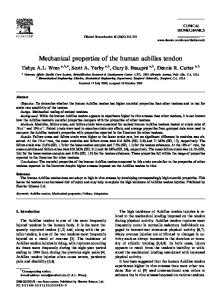
In both locomotor forms of movement, the body actions are cyclic, involving sequences in which the body is supported first by one leg and then the other. These sequences are defined by certain parameters. Typical parameters such as the stride and step are presented in Figure 8-25. A locomotor cycle or stride is defined by events in these sequences. A stride is defined as the interval from one event on one limb until the same event on the same limb in the following contact. Usually an event such as the first instant of foot contact defines the beginning of a stride. For example, a stride could be defined from heel contact of the right limb to subsequent heel contact on the right limb. The stride can be subdivided into steps. A step is a portion of the stride from an event occurring on one leg to the same event occurring on the opposite leg. For example, a step could be defined as foot contact on the right limb to foot contact on the left limb. Thus, two steps equal one stride, also called one gait cycle. Stride length and stride rate are among the most commonly studied linear kinematic parameters. The distance covered by one stride is the stride length, and the number of strides per minute is the stride rate. Running and walking velocity is the result of the relationship between stride rate and stride length. That is: Running speed � Stride length * Stride rate
Velocity can be increased by increasing stride length or stride rate or both. Examples of stride characteristics ranging from a slow walk up through a sprint are presented in Table 8-4, which clearly shows adjustments in stride rate and stride length that contribute to the increase in the velocity. The stride can be lengthened only so much; in fact, from walking speeds of 0.75 m/s on, pelvic rotation begins to contribute to the stride lengthening (31). Many studies (9,19,22,28) have shown that in running, both stride rate and stride length increase with increasing velocity, but the adjustment is not proportional at higher velocities. This is illustrated in Figure 8-26. For velocities up to 7 m/s, increases are linear, but at higher speeds, there is a smaller increment in stride length and a greater increment in stride rate. This indicates that when sprinting, runners increase their velocity by increasing their stride rate more than their stride length. A runner initially increases velocity by increasing stride length. However, there is a physical limit to how much an individual can increase stride length. To run faster, therefore, the runner must increase his or her stride rate. It has been shown that individuals chose a walking or running speed (preferred locomotor speed) and a preferred stride length at that preferred walking speed (18). Deviation from the preferred stride length at the preferred speed has serious consequences for the individual. Researchers have shown that increasing or decreasing stride length while keeping locomotor velocity constant
TA B L E 8 - 4 Stride Characteristic Comparison Between Walking
and Running Variable
Walking (17,25)
Running (22,25)
Sprint
Speed (m/s)
0.67�1.32
1.65�4.00
8.00�9.00
Stride length (m)
1.03�1.35
1.51�3.00
4.60�4.50
Cadence (steps/min)
79.00�118.00
132.00�200.00
Stride rate (Hz)
0.65�0.98
1.10�1.38
1.75�2.00
Cycle time (s)
1.55�1.02
0.91�0.73
0.57�0.50
Stance (% of gait cycle)
66.00�60.00
59.00�30.00
25.00�20.00
Swing (% of gait cycle)
34.00�40.00
41.00�70.00
75.00�80.00
Hamill_ch08_299-336.qxd
11/2/07
4:27 PM
Page 321
CHAPTER 8 Linear Kinematics
FIGURE 8-26 Changes in stride length and stride rate as a function of running velocity. (Adapted from Luhtanen, P., Komi, P. V. [1973]. Mechanical factors influencing running speed. In E. Asmussen, K. Jorgensen (Eds.). Biomechanics Vl-B. Baltimore: University Park Press.)
can increase the oxygen cost of locomotion (12,18). This is illustrated in Figure 8-27. Refer to the walking data in Appendix C. Calculate the step length, step frequency, stride length, stride frequency, and cadence (steps per minute). Calculate the walking velocity.
Each individual has a preferred speed at which he or she opts to start running instead of walking faster. This speed is usually somewhere around 2 m/s. The walking velocity at which individuals switch to a run is higher than the running velocity at which they shift back to a walk (20). Gait parameters are adjusted when physical or environmental conditions offer constraints to the gait cycle. For example, an individual with a limiting physical impairment
Oxygen consumption (1/min)
3.5
321
usually walks with a slower velocity and cadence by increasing the support phase of the cycle, decreasing the swing phase, and shortening the step length (25). Many individuals with cerebral palsy have significant gait restrictions evidenced by slow velocities, short strides, slow cadence, and more time spent in double support. Environmental factors also influence gait; for example, when the walking surface becomes slippery, most individuals reduce their step length. This minimizes the chance of falling by increasing the heel-strike angle with the ground and decreasing the potential for foot displacement on the slippery surface (3). The running and walking stride can be further subdivided into support (or stance) and nonsupport (or swing) phases. The support or stance phase occurs when the foot is in contact with the ground, that is, from the point of foot contact until the foot leaves the ground. The support phase is often subdivided further into heel strike followed by foot flat, midstance, heel rise, and toe-off. The nonsupport or swing phase occurs from the point that the foot leaves the ground until the same foot touches the ground again. The proportional time spent in the stance and swing phases varies considerably between walking and running. In walking, the percentage of the total stride time spent in support and swing is approximately 60% and 40%, respectively. These ratios change with increased speed in both running and walking (Table 8-4). The absolute time and the relative time (a percentage of the total stride time) spent in support decreases as running and walking speeds increase (1,2). Typical changes in relative time of the support phase in running range from 68% at a jogging pace to 54% at a moderate sprint to 47% at a full sprint. Time spent in the support and the swing phase is just one of the factors that distinguish walking from running. The other factor that determines if gait is a walk or a run is whether one foot is always on the ground or not. In walking, one foot is always on the ground, with a brief period when both feet are on the ground, creating a sequence of alternating single and double support (Fig. 8-28). In running, the person does not always have one foot on the ground; an airborne phase is followed by alternating single-support phases. Using MaxTRAQ, import the video file of the woman walking. What is the length of time spent in single support and double support during one stride? (Note: The time between frames is 0.0313 s).
3.0
2.5
VELOCITY CURVE
2.0
The linear kinematics of competitive running and walking has also been studied by biomechanists. In several cases, athletes were considered as a single point and no consideration was given to the movement of the arms and legs as individual units. Over the years, a number of researchers have tried to measure the velocity curve of a runner during a sprint race (14). A. V. Hill, who later won the Nobel
−20%
−10%
PFS
+10%
+20
Stride frequency FIGURE 8-27 Oxygen consumption as a function of stride frequency.
Hamill_ch08_299-336.qxd
322
11/2/07
4:27 PM
Page 322
SECTION III Mechanical Analysis of Human Motion
left initial contact
left toe-off
left toe-off
left swing phase
LEFT LEG
double support
RIGHT LEG
left stance phase
right single support
double support
left single support
double support
right swing phase
right stance phase
right toe-off
right initial contact
right initial contact
TIME
FIGURE 8-28 Support and double support during walking.
Prize in physiology, proposed a simple mathematical model to represent the velocity curve, and subsequent investigations have confirmed this model (Fig. 8-29). Most sprinters conform relatively closely to this model. At the start of the race, the runner’s velocity is zero. The velocity increases rapidly at first but then levels off to a constant value. This means that the runner accelerates rapidly at first, but the acceleration decreases toward the end of the run. The sprinter cannot increase velocity indefinitely throughout the race. In fact, the winner of a sprint race is usually the runner whose velocity decreases the least toward the end of the race. Figure 8-30 illustrates the displacement, velocity, and acceleration data for the women’s 100-m final in the 2000 Olympics. The graphs demonstrate similar characteristics for Marion Jones (Fig. 8-28A)
and Savatheda Fynes (Fig. 8-28B), even though they finished first and seventh, respectively. In a study of female sprinters (6), it was reported that the sprinters reached their maximum velocity between 23 and 37 m in a 100-m race. It was also reported that these sprinters lost an average of 7.3% from their maximum velocity in the final 10 m of the race. These two trends were also present in the 100-m women’s final shown in Figure 8-30. The fastest instantaneous velocity of a runner during a race has not yet been measured during competition. Average speed can be readily calculated, however. Marion Jones and Maurice Greene, in their gold medal performances at the 2000 Olympic Games, covered 100 m in 10.75 s and 9.87 s, respectively, for an average speed of 9.30 m/s and 10.13 m/s, or speeds equivalent to 20.8 mph and 22.7 mph, respectively. VARIATION OF VELOCITY DURING SPORTS
FIGURE 8-29 Hill’s proposed mathematical model of a sprint race velocity curve. (Adapted from Brancazio, P. J. [1984]. Sport Science. New York: Simon & Schuster.)
When average velocity was calculated over the race, note that this was not the velocity of the runner at every instant during the race. During a race, a runner contacts the ground numerous times, and it is important to note what occurs to the horizontal velocity during these ground contacts. The horizontal velocity of a runner during the support phase of the running stride from a study by Bates et al. (2) is presented in Figure 8-31A. An analysis of runners in this study indicated that the horizontal velocity decreased immediately at foot contact and continued to decrease during the first portion of the support period. As the runner’s limb extends in the latter portion of the support period, the
Hamill_ch08_299-336.qxd
11/2/07
4:27 PM
Page 323
CHAPTER 8 Linear Kinematics
(B) Savatheda Fynes
120
120
100
100
80
80
Distance (m)
Distance (m)
(A) Marion Jones
60 40
60 40 20
20 0
0 2
0
4
6
8
10
2
0
12
4
12
12
10
10 Velocity (m/sec)
Velocity (m/sec)
Time (sec)
8 6 4
6 Time (sec)
8
10
12
8
10
12
8
10
12
8 6 4 2
2
0
0 2
0
4
6
8
10
0
12
2
4
6 Time (sec)
Time (sec) 4.5 4 3.5 3 2.5 2 1.5 1 0.5 0 −0.5 −1
Acceleration (m/sec)
Acceleration (m/sec)
323
0
2
4
6
8
10
12
Time (sec)
4.5 4 3.5 3 2.5 2 1.5
1 0.5 0 −0.5 −1
0
2
4
6 Time (sec)
FIGURE 8-30 Distance (top), velocity (middle), and acceleration (bottom) curves for the 2000 Olympics women’s 100-m final performance of Marion Jones (A) and Savatheda Fynes (B). (Source of split times: http://sydney2000.nbcolympics.com/).
velocity increases. The corresponding acceleration–time graph of a runner during the support phase (Fig. 8-31B) shows distinct negative and positive accelerations. It can be seen that the runner instantaneously has zero acceleration during the support phase, representing the transition from negative acceleration to positive acceleration. This results from the runner’s slowing down during the first portion of support and speeding up in the latter portion. To maintain a constant average velocity, the runner must gain as much speed in the latter portion of the support phase as was lost in the first portion.
Linear Kinematics of the Golf Swing SWING CHARACTERISTICS
The purpose of the golf swing is to generate speed in the club head and to control the club head so that it is directed optimally for contact with the ball. Although many of the important biomechanical characteristics of the swing are angular, the linear kinematics of the club head ultimately determine the success of the golf swing.
Hamill_ch08_299-336.qxd
324
11/2/07
4:27 PM
Page 324
SECTION III Mechanical Analysis of Human Motion
800 m/s2 to prepare for contact. Contact is made with the ball at the original starting position (A), where the club head is still accelerating. Peak velocity is obtained shortly after impact. Club head velocities at impact in the range of 40 m/s are very possible; they can be much higher in some golfers. The time to complete the total swing may be in the range of 1000 ms, with the downswing phase accounting for 210 ms, or a little over 20% of the time. After impact is complete, the follow-through phase decelerates the club until the swing is terminated at C. VELOCITY AND ACCELERATION OF THE CLUB
Figure 8-33A illustrates the 3D velocity of the club (center of gravity) during the downswing phase (24). The motion of the club was recorded in three dimensions to determine linear kinematic characteristics toward the ball
Figure 8-32 shows the path of the club head in the swing. Starting at position A, the golfer brings the club back up behind and in front of the lead shoulder (B) to allow the club head to travel through a longer distance. The purpose of this backswing is to place the appropriate segments in an optimal position for force development and to establish the maximum range of motion for the subsequent downswing. In the downswing, the critical phase in the swing, the club head accelerates at rates greater than
A
Impact X
Velocity (m.s 1)
FIGURE 8-31 Changes in velocity (A) and acceleration (B) during the support phase of a running stride. (Adapted from Bates, B. T., et al. [1979]. Variations of velocity within the support phase of running. In J. Terauds and G. Dales (Eds.). Science in Athletics. Del Mar, CA: Academic.)
20 Z 0
200
100
Y
-20
Time (msec)
B
B C
Acceleration (m.s2)
Impact X
800
400
Y 0
100
200
Z
-400
Time (msec)
A FIGURE 8-32 The club head in a golf swing travels in a curved path through a considerable distance, allowing time to develop velocity in the club head.
FIGURE 8-33 Velocity–time (A) and acceleration–time (B) graphs of a driver segment center of gravity toward or away from the ball (X), vertically (Y), and in toward or away from the body (Z). (Adapted from Neal, R. J., Wilson, B. D. [1985]. 3D Kinematics and kinetics of the golf swing. International Journal of Sport Biomechanics, 1:221–232.)
Hamill_ch08_299-336.qxd
11/2/07
4:27 PM
Page 325
CHAPTER 8 Linear Kinematics
forward or backward (x), up or down (y), and away from or toward the golfer (z). In the initial portion of the downswing, with the club still up behind the head, the velocity in the x direction is backward, away from the ball, in the negative direction as the club is brought from the top of backswing around the body and toward the ball. In the last half of the downswing, the x velocity climbs sharply and becomes positive as the club is delivered toward the ball. The peak forward velocity is achieved after impact. The z or mediolateral velocity starts out negative, indicating that from the top of the backswing to approaching the halfway point in the downswing, the club is moving toward the golfer and then shifts positive as the club is swinging away from the golfer. This trend is opposite to that in the vertical direction, where the velocity in the y direction starts out with small movements upward and reverses to a downward movement as the club is brought down to the ball. The corresponding acceleration curves in Figure 8-33B identify critical phases in the swing at which maximal accelerations are obtained. Maximum acceleration in the direction of the ball (x) occurs 40 ms before impact, reaching a value of 870 m/s2 (24). Acceleration continues on through impact, even though it is small. There is also vertical acceleration, reaching maximum just before impact and still accelerating through the impact. These profiles or trends would look very much the same for all clubs, but there would be a reduction in the values such as club head velocity which decreases from the driver to the nine iron because of differences in club parameters.
Linear Kinematics of Wheelchair Propulsion CYCLE PARAMETERS
Many individuals with spinal cord injury or other serious musculoskeletal impairments use a wheelchair for locomotion. Propelling a manual wheelchair involves cyclic body actions, using sequences in which both hands are in contact with the rim or not. The typical wheelchair cycle includes a propulsive phase with the hand pushing on the hand rim of the wheelchair followed by a non-propulsive phase when the hand is brought back to the start of another propulsion phase. In the non-propulsive phase, three actions describe the phase, starting with disengagement
1
2 Sprinters
3
1
325
as the hand releases the hand rim at the end of propulsion followed by recovery as the hand is brought back up to the top of the hand rim to start the propulsion again and finally, contact when the hand touches the rim. The amount of time spent in contact and the range of displacement of the hand forward and backward varies with individual preferences and wheelchair configurations (e.g., seat position). Even in world-class athletes, the cycle patterns vary. Figure 8-34 shows displacement of the hand on the rim for different propulsive styles of six wheelchair athletes (16). The three sprinters typically used a backand-forth motion over the top of the hand rim, but the path of the disengagement from the rim varied as subjects’ hands moved through small or large loops when they moved the hand back to make contact with the rim for propulsion. In the three distance racers, the pattern of the hand motion was more circular but still varied quite significantly between individuals. PROPULSION STYLES
Two wheelchair propulsion styles have been identified (27). One is the pumping technique seen in the sprinters in Figure 8-35A, in which the hand moves back and forth horizontally with relatively large displacements away from the hand rim. The other popular technique is the circular technique (Fig. 8-35B), in which the hand moves in a circular path along the hand rim. The push phase in the circular pattern accounts for a larger percentage of the total propulsion cycle (43.0%) than the same phase in the pumping pattern (34.7%), suggesting that it may be more efficient. Vertical and horizontal displacements of the wrist, elbow, shoulder, and neck during wheelchair propulsion for a moderately active individual with T3–T4 paraplegia is presented in Figure 8-33A. In the propulsion cycle, the wrist travels forward and backward in a straight path, indicating a push pattern of propulsion. The neck moved forward and backward through a range of approximately 5.9 cm and at an average of about 1 cm for every 6.735 cm of wrist movement. Peak acceleration of the hand on the rim occurred close to the end of the push phase and is in the range of 32 m/s2. To increase the velocity of wheelchair propulsion, the cycle time is reduced by increasing the cycle frequency. This occurs as a result of shifting the start and end angles to the front of the hand rim without changing the angular
2 Distance racers
3
FIGURE 8-34 Hand displacement patterns for six Olympic wheelchair athletes illustrating differences in propulsion styles between sprinters (200 m) and distance racers (1500 m). (Adapted from Higgs, C. (1984). Propulsion of racing wheelchairs. In C. Scherrell (Ed.). Sport and Disabled Athletes. Champaign, IL: Human Kinetics, 165–172.)
Hamill_ch08_299-336.qxd
326
11/2/07
4:27 PM
Page 326
SECTION III Mechanical Analysis of Human Motion
FIGURE 8-35 Vertical and fore/aft displacements of the neck, shoulder, elbow, and wrist over multiple wheelchair propulsion cycles show differences between two subjects incorporating the pumping action style (A) and a circular action style (B) (Courtesy of Joe Bolewicz, RPT.)
components of the push angle (30). The pattern of action in the forearm changes from a push–pull pattern in the slower velocity to more of a push pattern with support from a continuous trunk flexion. Using MaxTRAQ, import the video file of the wheelchair athlete. Digitize the axle of the wheelchair in the frame at which the individual initiates the propulsion phase and then in the frame when the propulsion ends. Calculate the distance the wheelchair has traveled.
Projectile Motion Projectile motion refers to motion of bodies projected into the air. This type of motion implies that the projectile has no external forces acting on it except for gravity and air resistance. Projectile motion occurs in many activities, such as baseball, diving, figure skating, basketball, golf, and volleyball. The motion of a projectile is a special case of linear kinematics in which we know what changes in velocity and acceleration are going to occur after the object leaves the ground. For the following discussion, air resistance will be considered negligible because it is relatively small compared with gravity. Depending on the projectile, different kinematic questions may be asked. For example, in the long jump or the shot put, the horizontal displacement is critical. In the high jump and pole vaulting, however, vertical displacement must be maximized. In biomechanics, understanding the nature of projectile motion is critical.
GRAVITY
The force of gravity acting on a projectile results in constant vertical acceleration of the projectile. The acceleration due to gravity is approximately 9.81 m/s2 at sea level and results from the attraction of two masses, the earth and the object. Gravity uniformly accelerates a projectile toward the earth’s surface. However, not all objects that travel through the air are projectiles. Objects that are propelled, such as airplanes and objects that are aerodynamic such as a boomerang, are not generally classified as projectiles. TRAJECTORY OF A PROJECTILE
The flight path of a projectile is called its trajectory (Fig. 8-36A). The point in time at which an object becomes a projectile is referred to as the instant of release. Gravity continuously acts to change the vertical motion of the object after it has been released. The flight path followed by a projectile in the absence of air resistance is a parabola (Fig. 8-36A). A parabola is a curve that is symmetrical about an axis through its highest point. The highest point of a parabola is its apex. If gravity did not act on the projectile, it would continue to travel indefinitely with the same velocity as when it was released (Fig. 8-36B). In space, beyond the earth’s gravitational pull, a short firing burst of a vehicle’s rocket will result in a change in velocity. When the rocket ceases to fire, the velocity at that instant remains constant, resulting in zero acceleration. Because there is no gravity and no air resistance, the vehicle will continue on this path until the engine fires again.
Hamill_ch08_299-336.qxd
11/2/07
4:27 PM
Page 327
CHAPTER 8 Linear Kinematics
327
FIGURE 8-37 The factors influencing the trajectory of a projectile are projection velocity, projection angle, and projection height.
FIGURE 8-36 A. The parabolic trajectory of a projectile. B. Path a represents the trajectory of a projectile without the influence of gravity. Path b is a trajectory with gravity acting. Path b forms a parabola.
FACTORS INFLUENCING PROJECTILES
Three primary factors influence the trajectory of a projectile: the projection angle, projection velocity, and projection height (Fig. 8-37). Projection Angle The angle at which the object is released determines the shape of its trajectory. Projection angles generally vary from 0° (parallel to the ground) to 90° (perpendicular to the ground), although in some sporting activities, such as ski jumping, the projection angle is negative. If the projection angle is 0° (parallel to the horizontal), the trajectory is essentially the latter half of a parabola because it has zero vertical velocity and is immediately acted upon by gravity to pull it to the earth’s surface. On the other hand, if the projection angle is 90°, the object is projected straight up into the air with zero horizontal velocity. In this case, the parabola is so narrow as to form a straight line. If the projection angle is between 0° and 90°, the trajectory is parabolic. Figure 8-38 displays theoretical trajectories for an object projected at various angles with the same speed and height of projection.
The optimal angle of projection for a given activity is based on the purpose of the activity. Intuitively, it would appear that jumping over a relatively high object such as a high jump bar would require quite a steep projection angle. This has proved to be the case: High jumpers have a projection angle of 40° to 48° using the flop high jump technique (7). On the other hand, if one tried to jump for maximal horizontal distance such as in a long jump, the projection angle would be much smaller. This has also proved to be the case: Long jumpers have projection angles of 18° to 27° (12). Table 8-5 illustrates the projection
FIGURE 8-38 Theoretical trajectories of a projectile projected at different angles keeping velocity (15.2 m/s) and height (2.4 m) constant. (Adapted from Broer, M. R., Zernike, R. F. [1979]. Efficiency of Human Movement (4th Ed.). Philadelphia: WB Saunders.)
Hamill_ch08_299-336.qxd
328
11/2/07
4:27 PM
Page 328
SECTION III Mechanical Analysis of Human Motion
TA B L E 8 - 5 Projection Angles Used
in Selected Activities Activity
Angle (°)
Reference
Racing dive
5�22
14
Ski jumping
�4
19
Tennis serve
3�15
24
Discus
35�15
27
High jump (flop)
40�48
7
angles reported in the research literature for several activities. Positive angles of projection (i.e., angles greater than zero) indicate that the object is projected above the horizontal, and negative angles of projection refer to those less than zero or below the horizontal. For example, in a tennis serve, the serve is projected downward from the point of impact. Projection Velocity The velocity of the projectile at the instant of release determines the height and distance of the trajectory as long as all other factors are held constant. The resultant velocity of projection is usually calculated and given when discussing the factors that influence the flight of a projectile. The resultant velocity of projection is the vector sum of the horizontal and vertical velocities. It is necessary, however, to focus on the components of the velocity vector because they dictate the height of the trajectory and the distance the projectile will travel. Similar to other vectors, the velocity of projection has a vertical component (vy) and a horizontal component (vx). The magnitude of the vertical velocity is reduced by the effect of gravity (9.81 m/s for every second of upward flight). Gravity reduces the vertical velocity of the projectile until the velocity equals zero at the apex of the projectile’s trajectory. The vertical velocity component, therefore, determines the height of the apex of the trajectory. The vertical velocity also affects the time the projectile takes to reach that height and consequently the time to fall to earth. The horizontal component of the projection velocity is constant throughout the flight of the projectile. The range or the distance the projectile travels is determined by the product of the horizontal velocity and the flight time to the final position. The magnitude of the distance that the projectile travels is called the range of the projectile. For example, if a projectile is released at a horizontal velocity of 13.7 m/s, the projectile will have traveled 13.7 m in the first second, 27.4 m after 2 s, 40.1 m after 3 s, and so on. The angle of projection affects the relative magnitude of the horizontal and vertical velocity. If the angle of projection is 40° and the projection velocity is 13.7 m/s, the horizontal component of the projection velocity is the
product of the velocity and the cosine of the projection angle or 13.7 m/s and cosine 40° or 10.49 m/s. The vertical component is the product of the projection velocity and the sine of the projection angle (or 13.7 m/s) and sine 40° (or 8.81 m/s). To understand in general how the angle of projection affects the velocity components, consider that the cosine of 0° is 1 and decreases to zero as the angle increases. If the cosine of the angle is used to represent the horizontal velocity, the horizontal velocity decreases as the angle of projection increases from 0° to 90° (Fig. 8-39). Also, the sine of 0° is zero and increases to 1 as the angle increases. Consequently, if the sine of the angle is used to represent vertical velocity, the vertical velocity increases as the angle increases from 0° to 90° (Fig. 8-39). It can readily be seen that as the angle gets closer to 90°, the horizontal velocity becomes smaller and the vertical velocity becomes greater. As the angle gets closer to 0°, the horizontal velocity becomes greater and the vertical velocity gets smaller. At 45°, however, the sine and cosine of the angle are equal. For any given velocity, therefore, horizontal velocity equals vertical velocity. It would appear that 45° would be the optimum angle of projection because for any velocity, the horizontal and vertical velocities are equal. This is true under certain circumstances to be discussed in relation to projection height. Generally, if the maximum range of the projectile is critical, an angle to optimize the horizontal velocity, or an angle less than 45°, would be appropriate. Thus, in activities such as the long jump and shot putting, the optimal angle of projection is less than 45°. If the height of the projectile is important, an angle greater than 45° should be chosen. This is the case in activities such as high jumping. Projection Height The height of projection of a projectile is the difference in height between the vertical takeoff position and the vertical
FIGURE 8-39 Graph of sine and cosine values at angles from 0 to 90°. Sin 45° cosine 45°.
Hamill_ch08_299-336.qxd
11/2/07
4:27 PM
Page 329
CHAPTER 8 Linear Kinematics
landing position. Three situations greatly affect the shape of the trajectory. In each case, the trajectory is parabolic, but the shape of the parabola may not be completely symmetrical; that is, the first half of the parabola may not have the same shape as the second half. In the first case, the projectile is released and lands at the same height (Fig. 8-40A). The shape of the trajectory is symmetrical, so the time for the projectile to reach the apex from the point of release equals the time for the projectile to reach the ground from the apex. If a ball is kicked from the surface of a field and lands on the field’s surface, the relative projection height is zero, so the time up to the apex is equal to the time down from the apex. In the second situation, the projectile is released from a point higher than the surface on which it lands (Fig. 8-40B). The parabola is asymmetrical, with the initial portion to the apex less than the latter portion. In
329
this case, the time for the projectile to reach the apex is less than time to reach the ground from the apex. For example, if a shot putter releases the shot from 2.2 m above the ground and the shot lands on the ground, the height of projection is 2.2 m. In the third situation, the projectile is released from a point below the surface on which it lands (Fig. 8-40C). Again, the trajectory is asymmetrical, but now the initial portion to the apex of the trajectory is greater than the latter portion. Thus, the time for the projectile to reach the apex is greater than the time for the projectile to reach the ground from the apex. For example, if a ball is thrown from a height of 2.2 m and lands in a tree at a height of 4 m, the height of projection is 1.8 m. Generally, when the projection velocity and angle of projection are held constant, the higher the point of release, the longer the flight time. If the flight time is longer, the range is greater. Also, for maximum range, when the relative height of projection is zero, the optimum angle is 45°; when the projection height is above the landing height, the optimum angle is less than 45°; and when the projection height is below the landing height, the optimum angle is greater than 45°. The effect of landings that are lower than takeoffs is shown in Figure 8-38. OPTIMIZING PROJECTION CONDITIONS
FIGURE 8-40 Influence of projection height on the shape of the trajectory of a projectile.
To optimize the conditions for the release of a projectile, the purpose of the projectile must be considered. As discussed previously, the three primary factors that affect the flight of a projectile are interrelated and affect both the height of the trajectory and the distance traveled. Although it may seem intuitive that because the height of the apex and the length of the trajectory of the projectile are both affected by the projection velocity, increasing the projection velocity increases both of these parameters, this common perception is incorrect. The choice of an appropriate projection angle dictates whether the vertical or the horizontal velocity is increased with increasing projection velocity. In addition, the angle of projection can be affected by the height of projection. The relative importance of these factors is illustrated in the following example. If an athlete puts the shot with a velocity of 14 m/s at an angle of 40° from a height of 2.2 m, the distance of the throw is 22 m. If each factor is increased by a given percentage (10% in this case) as the other two factors are held constant, the relative importance of each factor may be calculated. Increasing the velocity to 15.4 m/s results in a throw of 26.2 m, increasing the angle to 44° results in a throw of 22 m, and increasing the height of projection to 2.4 m results in a throw of 22.2 m. It is readily evident that increasing the velocity of projection increases the range of the throw more substantially than increasing either the angle or the height of projection. The three factors are interrelated, however, and any change in one results in a change in the others.
Hamill_ch08_299-336.qxd
330
11/2/07
4:28 PM
Page 330
SECTION III Mechanical Analysis of Human Motion
Equations of Constant Acceleration When a projectile is traveling through the air, only gravity and air resistance act upon it. If air resistance is ignored, only gravity is considered to act on the projectile. The acceleration due to gravity is constant, so the projectile undergoes constant acceleration. Using the concepts from the previous section, equations of constant acceleration, or projectile motion, can be determined based on the definitions of velocity and acceleration. Three such expressions involve the interrelationships of the kinematic parameters time, position, velocity, and acceleration. These expressions are often referred to as the equations of constant acceleration. The first equation expresses final velocity as a function of the initial velocity, acceleration, and time. vf � vi � at where vf and vi refer to the final velocity and the initial velocity, a is the acceleration and t is time. In the second equation, position is expressed as a function of initial velocity, acceleration, and time. s = vit +
1 2 at 2
where vi is the initial velocity, t is time, and a is acceleration. The variable in this expression may refer to the horizontal or vertical case and is the change in position or the distance that the object travels from one position to another. This equation is derived by integrating the first equation. The last equation expresses final velocity as a function of initial velocity, acceleration, and position. vf 2 � vi 2 � 2as
where vf and vi refer to the final velocity and the initial velocity, a is acceleration, and s is the position. Each of the kinematic variables in this expression appeared in one or both of the previous equations. NUMERICAL EXAMPLE
The equations of constant acceleration use parameters that are basic to linear kinematics. The three equations of constant acceleration thus provide a useful method of analyzing projectile motion. If calculating the range of a projectile, for example, the following expression can be used: Range =
v2 * sin � * cos � + vx * 2(vy)2 + 2gh g
where v is velocity of projection, � is angle of projection, h is the height of release of the projection, and g is acceleration due to gravity. Suppose a shot putter releases the shot at an angle of 40° from a height of 2.2 m with a velocity of 13.3 m/s. Figure 8-41 illustrates what is known about the conditions of the projectile at the instant of projection and the shape of the trajectory based on our previous discussion. Using the previous equation, the range can be calculated as follows: 13.3 m/s2 * sin 40 * cos 40 � 10.19 m/s Range =
* 28.55 m/s2 + 2(9.81 m/s2)(2.2 m) 9.81 m/s2 176.89 * 0.6428 * 0.766 � 10.19
=
* 273.10 + 43.16 9.81
FIGURE 8-41 Conditions during the flight of the shot. Initial conditions are: v � 13.3 m/s, projection angle 40°, and projection height 2.2 m.
Hamill_ch08_299-336.qxd
11/2/07
4:28 PM
Page 331
CHAPTER 8 Linear Kinematics
87.09 + 10.19 * 10.78 9.81 87.09 + 109.84 = 9.81 � 20.07 m
a =
=
The same problem can be solved in seven steps using the equations of constant acceleration (see Appendix D).
Summary Biomechanics is a quantitative discipline. One type of quantitative analysis involves linear kinematics or the study of linear motion with respect to time. Linear kinematics involves the vector quantities, position, velocity, and acceleration and the scalar quantities displacement and speed. Displacement is defined as the change in position. Velocity is defined as the time rate of change of position and is calculated using the first central difference method as follows: si + 1 - si - 1 v = 2¢t Acceleration is defined as the time rate of change of velocity and is also calculated using the first central difference method as follows:
331
vi + 1 - vi - 1 2¢t
The process of calculating velocity from position and time or acceleration from velocity and time is called differentiation. Calculating the derivative via differentiation entails finding the slope of a line tangent to the parameter–time curve. The opposite process to differentiation is called integration. Velocity may be calculated as the integral of acceleration and position as the integral of velocity. Integration implies calculating the area under the parameter–time curve. The method of calculating the area under a parameter–time curve is called the Riemann sum. Projectile motion involves an object that undergoes constant acceleration because it is uniformly accelerated by gravity. The flight of a projectile, its height and distance, is affected by conditions at the point of release: the angle, velocity, and relative height of projection. Three equations govern constant acceleration. The first expresses final velocity, vf , as a function of initial velocity, vi; acceleration, a; and time, t. That is: vf � vi � at The second equation expresses position, s, as a function of initial velocity, vi; acceleration, a; and time, t. That is: s = vit +
1 2 at 2
Equation Review for Linear Kinematics Purpose
Given
Formula
Vector composition, magnitude
Horizontal and vertical components
r2 � x2 � y2
Vector composition, angle
Horizontal and vertical components
tan � � y/x
Vector resolution, vertical
Magnitude and direction of vector
y � r sin �
Vector resolution, horizontal
Magnitude and direction of vector
x � r cos �
Time between video frames
Camera frame, sampling rate
Time (s) � 1/frame rate
Calculate position
Starting position relative to origin, constant velocity (zero acceleration), time
s � si � vit
Calculate position
Starting position at origin, constant velocity (zero acceleration), time
s � vit
Calculate position
Initial velocity, time, constant acceleration
s � vit � 1/2at2
Calculate position
Initial velocity zero, time, constant acceleration
s � 1/2at2
Calculate average velocity
Displacement and time
v � x2 � x1/t2 � t1
Calculate average velocity
Initial and final velocity
v � vi � vf /2
Calculate final velocity
Initial velocity, constant acceleration, and time
vf � vi � at
Calculate final velocity
Starting velocity zero, constant acceleration, time
v � at
Calculate final velocity
Velocity at time � zero, constant acceleration, initial position relative to origin, final position
v � 冪vi2 � 2a(x � xi)
Calculate final velocity
Initial velocity zero, constant acceleration, initial and final position
vf2 � 2as v � 冪2a(x � xi)
Calculate acceleration
Final velocity and displacement
a � vf2/2d
Calculate average acceleration
Velocity and time
a � v2 � v1/t2 � t1
Calculate time
Displacement, constant acceleration
t � 冪2d/a
Calculate time in air for projectile beginning and landing at same height
Vertical velocity, constant acceleration
t � 2 vy /a
Calculate distance of projectile
Resultant velocity, initial angle of release, constant acceleration
s � r2 sin 2�/a
Hamill_ch08_299-336.qxd
332
11/2/07
4:28 PM
Page 332
SECTION III Mechanical Analysis of Human Motion
The third equation expresses final velocity, vf , as a function of initial velocity, vi; acceleration, a; and position, s. vf2
�
vi2
� 2as
These equations may be used to calculate the range of a projectile. However, a general equation for the range of a projectile is: Range =
v2 * sin � * cos � + vx * 2(vy)2 + 2gh g
20. ____ During running, stride length can affect metabolic cost. 21. ____ In a golf swing, the club head should be decelerating past contact with the ball. 22. ____ Maximum acceleration of the club head occurs at the moment of impact in a golf swing. 23. ____ Velocity of wheelchair propulsion is increased by increasing the length of the push on the wheel. 24. ____ Horizontal motion of a projectile is a special case of constant acceleration and determines the range of the projectile. 25. ____ Vertical velocity of a projectile is affected by gravity.
REVIEW QUESTIONS True or False 1. ____ Calculating the range of motion at the hip joint during stair ascent after visually observing the movement is a quantitative analysis. 2. ____ The motion of a parachutist in the air is an example of translational motion. 3. ____ The x- and y-axes in a two-dimensional rectangular reference system are always oriented vertically and horizontally, respectively. 4. ____ With a coordinate reference system originating at the hip joint, the axes of the coordinate system will always be horizontal and vertical. 5. ____ A 3D reference frame has three axes. 6. ____ Speed is a scalar quantity. 7. ____ Acceleration is defined as the time rate of change of position. 8. ____ Displacement is a scalar quantity. 9. ____ The slope of a line tangent to a curve indicates instantaneous velocity. 10. ____ Vectors can be added together graphically by placing the head of one vector at the tail of the other vector. 11. ____ The area under a displacement–time graph represents the average velocity. 12. ____ Positive acceleration relates to the direction of motion away from the origin. 13. ____ The point where the velocity is maximum in a velocity– time graph indicates the point where acceleration is maximum. 14. ____ Velocity is a measure of the area under the position– time curve. 15. ____ The steepness of the slope of a velocity–time curve is an indication of the magnitude of the acceleration. 16. ____ Stride length is always measured from the heel contact of one foot to the heel contact of the other foot. 17. ____ The support phase in walking accounts for the same percentage of the total cycle as in running. 18. ____ Walking speed is increased by first increasing stride length and then stride rate. 19. ____ Successful sprinters can usually increase their acceleration at the end of the race.
26. ____ Projectiles are never affected by air resistance.
Multiple Choice 1. Convert the rectangular coordinates of (122, 10) to polar coordinates. a. (11.49, 4.69) b. (122.4, 4.69) c. (122.4, 85.3) d. (11.49, 85.3) 2. Convert the polar coordinates of (135, 182) to rectangular coordinates. a. (�4.71, 134.9) b. (134.9, 4.71) c. (�134.9, 4.71) d. (4.71, 134.9) 3. Figure 8-11 depicts the path of a runner. If the runner starts and ends at the end of each block, and if each block is a square with lengths of 200 m, what is the magnitude of the resultant displacement of the runner? a. 1200 m b. 1150 m c. 894 m d. 900 m 4. A swimmer completes six laps in a 50-m swimming pool, finishing where he started. What were the linear distance and the linear displacement? a. Distance � 150 m; displacement � 150 m b. Distance � 300 m; displacement � 300 m c. Distance � 300 m; displacement � 0 d. None of the above 5. A basketball player shoots from beyond the 3-point arc. The ball leaves the hand with an initial velocity of 8 m/s angled 52° from the horizontal. What are the horizontal and vertical velocity of the basketball? a. vx � 6.3 m/s vy � 4.9 m/s b. vx � 4.9 m/s vy � 6.3 m/s c. vx � 6.0 m/s vy � 5.0 m/s d. vx � 5.0 m/s vy � 6.0 m/s 6. At takeoff, the horizontal and vertical velocities of a long jumper are 7.6 m/s and 3 m/s, respectively. What are the resultant velocity and angle of takeoff? a. v � 8.17 m/s � � 11.9° b. v � 7.2 m/s � � 11.9° c. v � 7.2 m/s � � 21.5° d. v � 8.17 m/s � � 21.5°
Hamill_ch08_299-336.qxd
11/2/07
4:28 PM
Page 333
CHAPTER 8 Linear Kinematics
7. Given a right triangle with hypotenuse � 12.5 cm, side Y � 7.2 cm, find the length of side X and the size of the other two angles. a. Side X � 14.42 cm �1 � 31.7° �2 � 53.2° b. Side X � 10.2 cm �1 � 35.2° �2 � 54.8° c. Side X � 12.5 cm �1 � 54.8° �2 � 35.2° d. Side X � 14.42 cm �1 � 53.2° �2 � 31.7° 8. Suppose an individual moves from point s1 (6, 9) to point s2 (11, 10) to point s3 (5, 6). What are the horizontal, vertical, and resultant displacements? a. -Horizontal � 11 units; vertical � 5 units; resultant � 12.1 units b. -Horizontal � 1 unit; vertical � 3 units; resultant � 3.16 units c. -Horizontal � ~1 unit; vertical � ~3 units; resultant � 3.16 units d. -Horizontal � ~11 units; vertical � ~5 units; resultant � 12.1 units 9. Combine the following two vectors to find the resultant vector. Vector A � 7.4 units at 30° and vector B � 11.1 units at 120°. a. Resultant � 13.34 units; � � 86.3° b. Resultant � 18.49 units; � � 60.0° c. Resultant � 17.89 units; � � 48.1° d. Resultant � 17.89 units; � � 41.9° 10. An individual drives 50 km in 72 minutes. What was the average speed in meters per second? a. 1.157 b. 11.57 c. 69.44 d. 694.44 11. A train accelerates from rest at a constant rate of 10 m/s2. How fast is it going after 5 s? a. 500 m/s b. 50 m/s c. 5 m/s d. 55 m/s 12. The initial velocity of a projectile is 45 m/s at 72°. How high above the ground and how far horizontally is the object when it is 4.7 s into the flight? a. Vertical � 92.78 m; horizontal � 65.38 m b. Vertical � 87.54 m; horizontal � 62.34 m c. Vertical � 94.56 m; horizontal � 70.11 m d. Vertical � 91.56 m; horizontal � 64.87 m 13. A triple jumper needs a velocity of 9 m/s to make a good jump. If he is accelerating at 1.7 m/s2, how much time does he need to reach the velocity? a. 4.79 s b. 5.33 s c. 5.18 s d. 5.29 s 14. A vaulter is trying to reach a velocity of 8 m/s at the end of a 15-m runway. How quickly must she accelerate? a. 2.13 m/s2 b. 1.82 m/s2 c. 1.90 m/s2 d. 2.09 m/s2 15. A sprinter starts from rest and reaches a maximum velocity of 7.4 m/s in 2.5 s. What was the average acceleration from rest to maximum velocity?
a. b. c. d.
3.01 2.94 2.87 2.96
333
m/s2 m/s2 m/s2 m/s2
16. A high jumper takes off with a vertical velocity of 4.2 m/s. How long does it take the jumper to reach the peak height of the jump? a. 0.86 s b. 0.79 s c. 0.43 s d. 0.37 s 17. Golf ball A is driven straight out from a tee box that is 2 m above the fairway. At the instant the club contacts the ball, another golfer drops ball B from a height of 2 m. Which ball will contact the ground first? a. Ball A b. Ball B c. Both balls will contact at the same time Questions 18 to 24: A baseball is thrown with a velocity of 31 m/s at an angle of 40° from a height of 1.8 m. 18. Calculate the vertical and horizontal velocity components. a. vx � 18.65 m/s vy � 12.58 m/s b. vx � 12.58 m/s vy � 18.65 m/s c. vx � 19.93 m/s vy � 23.75 m/s d. vx � 23.75 m/s vy � 19.93 m/s 19. Calculate the time to peak trajectory. a. 2.03 s b. 2.42 s c. 2.32 s d. 1.90 s 20. Calculate the height of the trajectory from the point of release. a. 17.73 m b. 28.73 m c. 22.01 m d. 20.21 m 21. Calculate the total height of the parabola. a. 22.01 m b. 30.52 m c. 19.43 m d. 24.25 m 22. Calculate the time from the apex to the ground. a. 1.99 s b. 2.49 s c. 2.12 s d. 2.22 s 23. Calculate the total flight time. a. 3.89 s b. 4.91 s c. 4.15 s d. 4.54 s 24. Calculate the range of the throw. a. 98.53 m b. 48.94 m c. 63.33 m d. 115.8 m 25. A baseball leaving the bat at 46° at a height of 1.2 m from the ground clears a 3-m high wall 125 meters from home
Hamill_ch08_299-336.qxd
334
11/2/07
4:28 PM
Page 334
SECTION III Mechanical Analysis of Human Motion
plate. What is the initial velocity of the ball (ignoring air resistance)? a. 37.3 m/s b. 34.9 m/s c. 35.02 m/s d. 36.9 m/s
REFERENCES 1. Bates, B. T., Haven, B. H. (1974). Effects of fatigue on the mechanical characteristics of highly skilled female runners. In R. C. Nelson, C. A. Morehouse (Eds.). Biomechanics IV. Baltimore: University Park Press, 119–125. 2. Bates, B. T., et al. (1979). Variations of velocity within the support phase of running. In J. Terauds and G. Dales (Eds.). Science in Athletics. Del Mar, CA: Academic, 51–59. 3. Brady, R. A., et al. (2000). Foot displacement but not velocity predicts the outcome of a slip induced in young subjects while walking. Journal of Biomechanics, 33:803–808. 4. Brancazio, P. J. (1984). Sport Science. New York: Simon & Schuster. 5. Broer, M. R., Zernike, R. F. Efficiency of Human Movement (4th ed.). Philadelphia: Saunders College, 1979. 6. Chow, J. W. (1987). Maximum speed of female high school runners. International Journal of Sports Biomechanics, 3:110–127. 7. Dapena, J. (1980). Mechanics of translation in the Fosbury flop. Medicine and Science in Sports and Exercise, 12:37–44. 8. Dapena, J., Chung, C. S. (1988). Vertical and radial motions of the body during the take-off phase of high jumping. Medicine and Science in Sports and Exercise, 20:290–302. 9. Elliott, B. C., Blanksby, B. A. (1979). A biomechanical analysis of the male jogging action. Journal of Human Movement Studies, 5:42–51. 10. Elliott, B., et al. (1986). A three-dimensional cinematographic analysis of the fastball and curveball pitches in baseball. International Journal of Sport Biomechanics, 2:20–28. 11. Fukashiro, S., Komi, P. V. (1987). Joint moment and mechanical power flow of the lower limb during vertical jump. International Journal of Sports Medicine, 8:15–21. 12. Hamill, J., et al. (1995). Shock attenuation and stride frequency during running. Human Movement Science 14:45–60. 13. Hay, J. G. (1986). The biomechanics of the long jump. Exercise and Sport Science Review, 401–446. 14. Henry, F. M., Trafton, I. (1951). The velocity curve of sprint running. Research Quarterly, 23:409–422.
15. Heusner, W. W. (1959). Theoretical specifications for the racing dive: Optimum angle for take-off. Research Quarterly, 30:25–37. 16. Higgs, C. (1984). Propulsion of racing wheelchairs. In C. Sherrel (Ed.). Sport and Disabled Athletes. Champaign, IL: Human Kinetics, 165–172. 17. Holden, J. P., et al. (1997). Changes in knee joint function over a wide range of walking speeds. Clinical Biomechanics, 12:375–382. 18. Holt, K. G., et al. (1991). Predicting the minimal energy cost of human walking. Medicine and Science in Sports and Exercise 23(4):491–498. 19. Hoshikawa, T., et al. (1973). Analysis of running patterns in relation to speed. In Medicine and Sport Vol. 8: Biomechanics III. Basel: Karger, 342–348. 20. Hreljac, A. (1993). Preferred and energetically optimal gait transition speeds in human locomotion. Medicine and Science in Sports and Exercise, 25:1158–1162. 21. Komi, P. V., et al. (1974). Biomechanics of ski-jumping. Jyvaskyla, Finland: University of Jyvaskyla, 25–29. 22. Luhtanen, P., Komi, P. V. (1973). Mechanical factors influencing running speed. In E. Asmussen, K. Jorgensen (Eds.). Biomechanics Vl-B. Baltimore: University Park Press, 23–29. 23. Mason, B. R., et al. (1996). Biomechanical golf swing analysis. In R. Bauer (ed.). XIII International Symposium for Biomechanics in Sport: Proceedings. Thunder Bay, Ontario: International Society for Biomechanics in Sport, 67–70. 24. Neal, R. J., Wilson, B. D. (1985). 3D Kinematics and kinetics of the golf swing. International Journal of Sport Biomechanics, 1:221–232. 25. Ounpuu, S. (1994). The biomechanics of walking and running. Clinics in Sports Medicine, 13:843–863. 26. Owens, M. S., Lee, H. Y. (1969). A determination of velocities and angles of projection for the tennis serve. Research Quarterly, 40:750–754. 27. Sanderson, D. J., Sommer, H. J. (1985). Kinematic features of wheelchair propulsion. Journal of Biomechanics, 18:423–429. 28. Sinning, W. E., Forsyth, H. L.(1970). Lower limb actions while running at different velocities. Medicine and Science in Sports, 2:28–34. 29. Terauds, J. (1975). Some release characteristics of international discus throwing. Track and Field Review, 75:54–57. 30. Vanlandewijck, Y. C., et al. (1994). Wheelchair propulsion efficiency: Movement pattern adaptations to speed changes. Medicine and Science in Sports and Exercise, 26:1373–1381. 31. Wagenaar, R. C., Emmerik, R. E. A. (2000). Resonant frequencies of arms and legs identify different walking patterns. Journal of Biomechanics, 33:853–861.
Hamill_ch08_299-336.qxd
11/2/07
4:28 PM
Page 335
CHAPTER 8 Linear Kinematics
335
G L O S S A RY Abscissa: The vertical axis of a coordinate system. Apex: The highest point of a parabola and the highest point a projectile reaches in its trajectory. Calculus: A method of calculating the derivative or integral of a function. Cartesian Coordinate System: An x, y, z reference system with either two or three axes in which a point may be located as a distance from each of the axes. Cosine of an Angle: In a right triangle, the ratio of the side adjacent to the angle and the hypotenuse. Curvilinear Motion: Linear motion along a curved path. Derivative: The result of differentiation—the slope of a line– either a secant or a tangent, on a parameter–time curve. Differentiation: The mathematical process of calculating a derivative. Digitization: The process of applying x, y coordinates to points on a video frame. Dimension: A term denoting the nature of a measurable quantity. First Central Difference Method: A method of calculating the average slope over two time intervals, as in generating velocity from position–time data or acceleration from velocity–time data. Instantaneous Linear Acceleration: The slope of a line tangent to a velocity–time curve. Instantaneous Linear Velocity: The slope of a line tangent to a position–time curve. Integral: The result of the process of integration; the area under a parameter–time curve. Integration: The mathematical process of calculating an integral. Kinematics: The area of study that examines the spatial and temporal components of motion. Limit: The derivative of a function when the change in time approaches zero. Linear Acceleration: The time rate of change of linear velocity. Linear Distance: The length of an actual path. Linear Displacement: A vector representing the straightline distance and direction from one position to another. Linear Motion: See Translation. Linear Kinematics: The description of linear motion involving position, velocity, and acceleration. Linear Velocity: The time rate of change of linear position. Midstance: The point during locomotor support when the center of mass is directly over the foot. Motion: The progressive change in position of an object. Ordinate: The horizontal axis of a coordinate system. Projectile: An object that has been projected into the air. Projectile Motion: The motion of a projectile. Projection Angle: The angle at which a projectile is released.
Projection Height: The difference between the heights at which a projectile is released and at which it lands. Projection Velocity: The velocity at which a projectile is released. Pythagorean Theorem: A mathematical description of the relationship among the sides of a right triangle. That is, a2 � b2 � c2, where a is the hypotenuse and b and c are the other sides of the triangle. Qualitative Analysis: A nonnumeric description or evaluation of movement that is based on direct observation. Quantitative Analysis: A numeric description or evaluation of movement based on data collected during execution of the movement. Range: The distance a projectile travels. Resultant: The sum of two vectors. Riemann Sum: A mathematical process by which the area under a parameter–time curve can be calculated, given that the time interval, dt, is small. Rise: The change in a parameter between two successive time intervals. Run: The change in time between two successive locations of parameter. Scalar: A quantity that is defined by its magnitude alone. Secant: A line that intersects a curve at two places. Sine of an Angle: In a right triangle, the ratio of the side opposite the angle and the hypotenuse. Slope: The ratio of the rise to the run. Speed: The magnitude of the velocity vector. Stance: See Support. Step: A portion of a stride from an event occurring on one leg to the same event on the opposite leg. Stride: A gait cycle lasting from an event by one limb to the next occurrence of that event by the same limb, as from heel strike to heel strike on the right foot. Stride Length: The distance traveled during one stride. Stride Rate: The number of strides per minute. Support: The phase of the gait cycle when the foot is in contact with the ground. Swing: See Nonsupport. Tangent: A line that touches a curve at only one place. Trajectory: The flight path of a projectile. Translation: Motion in a straight or curved path where different regions of the object move the same distance in the same time interval. Nonsupport: A phase of the gait cycle in which the leg is not supported on the ground. Vector: A quantity that is defined by both its magnitude and its direction. Parabola: A curve that describes the trajectory of a projectile.
Hamill_ch08_299-336.qxd
11/2/07
4:28 PM
Page 336