Land Evaluation for Agricultural Production in the Tropics
A Two-Level Crop Growth Model for Annual Crops A. Verdoodt & E. Van Ranst
Ghent University Laboratory of Soil Science
In order to cope with the increasing population pressure, farmers of many tropical developing countries face a dilemma: How to achieve a maximum crop yield with a minimum of critical natural resources such as land, water and nutrients. Building upon fundamental knowledge about the plant physiology and the behaviour of water in the plant-atmosphere-soil continuum, the authors developed a two-level crop growth model, describing the daily biomass production of annual crops under optimal and rainfed environmental conditions. The model incorporates several procedures estimating the rooting depth and leaf area index, describing the daily soil moisture within a multi-layered water balance and finally simulating the impact of water or oxygen shortage on crop development and yield. Sensitivity analysis and model validation were performed using the extended natural resources database of Rwanda.
Title of related interest:
Land Evaluation for Agricultural Production in the Tropics. A Large-Scale Land Suitability Classification for Rwanda. A. Verdoodt and E. Van Ranst Laboratory of Soil Science, Ghent University, Gent ISBN 90-76769-89-3
Land Evaluation for Agricultural Production in the Tropics
A Two-Level Crop Growth Model for Annual Crops
A. Verdoodt & E. Van Ranst
Ghent University Laboratory of Soil Science
Published by the Laboratory of Soil Science, Ghent University Krijgslaan 281 S8, B-9000 Gent, Belgium
Printed in Belgium
© Laboratory of Soil Science, Ghent University 2003
Cover photographer: Romain Baertsoen in: Omer Marchal (1987). Au Rwanda - La Vie Quotidienne au Pays du Nil Rouge. Didier Hatier, Brussels
ISBN 90-76769-88-5 No part of this publication may be reproduced in any form or by any means, electronically, mechanically, by photocopying, recording or otherwise, without the prior permission of the copyright owners.
Contents
CONTENTS
CHAPTER 1. INTRODUCTION 1.1.
Focus on crop growth modelling................................................................................... 1
1.2.
Focus on Rwanda ........................................................................................................... 2
1.3.
Outline............................................................................................................................. 3
CHAPTER 2. FROM CROP GROWTH MODELS TO YIELD GAP ANALYSIS 2.1.
Crop growth simulation models.................................................................................... 5
2.2.
Land evaluation.............................................................................................................. 6
2.3.
Sustainable land management ...................................................................................... 7
2.4.
Land quality and land quality indicators..................................................................... 8
2.4.1.
Nutrient balance ............................................................................................................... 9
2.4.2.
Yield gap .......................................................................................................................... 9
2.4.3.
Agricultural land use intensity and land use diversity ..................................................... 9
2.4.4.
Land cover...................................................................................................................... 10
2.5.
Yield gap analysis......................................................................................................... 11
2.5.1.
Potential production situation ........................................................................................ 12
2.5.2.
Water-limited production situation ................................................................................ 12
2.5.3.
Nutrient-limited production situation............................................................................. 12
2.5.4.
Actual yield .................................................................................................................... 12
i
Contents
CHAPTER 3. RADIATION-THERMAL PRODUCTION POTENTIAL 3.1.
Introduction .................................................................................................................. 15
3.2.
Photosynthesis .............................................................................................................. 17
3.2.1.
Photosynthesis light response of individual leaves ........................................................ 18
3.2.2.
Distribution of light through the canopy ........................................................................ 20
3.2.3.
Gross assimilation .......................................................................................................... 23
3.2.4.
Calculation of astronomical parameters......................................................................... 28
3.2.5.
Gross photosynthetic rate of a fully developed canopy ................................................. 30
3.2.6.
Gross photosynthetic rate of a non-closed crop surface................................................. 35
3.2.7.
Actual gross canopy assimilation rate............................................................................ 36
3.3.
Respiration.................................................................................................................... 38
3.3.1.
Maintenance respiration ................................................................................................. 38
3.3.2.
Growth respiration ......................................................................................................... 40
3.3.3.
Net assimilation.............................................................................................................. 40
3.4.
Yield efficiency ............................................................................................................. 42
3.5.
Crop development ........................................................................................................ 43
3.5.1.
Phenological stages ........................................................................................................ 43
3.5.2.
Partitioning of assimilates and leaf growth .................................................................... 45
3.5.3.
Initialisation ................................................................................................................... 49
3.6.
Sensitivity analysis ....................................................................................................... 50
3.6.1.
Objectives....................................................................................................................... 50
3.6.2.
Input data........................................................................................................................ 50
3.6.3.
Estimation of solar radiation .......................................................................................... 52
3.6.4.
Estimation of gross photosynthetic rate of a fully developed canopy............................ 53
3.6.5.
Estimation of actual gross canopy photosynthetic rate .................................................. 57
ii
Contents
3.6.6.
Estimation of maintenance respiration rate .................................................................... 60
3.6.7.
Estimation of net assimilation rate, growth respiration rate and growth rate................. 61
3.6.8.
Yield estimation for 5 crops, sown in different cropping seasons and in different altitudinal regions........................................................................................................... 63
3.7.
Discussion...................................................................................................................... 72
3.7.1.
Assumptions and limitations .......................................................................................... 72
3.7.2.
Yield prediction.............................................................................................................. 74
3.7.3.
Conclusion ..................................................................................................................... 75
CHAPTER 4. WATER-LIMITED PRODUCTION POTENTIAL 4.1.
Introduction .................................................................................................................. 77
4.2.
Soil-plant atmosphere continuum............................................................................... 80
4.2.1.
Electrical analog............................................................................................................. 80
4.2.2.
Water balance................................................................................................................. 81
4.3.
Components of the water balance............................................................................... 86
4.3.1.
Soil compartments.......................................................................................................... 86
4.3.2.
Processes ........................................................................................................................ 87
4.4.
Evapotranspiration ...................................................................................................... 90
4.4.1.
Selection of the calculation procedure ........................................................................... 90
4.4.2.
Reference evapotranspiration......................................................................................... 90
4.4.3.
Maximum transpiration.................................................................................................. 97
4.4.4.
Maximum evaporation ................................................................................................... 99
4.4.5.
Maximum evapotranspiration ...................................................................................... 101
4.4.6.
Rooting depth ............................................................................................................... 101
4.4.7.
Actual transpiration...................................................................................................... 106
iii
Contents
4.4.8.
Actual evaporation ....................................................................................................... 112
4.5.
Percolation .................................................................................................................. 114
4.5.1.
Preliminary percolation ................................................................................................ 114
4.5.2.
Maximum percolation .................................................................................................. 114
4.5.3.
Actual percolation ........................................................................................................ 115
4.6.
Infiltration, surface storage, run-off......................................................................... 116
4.6.1.
Infiltration .................................................................................................................... 116
4.6.2.
Surface storage ............................................................................................................. 117
4.6.3.
Run-off ......................................................................................................................... 119
4.7.
Capillary rise .............................................................................................................. 120
4.7.1.
Groundwater level........................................................................................................ 120
4.7.2.
Capillary rise above the groundwater table.................................................................. 120
4.7.3.
Modelling groundwater influence ................................................................................ 122
4.8.
Crop growth in water stress conditions.................................................................... 125
4.8.1.
Relationship between water uptake and crop production............................................. 125
4.8.2.
Actual gross biomass photosynthesis rate.................................................................... 125
4.8.3.
Development of crop components................................................................................ 127
4.8.4.
Length of crop cycle..................................................................................................... 129
4.9.
Initialisation ................................................................................................................ 130
4.10.
Sensitivity analysis ..................................................................................................... 131
4.10.1. Objectives..................................................................................................................... 131 4.10.2. Input data..................................................................................................................... 131 4.10.3. Sowing versus emergence ............................................................................................ 138
iv
Contents
4.10.4. Climate ......................................................................................................................... 138 4.10.5. Landscape..................................................................................................................... 146 4.10.6. Soil ............................................................................................................................... 152 4.10.7. Management................................................................................................................. 162 4.10.8. Crop.............................................................................................................................. 167 4.10.9. DAMUWAB versus DESIWAB.................................................................................. 177 4.11.
Discussion.................................................................................................................... 188
4.11.1. DAMUWAB features................................................................................................... 188 4.11.2. DAMUWAB performance ........................................................................................... 190 4.11.3. Conclusions .................................................................................................................. 191 CHAPTER 5. CONCLUSIONS 5.1.
Performance of the elaborated crop growth model ................................................ 193
5.2.
Agricultural potential of the arable land in Rwanda.............................................. 195
REFERENCES........................................................................................................................ 197
ANNEX I. RPP – INPUT DATA AND EXAMPLE I.1.
Input data.................................................................................................................... 205
I.2.
Calculation of the leaf area index ............................................................................. 206
I.3.
Calculation of the photosynthetic active radiation.................................................. 207
I.4.
Gross assimilation ...................................................................................................... 210
I.5.
Maintenance respiration............................................................................................ 216
I.6.
Growth and dry matter accumulation ..................................................................... 217
v
Contents
I.7.
Harvest index and yield of economically useful crop organs ................................. 218
ANNEX II. WPP – INPUT DATA AND EXAMPLE II.1.
Soil profiles ................................................................................................................. 219
II.2.
Climatic records ......................................................................................................... 225
II.3.
DAMUWAB: an example .......................................................................................... 233
II.3.1. Input data ........................................................................................................................ 233 II.3.2. Water balance from August to October .......................................................................... 234 II.3.3. Water balance during the crop cycle .............................................................................. 241 II.3.4. Dry beans yield during season A of the agricultural year 1987...................................... 254
vi
Chapter 1
Introduction
CHAPTER 1. INTRODUCTION
1.1.
Focus on crop growth modelling
International agricultural research is focussed on the elaboration of multidisciplinary models and technologies, guiding the way to rational and sustainable land use, in order to cope with the rapid population growth and declining agricultural productivity, affecting the livelihoods and very survival of millions of rural households throughout the developing world. Whereas the necessary input data for the agricultural research mainly become available through the realisation and updating of digital natural resources databases, the methods for investigation of the agricultural potential of land are found in the research topics on land evaluation and crop growth modelling. The multiple-step crop growth model described by Tang et al. (1992) allows the estimation of crop yields and identification of the relative importance of different production factors, taking into account climate, soil, landform, and also the impact of socio-economic settings and preferences. It has been applied successfully for the assessment of the agricultural production potential in many tropical countries. Nevertheless, application of this model in the semi-arid region of the Eastern Cape, South Africa, highlighted some serious limitations with respect to the simulation of the soil water balance during periods of erratic rainfall (Verdoodt, 1999). When assessing of the potential food self-sufficiency in Rwanda, Central Africa (Goethals, 2002; Vekeman, 2002), other serious limitations of the model were highlighted. The applied water balance was only valid for freely drained soils, leading to a serious underestimation of the water availability of the valley soils during the dry season, while waterlogging may occur during periods of high rainfall.
1
Chapter 1
1.2.
Focus on Rwanda
Knowledge of the soils, their properties and their spatial distribution, is indispensable for the agricultural development of Rwanda as it opens opportunities for a more rational management of the land resources. During the soil survey project entitled “Carte Pédologique du Rwanda”, started in 1981 and realised through a cooperation between the Rwandan Ministry of Agriculture, Livestock and Forestry and the Belgian government, much of this essential soil information at scale 1:50,000 has been gathered, analysed and stored in a large digital database. In addition, this database is being extended with information on the hydrology, topography and climate. The resulting natural resources database has become the key instrument for the description of the physical environment that farmers face in the different agricultural regions of the country and for the evaluation of the agricultural potentialities (Van Ranst et al., 2001). Whereas qualitative land evaluation methods are useful tools in the research for regionalisation and diversification of the agriculture, they are incapable of simulating the impact of the smallscale temporal and spatial changes in climate, topography and soil within mountainous Rwanda. An integration of quantitative land evaluation methodologies with more detailed crop simulation models was required. The erratic rainfall and high variability in soil properties that occurred within most soil units, further stressed the importance of designing a fine–tuned crop growth model.
2
Introduction
1.3.
Outline
In view of looking for solutions to the methodological shortcomings of existing land evaluation tools and to the current problems in the Rwandan agriculture, this book describes the elaboration of a two-level crop growth model. The new model was elaborated describing crop growth at a daily temporal scale and making use of a soil profile database containing standard analytical data. At this level of detail, land is characterised by daily climatic conditions, slope gradient, properties of the soil series and management practices of the farmers selecting a specific crop and sowing date. Actually, the model consists of two hierarchical production situations: the radiation-thermal production potential and the water-limited production potential. The sensitivity analysis and validation have been performed using the extended digital natural resources database of Rwanda. Chapter 2 offers the reader some background information on the status of land evaluation tools and crop growth models in the current research activities focussed by the scientific community. Chapter 3 and 4 describe the two production situations of the crop growth model. The first chapter deals with the radiation-thermal production potential, the latter describes the waterlimited production potential. Both include the elaboration of the modelling procedures, with references to other existing models and an in-depth sensitivity analysis. They conclude with a comparison of the simulated production potentials with reported yields and an evaluation of the model performance. A summary of the general results and final remarks has been given in chapter 5.
3
Chapter 2
From Crop Growth Models to Yield Gap Analysis
CHAPTER 2. FROM CROP GROWTH MODELS TO YIELD GAP ANALYSIS
Why is so much water lost by transpiration to grow a crop? Because the molecular skeletons of virtually all organic matter in plants consist of carbon atoms that must come from the atmosphere. They enter the plant as CO2 through stomatal pores, mostly on leaf surfaces, and water exits by diffusion through the same pores as long as they are open. You could say that the plant faces a dilemma: how to get as much as CO2 as possible from an atmosphere in which it is extremely dilute and at the same time retain as much water as possible. The agriculturalist faces a similar challenge: how to achieve a maximum crop yield with a minimum of irrigation or rainfall, a critical natural resource (Sinclair et al., 1984). Moreover, agricultural land-use decisions present several challenges and decision makers must often consider multiple and frequently conflicting agronomic, economic, social, and environmental goals.
2.1.
Crop growth simulation models
By the end of the 1960s, computers had evolved sufficiently to allow and even stimulate the first attempts to synthesize the detailed knowledge on plant physiological processes, in order to explain the functioning of crops as a whole. Insights into various processes were expressed using mathematical equations and integrated in so-called simulation models. These first models were meant to increase the understanding of crop behaviour by explaining crop growth and development in terms of the underlying physiological mechanisms. Over the years, new insights and different research questions motivated the further development of crop growth simulation models. In addition to their explanatory function, the applicability of well-tested models for extrapolation and prediction was quickly recognized. More applicationoriented models were developed driven by a demand for tactical and strategic decision support, yield forecasting, and explorative scenario studies (Bouman et al., 1996).
5
Chapter 2
2.2.
Land evaluation
In 1976, the Food and Agriculture Organization (FAO) published ‘A framework for land evaluation’ that provides principles for the qualitative evaluation of the suitability of land for alternative uses based on biophysical, economic and social criteria (Hansen et al., 1998). The term land is a central element in the definition of land evaluation and sustainable land management. Land is an area of the earth’s surface, including all elements of the physical and biological environment that influence land use. Land refers not only to soil, but also to landforms, climate, hydrology, vegetation and fauna, together with land improvements, such as terraces and drainage works (Sombroek, 1995). The term land evaluation has been used to describe many concepts and analytical procedures. Most frequently its main objective is to appraise the potential of land for alternative kinds of land use by a systematic comparison of the requirements of this land use with the resources offered by the land (Dent and Young, 1981). More specifically, land evaluation was intended to optimise particularly the productive function of the land and to obtain other important land information at the same time (Hurni, 2000). And thus, quantitative land evaluation methods were developed, using more detailed technical procedures such as computer models simulating crop growth, soil water flow and nutrient uptake (Van Lanen et al., 1992).
6
From Crop Growth Models to Yield Gap Analysis
2.3.
Sustainable land management
The term sustainable land management (SLM) emerged later as a follow up to the global discussion on sustainable development initiated by the Brundtland Commission. Sustainable development was defined as “development that meets the needs of the present without compromising the ability of future generations to meet their own needs” (WCED, 1987; Smyth and Dumanski, 1993). This definition was universally accepted as a common goal at the UN Conference on Environment and Development in 1992. A framework for the evaluation of SLM was developed and propagated in the early years of the ’90. It took up most elements of land evaluation, but complemented them by including more social, economic, and ecological dimensions. The basic motivation for developing such assessment methods was the fact that many land use systems world-wide are characterised by lack of sustainability and unsustainable trends. At the global scale the key problems threatening natural resources and the sustainability of life support systems are soil degradation, water scarcity and pollution, and the loss of biodiversity (Hurni, 2000).
7
Chapter 2
2.4.
Land quality and land quality indicators
As the sustainable management of the land resource becomes more important than land supply for development, it is important to know whether current land management is leading towards or away from sustainability. Farmers, researchers and policy makers become interested in integrative measures of the current status of land quality and its change over time (Hurni, 2000). Land quality indicators (LQI) are instruments that help us monitor whether we are on the path towards or away from sustainable land use systems. A research challenge facing agriculture is to determine indicators for measuring the impacts of agricultural policy reform and practices on agricultural sustainability (Dumanski, 1997). Agricultural sustainability depends to a large extent upon the maintenance or enhancement of soil health. There is yet no general agreement as to how the soil health concept should be interpreted or precisely defined, let alone quantitatively measured. It cannot be directly measured from the soil alone but it can be inferred from soil characteristics and soil behaviour under defined conditions and certain soil qualities are found to be potential indicators of soil health. Since 1996, several meetings were organized in order to start the process of selecting sets of quantifiable and comparable indicators to be used internationally to evaluate the impacts of human interventions in tropical, subtropical and temperate zones (Dumanski, 1997). A minimal number of recommended land quality indicators was identified using criteria and guidelines from these earlier workshops. These land quality indicators may be developed from direct measurements (remote sensing, census, etc.) or estimated using well-tested scientifically sound procedures. Interpretation of the indicators should be done within the context of what is happening with the land management and land use in the countries concerned. International reference LQIs, based on data that are already available, have been selected and described by Dumanski and Pieri (2000) and are briefly discussed below.
8
From Crop Growth Models to Yield Gap Analysis
2.4.1.
Nutrient balance
The nutrient balance describes nutrient stocks and flows as related to different land management systems used by farmers in specific agro-ecological zones and specific countries. The research process involves establishment of nutrient balance sheets with losses and additions as estimated from nutrient removal through crop harvesting, erosion, etc., compared to nutrient additions due to fertilizers, organic inputs, recharging of the nutrient supply due to legume rotations, deep rooting systems, natural recharging due to atmospheric fixation, etc. 2.4.2.
Yield gap
Yield trends, production risk and yield gap are useful indicators because they are easily understood, easily converted into economic terms and they are useful for monitoring both project and program performance. However, they have value as LQIs only if changes in yield are clearly related to land management in specific agro-ecological zones and for specific management systems. Knowledge of farming systems, marketing, the policy environment and other contextual information, as well as cause-effect relationships of current land management on yield trends and yield variability are necessary. The key research issues are: (1) to what extent are changes in land quality resulting in corresponding changes in crop yield and production risk; (2) how can reliable estimates of yield gaps be developed for developing countries, (3) what are the management options to improve the yield gap; and (4) are there practical biological and economic thresholds (yield and variability) to ensure sustainable production systems. 2.4.3.
Agricultural land use intensity and land use diversity
Assessing the land use intensity and land use diversity provides information on trends towards or away from sustainable land management. Land use intensity is intended to estimate the impacts of agricultural intensification on land quality. Such changes can result in improved land quality, but without the concurrent adjustments in land management practices, they often result in nutrient mining, soil erosion and other forms of land degradation.
9
Chapter 2
Land use diversity is the degree of diversification of production systems over the landscape, including livestock and agro-forestry systems. It is the anthesis of monocropping. Farmers practice agro-diversity as part of their risk management strategy, but it is also a useful indicator of flexibility and resilience in regional farming systems, and their capacity to absorb shocks or respond to opportunities. The key research issues are: (1) to what extent is current land management contributing to increased land degradation or improving land quality, and (2) are current agricultural management practices contributing to improved global environmental management. Data on current land management practices however, are generally not available, and various surrogates will have to be developed. Some of these are already available in the literature, such as land use intensity based on crops per growing season, extent and frequency of rotations, cultivation intensity, ratio of cultivated land to cultivable land, ratio of monocropping to mixed cropping, etc. 2.4.4.
Land cover
Land cover is an indicator intended to estimate the extent, duration, and time of vegetative cover on the land surface during major periods of erosive events, and to measure the land cover change over time, correlated with land use pressures. This LQI, which can be interpreted as a surrogate for land degradation, will require the application of remote sensing data, supplemented by ground truthing. The key research issues are: (1) to what extent is the current ground cover adequate to protect against land degradation during critical erosion periods, (2) how is the kind, extent and duration of land cover changing over time, and (3) what pressures are causing change in land cover. When selecting sets of quantifiable and comparable indicators the following research plan is conducted. First of all the range of land resources and land management should be characterised; the important issues identified; and LQIs relevant to these issues selected. Necessary databases and geographical information systems should be developed, and finally research should be conducted to develop, model, test and refine the LQIs (Pieri et al., 1995).
10
From Crop Growth Models to Yield Gap Analysis
2.5.
Yield gap analysis
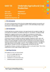
Many processes affect crop performance, but relatively few have a major impact, such as processes resulting in stable efficiency of the use of radiation, water and nutrients for crop growth, those contributing to the water balance and those affecting soil fertility (Bindraban et al., 2000). To describe the land productivity one calculates yield levels that are determined by weather, water and nutrients. Thus, crop production is described in terms of potential, waterlimited and nutrient-limited production. These levels are in fact nested crop production systems starting with the highest or potential production level related to optimal conditions, working down to production levels at sub-optimal conditions (Fig. 2.1).
defining factors: radiation temperature crop characteristics
production situation
potential
limiting factor: water
water-limited
limiting factor: nutrients: N, P
nutrient-limited
reducing factors: weeds pests diseases pollution
actual yield
production (t ha-1) Fig. 2.1: Production situations in hierarchical crop simulation models
11
Chapter 2
2.5.1.
Potential production situation
To obtain the potential production level, crops are grown under conditions of ample supply of water and nutrients, while pest, weed and disease are controlled. Radiation, temperature, CO2 and genetic characteristics of the crop determine the growth rate. Consequently crop growth at this level is predominantly reflected through weather conditions and is determined by the absorbed photosynthetic active radiation only. 2.5.2.
Water-limited production situation
Growth may be limited by shortage of water during at least part of the growing period, even if nutrients are in ample supply. When water supply is insufficient, the soil water content may fall below a threshold and the actual crop transpiration becomes less than potential, resulting in a proportional decrease of crop growth. Next to water stress, crop production can be limited by water excess too. In that case the crop (especially the root system) is encountering oxygen stress, which again can imply a growth reduction. The production level in both cases is the water-limited production. 2.5.3.
Nutrient-limited production situation
Shortage of nitrogen, phosphorous, and/or basic cations occurs in most production systems, often combined with limited water availability. Production situations were nutrients are limiting crop growth are referred to as being nutrient-limited. 2.5.4.
Actual yield
In all three situations, pests, weeds or diseases may further reduce crop yield. The yield measured in the field is referred to as actual yield. The three production levels are used in defining the yield gaps with the actual yield. Yield gaps typically reveal technically feasible options to increase yields (Bindraban et al., 1999). Alternatively, it reflects the extent to which the biological production systems are currently being pushed, realizing that if pushed beyond a biological threshold the systems will likely fail (Bindraban et al., 2000). Modelling crop growth to determine the yield gaps in agricultural production should therefore be seen in its broader
12
From Crop Growth Models to Yield Gap Analysis
context of defining land quality indicators that can guide us towards a sustainable land management (Fig. 2.2).
crop growth modelling
qualitative land evaluation
quantitative land evaluation
sustainable land management
land quality indicators: yield gap analysis
Fig. 2.2: Feedback between crop growth modelling, land evaluation and sustainable land management through yield gap analysis
13
Chapter 3
Radiation-Thermal Production Potential
CHAPTER 3. RADIATION-THERMAL PRODUCTION POTENTIAL
3.1.
Introduction
The radiation-thermal production potential (RPP) is the maximum attainable production of a crop that is optimally supplied with water and nutrients, and grown in absence of pests and diseases. The crop growth model used to determine the RPP is essentially based on the SUCROS model (Penning de Vries and van Laar, 1982). This simple and universal crop growth model simulates the time course of dry matter production of a crop, from emergence till maturity, in dependence of the daily total irradiation and air temperature. The dry matter produced is partitioned over the roots, leaves, stems and storage organs, using partitioning factors that are dependent on the phenological development stage of the crop. This model has been simplified in order to be applicable in most tropical environments, where field trials, offering plant characteristics and responses to be used in the crop growth models, are limited. Further amendments of the calculation procedures and the final evaluation of the results have been performed with reference to the 3-level hierarchical crop growth model used at the Laboratory of Soil Science (Van Ranst, 1994). For the simulation of the RPP, this latter model applies the procedures described by the FAO (1979), as a function of average climatic parameters during the whole crop cycle and only a few crop characteristics cited in literature. This chapter describes and illustrates the elaboration of a new model (Fig. 3.1) describing the most important biochemical processes determining the RPP but without requiring too many crop specific parameters.
15
16
solar radiation, daylength
crop group, day temperature
net daily increase in dry matter (DMI)
net daily assimilation rate (NASS)
daily maintenance respiration rate (MRES)
conversion efficiency
relative respiration rate mean temperature
RESPIRATION
BIOMASS PRODUCTION
daily gross assimilation rate of the canopy under a sky that is partly clear and partly overcast (GASS)
sunshine duration
gross photosynthetic rate of the actually developed canopy under a completely clear (Pcl) and completely overcast sky (Pov)
actual leaf area index
Fig. 3.1: Flowchart of the model estimating the radiation-thermal production potential in Rwanda
16
PHOTOSYNTHESIS
gross photosynthetic rate of a fully developed canopy under a completely clear (PC) and completely overcast sky (PO)
max. photosynthetic rate at light saturation (Amax)
Chapter 3
Radiation-Thermal Production Potential
3.2.
Photosynthesis
In the absence of drought and nutrient shortages, the growth and development of crops are ultimately controlled by the interaction of the plant systems with specific elements of the solar spectrum. Green plants must capture and use external resources, principally light, CO2, water and nutrients, to produce dry matter via photosynthesis. By this process, plants synthesize organic compounds from inorganic materials in the presence of sunlight. Radiation within the visible range is termed photosynthetic active radiation (PAR), as the energy within this waveband is the only radiation that can be actively used by driving pigment-based systems in the process of photosynthesis. The major chemical pathway in photosynthesis is the conversion of atmospheric CO2 and water to carbohydrates and oxygen: CO2 + H2O
CH2O + O2
By the input of solar radiation, two energy-poor compounds are converted into two energy-rich compounds. Photosynthesis is thus a process that reduces atmospheric CO2 and converts light energy into chemical energy. Consequently, a close link exists between the photosynthetic rate and the amount of light that is absorbed. The reduction of CO2 to carbohydrates occurs via two carboxylation pathways: the Calvin cycle and the Hatch-Slack pathway. In C3 crops, the Calvin cycle predominates and the initial fixation product is a three-carbon compound. In C4 crops, the Hatch-Slack pathway predominates and a four-carbon compound is the initial product. Here, CO2 is re-fixed by the Calvin cycle and little or no carbon is lost through photorespiration. The C3 species include all the temperate crops, as well as tropical legumes, root crops and trees, whereas C4 crops include most tropical cereals and grasses (Azam-Ali and Squire, 2002). At any time, the net photosynthetic rate of a green plant depends on (1) the relation between photosynthetic rate and irradiance for each element of the foliage, and (2) on the distribution of the light over the individual elements of the crop foliage (Azam-Ali and Squire, 2002).
17
Chapter 3
3.2.1.
Photosynthesis light response of individual leaves
The typical response of the photosynthetic rate to the irradiance by the individual leaves of a C3 and a C4 crop has been shown in Fig. 3.2. In very weak light, the relation for both C3 and C4 plant systems is almost linear because the photosynthetic rate is limited almost exclusively by the adsorption of light. The initial slope, or initial light use efficiency, is a measure of the amount of CO2 absorbed per unit increase in irradiance. This light use efficiency is about 14.10-9 kg CO2 J-1 absorbed PAR in C4 plants and about 11.10-9 kg CO2 J-1 absorbed PAR in C3 plants. In C3 plants, the light use efficiency increases slightly with CO2 concentration. When light is not limiting, the photosynthesis is controlled by the rate at which CO2 from the atmosphere is reduced to carbohydrate. Pn (g CO2 m-2 h-1) C4 7.5 5.0 C3
2.5
400
800
Irradiance (W m-2)
Fig. 3.2: Typical relationship between photosynthetic rate and irradiance for C3 and C4 species (Azam-Ali and Squire, 2002) After the linear phase, the photosynthetic rate of C3 species in strong light approaches a plateau at a “saturating irradiance” with a maximum value that decreases with leaf age. In contrast, C4 species show less evidence of light saturation and, therefore, no marked plateau in photosynthetic rate at high irradiances. The apparent photosynthetic advantage of C4 crops over C3 crops can thus be ascribed both to the absence of photorespiration and to greater photosynthetic rates in strong light (Azam-Ali and Squire, 2002). This maximum rate of leaf photosynthesis at light saturation varies strongly over the species, with values between 30 and
18
Radiation-Thermal Production Potential
90 kg CO2 ha-1 h-1 for C3 crops and between 15 and 50 kg CO2 ha-1 h-1 for C4 crops (van Keulen and Wolf, 1986). The energy accumulated in the carbohydrates is thus essentially coming from solar radiation. Day temperature, through its effect on the behaviour of enzymes, can influence the reaction speed, although the photosynthetic apparatus of field crops seems to adapt to fluctuating temperatures (van Keulen and Wolf, 1986). Other parameters affecting crop growth are the transpiration rate and the nutrient status of the crop, but when estimating the RPP, these latter conditions are supposed to be non-limiting. Equations that describe the photosynthesis light response curve will thus provide the basic relations for crop growth simulations. There are two equations that are often used. In de Wit (1965), individual leaf photosynthesis exhibits a light response curve of a saturation type, given by the rectangular hyperbola:
A=
A max × ε × I ε × I + A max
where A is the actual photosynthetic rate, Amax the rate of leaf photosynthesis at light saturation, I the absorbed photosynthetic active radiation and ε the initial light use efficiency. The maximum photosynthetic rate at light saturation was taken as 0.8 × 10⁻⁶ kg CO2 m-2 s-1, the efficiency of light use at low light intensity was 21 × 10-9 kg CO2 J-1. This rectangular hyperbola thus resulted in a rather slow and gradual approach of photosynthesis to the saturation level with increasing light intensity. Later measurements (van Laar and Penning de Vries, 1972) indicated that this approach is too slow and that a better fit can be obtained with an asymptotic equation such as:
I × ε A = A max × 1 − exp − A max This equation is more linear at low light than the hyperbolic one. Therefore, even though the initial slope is less, it crosses over at a higher light intensity. In this case the initial light use
19
Chapter 3
efficiency is 14× 10-9 kg CO2 J-1, while the maximum photosynthetic rate at light saturation remains 0.8 × 10⁻⁶ kg CO2 m-2 s-1. The evolution of the photosynthetic rate with irradiation according to both equations is shown in Fig. 3.3. 0.8
gross photosynthesis (10-6 kg CO 2 m-2 s-1)
0.7 0.6 0.5 0.4 0.3 0.2 De Wit (1965) Goudriaan (1977)
0.1 0.0 0
20
40
60
80
100
absorbed PAR (W/m²)
Fig. 3.3: Photosynthesis-light response curve of individual leaves according to De Wit (1965) and Goudriaan (1977) 3.2.2.
Distribution of light through the canopy
For a crop to produce dry matter, his leaves must intercept radiation and absorb CO2. The size and duration of the crop foliage determine the rate and duration of dry matter accumulation. The size of the intercepting surface depends on the green leaf area index of a crop. The amount of light that penetrates the canopy and strikes the ground depends both on environmental characteristics, such as the solar radiation and the solar height, and on crop canopy characteristics such as the leaf area index and the angular arrangement of the individual leaves. To describe the pattern of light penetration through a crop canopy, it is convenient to imagine a crop as consisting of a number of horizontal layers each with a leaf area index of 1.
20
Radiation-Thermal Production Potential
If radiation is measured at a number of levels down the crop profile, then the measured irradiance at any level is a function of the angular arrangement of the leaves above that level. The relationship for the extinction of light down a crop canopy is often described by the MonsiSaeki (1953) equation:
I p = I 0p × e − k×L where I p is the (penetrating) irradiance at a level within the canopy below a leaf area index of
L, I 0p is the irradiance above the canopy, and k is an extinction coefficient for radiation (Fig. 3.4).
Fig. 3.4: Exponential decay of radiation through a crop stand (Azam-Ali and Squire, 2002)
The fraction of intercepted (adsorbed) radiation at each level in the crop canopy,
Ia I 0p
, thus can
be derived from the Monsi-Saeki adsorption function (1953): I a = I 0p − I p
⇒
I a = I 0p − I 0p × e − k×L ⇒
Ia I 0p
= 1 − e − k ×L
21
Chapter 3
However, it should be noted that the Monsi-Saeki equation assumes that the canopy is a homogeneous medium whose leaves are randomly distributed. In these circumstances, light transmission obeys Beer’s law of exponential decay. Strictly, for attenuation to be exponential, the leaves should be black, i.e. opaque to radiation (Azam-Ali and Squire, 2002). Instead of being opaque to radiation, in reality, leaves are reflecting, absorbing and transmitting the incoming radiation, resulting in a multiple scattering of the light in the crop canopy. Averaged over the wavelength bands the scattering coefficient of green leaves is about 0.2 for visible radiation. In case that (1) the leaf transmission and reflection coefficients are each equal to half the scattering coefficient, (2) the sub-layers are infinitesimally small and (3) the leaves are horizontal, then the reflection coefficient of the canopy can be estimated by:
ςc =
1− k 1+ k
where ς c is the reflection coefficient and k the extinction coefficient. For a spherical leaf angle distribution, the extinction coefficient is approximately equal to k = 0 .8 × 1 − σ for diffuse light, and
k=
0.5 × 1 − σ sin β
for direct light, with σ the scattering coefficient and b the solar height, which changes during the day. Consequently, when the sun shines, the fraction of diffuse and direct radiation should be known, together with the fraction of sunlit and shaded leaf area. The sunlit leaves must be classified according to the angle of incidence of the direct light on the leaf, and most of them will photosynthesise at the light saturation level (Penning de Vries and van Laar, 1982). Goudriaan (1977) has shown Beer’s law to be a good approximation in many real canopies, with an extinction coefficient depending on the architecture of the crop. Crops with narrow, erect
22
Radiation-Thermal Production Potential
leaves tend to have lower values of k than crops with more horizontally displayed leaf arrangements. Beans, for instance, have an extinction coefficient of about 0.80, while for sorghum this is only 0.46. Maize has an intermediate extinction coefficient of about 0.65 (Lemeur, 1994). When the extinction coefficient is known, the fraction of radiation intercepted by a crop can be calculated from knowledge of the leaf area index (LAI), reckoned from the top of the canopy: f = 1 − e − k×LAI Experimental studies indicate that the final extinction of the light in the crop, not only varies with the canopy characteristics, but also with the solar height, row spacing, row direction and latitude (Thornley, 1976). In the SUCROS model (Goudriaan and van Laar, 1978), an average extinction coefficient of 0.8 is assumed, which holds for a spherical leaf angle distribution. 3.2.3.
Gross assimilation
“Gross” assimilation should be used when referring to the products of the photosynthesis process, and will be governed by the interaction between incoming radiation, crop photosynthetic capability (photosynthesis light response curve), leaf area, leaf architecture and crop cycle length. The effect of this last parameter should not be underestimated. The longer the crops are on the field, the longer they can produce and accumulate dry matter. Modelling daily gross assimilation
De Wit (1965) calculated the gross dry matter production of a leaf canopy, based on the photosynthesis-light response curve for individual leaves and a set of standard conditions. His results were tabulated and have been used by the FAO model (FAO, 1979) to estimate the gross photosynthesis rate of a fully developed canopy at a particular time and place on earth. In Goudriaan and van Laar (1978), however, de Wit’s method has been discussed in detail and some revisions have been proposed. Goudriaan (1977) simulated the instantaneous photosynthesis rate following the rectangular hyperbola photosynthesis-light response curve of individual leaves. The simulation was done for different values of maximum photosynthesis rate at light saturation. The initial light use
23
Chapter 3
efficiency was taken at 14 × 10-9 kg CO2 J-1. The leaf area index was taken at 5, so that the canopy was practically closed. The spatial distribution of the leaves was set to be spherical, and the solar height determined the incoming PAR over the daylength. In this schematised set up, two situations were considered: a completely overcast and a completely clear sky. The incoming radiation under the overcast sky was set to 20 % of that under the clear sky (Goudriaan and van Laar, 1978). The amount of diffuse and direct irradiation, and the fraction of sunlit and shaded leaves, had to be modelled. In each leaf sub-layer, the fraction of sunlit leaf area is equal to the overall fraction of the direct irradiation that reaches that level. Therefore, when the LAI was large enough, the total sunlit leaf area was set to: 1 − e − k dir ×LAI 1 ≈ k dir k dir with kdir being the extinction coefficient for direct sunlight. For a spherical leaf angle distribution, kdir equals 0.5/sinβ, so that the sunlit leaf area was set equal to 2 × sinβ. For each leaf sub-layer (LAI = 1), the instantaneous photosynthesis rate was calculated based on balance of the incoming and outgoing radiation fluxes (Fig. 3.5). The extinction of light in the canopy was exponential with the leaf area index reckoned from the top. The effect of multiple scattering was accounted for by introducing a scattering coefficient of 0.2 in the equations for the extinction and reflection coefficient, as has been discussed above (Penning de Vries and van Laar, 1982).
direct incoming S1 reflection S5 = ρ x S1
reflection S4 = ρ x S2 direct downward flux S3
top 1 leaf layer bottom total downward flux S2 direct + diffuse (scattering)
Fig. 3.5: Different fluxes of direct incoming radiation in a leaf layer (Penning de Vries and van Laar, 1982)
24
Radiation-Thermal Production Potential
Finally, integration of the instantaneous rates of radiation flux and assimilation yielded the daily amount of CO2 fixed. The daily gross assimilation rates for maximum rates of photosynthesis of a single leaf at high light intensity have been tabulated as a function of latitude. Values are available for the middle of each month and for completely clear and overcast skies, under the assumption of zero dark respiration and a LAI of 5. These results are shown in Table 3.1 and Table 3.2. Interpolation techniques can be used to find the gross photosynthesis rate of a crop grown at specific latitude and on a specific day of the year. Estimating daily gross assimilation
In order to avoid the use of tables, which are cumbersome to handle, Goudriaan and van Laar (1978) developed some descriptive equations based on the process itself. Descriptive equations can be used to calculate the gross CO2 assimilation of leaf canopies for each day of the year. Regression of the estimated gross assimilation rates to the tabulated rates finally results in a best estimate for the gross CO2 assimilation of leaf canopies for each day of the year and at all latitudes. These descriptive equations have been introduced in a new crop simulation model that is capable of simulating the daily course of the crop dry matter production without increasing the required information on crop characteristics. This model will be further referred to as the DAIly CROp Simulation model (DAICROS). Its performance will be evaluated through a comparison of the intermediary and final results with those of the crop growth model described by the FAO (1979), further referred to as FAOCROS.
25
26
26
70
60
50
40
30
20
10
0
(°N)
latitude
0
0
PO
15
PO
PC
71
64
PO
PC
227
122
PO
PC
389
180
PO
PC
543
234
PO
PC
680
282
PO
PC
796
321
PO
PC
894
PC
15/jan
10
47
58
212
116
377
174
529
227
663
272
773
309
859
336
926
15/feb
74
268
135
437
193
584
242
707
283
803
314
873
335
920
345
946
15/mar
193
615
244
733
286
829
318
898
340
942
351
963
351
960
341
937
15/apr
311
948
336
980
358
1014
372
1033
376
1032
369
1010
353
967
327
906
15/may
381
1151
383
1107
393
1104
396
1095
390
1070
375
1027
350
964
316
883
15/jun
353
1066
365
1057
379
1069
387
1071
385
1056
373
1021
352
966
321
892
15/jul
247
766
287
850
320
918
344
964
358
987
361
988
353
966
335
925
15/aug
120
403
180
558
232
688
275
790
309
865
332
915
344
941
345
947
15/sep
gross daily canopy photosynthetic rate (kg CO2 ha-1d-1)
clear (PC) sky conditions (Goudriaan and van Laar, 1978)
28
119
84
289
144
451
199
595
248
716
289
812
320
884
341
937
15/oct
0
0
25
107
78
266
137
427
194
576
245
707
290
815
326
904
15/nov
0
0
8
40
52
192
109
354
168
511
224
654
274
777
316
883
15/dec
Table 3.1: Gross daily canopy photosynthetic rate for a C4 crop with an Amax of 60 kg CO2 ha-1h-1 and a LAI of 5 under overcast (PO) and
Chapter 3
27
70
60
50
40
30
20
10
0
(°N)
latitude
0
0
PO
15
PO
PC
66
63
PO
PC
183
117
PO
PC
294
169
PO
PC
396
217
PO
PC
486
259
PO
PC
560
293
PO
PC
623
PC
15/jan
10
45
57
175
112
288
164
389
211
475
250
545
282
600
305
642
15/feb
72
220
130
333
181
429
225
507
260
566
286
610
304
638
312
654
15/mar
184
467
229
536
265
593
292
633
309
657
318
668
318
664
309
648
15/apr
293
699
312
704
329
716
339
721
341
716
334
699
320
670
297
630
15/may
357
846
354
790
359
776
360
763
353
742
340
711
318
669
289
616
15/jun
331
784
338
756
348
753
352
747
349
732
338
707
319
670
292
622
15/jul
234
572
268
615
296
652
315
676
325
686
327
684
320
669
304
641
15/aug
116
318
170
417
217
499
254
562
282
607
301
637
311
652
312
654
15/sep
gross daily canopy photosynthetic rate (kg CO2 ha-1d-1)
clear (PC) sky conditions (Goudriaan and van Laar, 1978)
27
109
81
230
137
339
187
433
230
510
264
570
291
616
309
648
15/oct
0
0
25
98
76
211
130
321
181
419
227
503
266
572
297
629
15/nov
27
0
0
8
38
51
158
105
270
159
375
208
469
252
549
289
616
15/dec
Table 3.2: Gross daily canopy photosynthetic rate for a C3 crop with an Amax of 30 kg CO2 ha-1h-1 and a LAI of 5 under overcast (PO) and
Radiation-Thermal Production Potential
Chapter 3
3.2.4.
Calculation of astronomical parameters
Before proceeding to the elaboration of the descriptive equations, an overview of the equations describing the most important astronomical parameters affecting photosynthesis has been presented below. Daylength
The following equations were applied to calculate the astronomical daylength: N = 43200 × with N
{π + 2 × arcsin(s sin c cos )} π
= astronomical daylength [s d-1]
ssin
= sin δ sin λ [−]
ccos
= cos δ cos λ [−]
λ
= latitude [rad]
δ
= solar declination [rad]
The effective daylength, that part of the day that the crop is effectively photosynthesising, is shorter than the astronomical daylength and was found to be best estimated as the duration of the time that the solar height exceeds 8°: N eff = 43200 × with Neff
{π + 2 × arcsin((− sin (8) + s sin ) c cos )}
= effective daylength [s d-1]
ssin
= sin δ sin λ [−]
ccos
= cos δ cos λ [−]
λ
= latitude [rad]
δ
= solar declination [rad]
The solar declination has been estimated by:
28
π
Radiation-Thermal Production Potential
day + 10 365
δ = −0.409 × cos 2 × π ×
with day
= number of the day in the year
Solar radiation
The solar radiation under a clear sky depends on the solar height, which is changing with latitude, solar declination and solar time. The calculation of the average daily incoming radiation, for all latitudes and for each day of the year, has been performed according to the following equations (Penning de Vries and van Laar, 1982):
R so = 1280 × int sin β × e with Rso
−0.1
int sin β N
= average daily solar radiation under a clear sky [J m-2 d-1]
intsinβ
= average daily solar height [s d-1]
N
= astronomical daylength [s d-1]
0.1
= extinction of radiation in a very clear atmosphere [-]
The average daily solar height has been given by integrating the solar height over the day:
int sin β = sin λ sin δ * N +
with intsinβ
86400
π
sin λ sin δ * cos λ cos δ × 1 − cos λ cos δ
2
= average daily solar height [s d-1]
λ
= latitude [rad]
δ
= solar declination [rad]
N
= astronomical daylength [s d-1]
Photosynthetic active radiation
The daily solar radiation consists for 50 % of photosynthetic active radiation (PAR). The average daily PAR under an overcast sky amounts to 20 % of that under a clear sky. These
29
Chapter 3
average daily values should be divided through the effective daylength to find the incoming PAR expressed in J m-2 s-1 or, RADO =
with RADO
3.2.5.
0.2 × 0.5 × R so N eff
= average daily PAR under an overcast sky [J m-2 s-1]
Rso
= average daily solar radiation under a clear sky [J m-2 d-1]
Neff
= effective day length [s d-1]
Gross photosynthetic rate of a fully developed canopy
Crop photosynthesis, just like individual leaf photosynthesis, exhibits a light response curve of a saturation type. The actual crop photosynthesis amounts to a fraction of the saturation level, which can be represented by a rectangular hyperbola. This general idea has been applied to estimate the daily gross photosynthesis of a fully developed canopy under a completely overcast sky or a completely clear sky. The leaf angle distribution was assumed to be spherical, and leaf area index was set to 5. A linear regression was made between the model results and the results for the descriptive equations. As such, the best estimates for the model results could be calculated. For low values of LAI, the photosynthesis rate was reduced, according to the fraction of light intercepted. An additional procedure has been developed to set an upper limit to the rate of photosynthesis, especially for low rates of maximum photosynthesis at light saturation. Although crop photosynthesis under an overcast or clear sky is following the same principles, important differences between the two cannot be neglected. The sunlit and shaded leaves will contribute in a different way to total photosynthesis than the leaves intercepting only diffuse radiation under an overcast sky. The more unequal light distribution under a clear sky than under an overcast sky is reflected in different formulae and consequently the two cases will be discussed separately.
30
Radiation-Thermal Production Potential
Gross daily canopy photosynthesis under an overcast sky Daily gross crop photosynthesis of a closed canopy under an overcast sky is given by:
PO f = P × A max × LAI × N eff = daily gross photosynthetic rate of a closed canopy under an overcast sky
with POf
[kg CO2 m-2d-1]
The
P
= fraction of the daily canopy photosynthetic rate at light saturation [-]
Amax
= leaf photosynthetic rate at light saturation [kg CO2 m-2 (leaf) s-1]
LAI
= leaf area index = 5 [m² (leaf) m-2]
Neff
= effective daylength
photosynthetic
0.84 × 10
-6
rate
of
-2
-1
kg CO2 m
s
an
[s d-1]
individual
leaf
at
light
saturation
amounts
to
for a C3 crop (i.e. groundnut, bean, potato) and
1.67 × 10⁻⁶ kg CO2 m-2 s-1 for a C4 crop (i.e. sorghum, maize). This value should be multiplied with the leaf area index to find the photosynthetic rate at light saturation for the complete canopy. Initially, a leaf area index of 5 is supposed, corresponding to a completely closed canopy. The resulting photosynthetic rate is expressed in kg CO2 m-2 s-1. Multiplying Amax, LAI and Neff gives the daily, maximum, gross photosynthetic rate at light saturation of a fully developed canopy with a leaf area index of 5. The actual daily gross canopy photosynthetic rate however, is a fraction P of the maximum photosynthetic rate at light saturation. The fraction P is given by: P=
X X +1
with
X=
and
RADO × EFFE A max × LAI
RADO
= average daily incoming PAR on an overcast day [J m-2 s-1]
EFFE
= canopy light use efficiency for the incoming PAR kg CO2 J-1]
Amax
= leaf photosynthetic rate at light saturation [kg CO2 m-2 (leaf) s-1]
31
Chapter 3
LAI
= leaf area index = 5 m² (leaf) m-2]
The denominator corresponds to the maximum gross photosynthetic rate at light saturation. The numerator corresponds to the gross photosynthetic rate, which follows from the incoming PAR and the light use efficiency at low light intensities. From the photosynthesis-light response curves for individual leaves, it is found that the light use efficiency for the incoming PAR is 14 × 10-9 kg CO2 J-1. Since about 8 % of the PAR is reflected by a closed canopy, an efficiency of 12.9 × 10⁻⁹ kg CO2 J-1 is used for EFFE. A linear regression between the model results and the results of the descriptive equations yields the best estimates for the model results. For the photosynthetic rate under an overcast sky, the following linear regression equation has been applied:
PO m = 0.9935 × PO f + 0.11 × 10 −3 with POm
= best estimate for the daily photosynthetic rate of a fully developed canopy under an overcast sky [kg CO2 m-2d-1]
POf
= daily photosynthetic rate of a fully developed canopy under an overcast sky, calculated with the descriptive equations [kg CO2 m-2d-1]
Gross daily canopy photosynthesis under a clear sky
The daily gross crop photosynthetic of a closed canopy under a clear sky [kg CO2 m-2d-1] is given by:
PC f = PS + PSH with PS PSH
= daily gross canopy photosynthetic rate of sunlit leaves [kg CO2 m-2d-1] = daily gross canopy photosynthetic rate of shaded leaves [kg CO2 m-2d-1]
Thus, two classes of leaves are distinguished, sunlit and shaded. For a spherical leaf angle distribution, the sunlit area is given by 2 × sin(β) where β is the actual solar height. As a rough estimate, the average sine of the solar height is half of that at noon. Thus, the average daily sunlit leaf area can be estimated as the sine of the solar height angle at noon.
32
Radiation-Thermal Production Potential
SLLAE = sin ( with SLLAE
π + δ − λ) 2
= average daily sunlit leaf area [m² (leaf) m-²]
δ
= solar declination [rad]
λ
= latitude [rad]
The gross daily canopy synthesis of the sunlit leaves is then:
PS = Ps × A max × SLLAE × N eff with PS
= gross daily canopy photosynthetic rate of sunlit leaves [kg CO2 m-2d-1]
Ps
= fraction of maximum photosynthetic rate for sunlit leaves [-]
Amax
= maximum photosynthetic rate at light saturation [kg CO2 m-2 s-1]
SLLAE
= sunlit leaf area [m² (leaf) m-2]
LAI
= leaf area index = 5 [m² (leaf) m-2]
Neff
= effective daylength [s d-1]
And the gross photosynthetic rate of the shaded leaves is then:
PSH = Psh × A MAX × (LAI − SLLAE) × N eff with PSH
= gross daily canopy photosynthetic rate of shaded leaves [kg CO2 m-2d-1]
Psh
= fraction of maximum photosynthetic rate for shaded leaves [-]
Amax
= maximum photosynthetic rate at light saturation [kg CO2 m-2 s-1]
SLLAE
= sunlit leaf area [m² (leaf) m-2]
LAI
= leaf area index = 5 [m² (leaf) m-2]
Neff
= effective daylength
[s d-1]
By searching the best fit, it was found that 45% of the incoming PAR is allotted to the average sunlit leaf area. Consequently,
Xs =
0.45 × RADC × EFFE SLLAE × A max
and
33
Chapter 3
X sh =
with Xs
0.55 × RADC × EFFE
(LAI − SLLAE) × A max
= variable X for sunlit leaves [-]
Xsh
= variable X for shaded leaves [-]
RADC
= incoming PAR under clear sky [J m-2 s-1]
EFFE
= initial light use efficiency [kg CO2 J-1]
SLLAE
= sunlit leaf area [m² (leaf) m-2]
LAI
= leaf area index = 5 [m² (leaf) m-2]
Amax
= maximum photosynthesis rate at light saturation [kg CO2 m-2 s-1]
A second effect of the unequal light distribution is that the saturation level is approached more gradually than under an overcast sky. Such a phenomenon can be represented by replacing the dimensionless variable X by ln(1+X) before substitution into the rectangular hyperbola. The equations are now given by: X s' = ln (1 + X) and Ps =
X s' 1 + X s'
' X sh = ln (1 + X) and Psh =
' X sh ' 1 + X sh
The best estimates for the gross photosynthetic rate under a clear sky are found by applying the following linear regression equation: PC m = 0.95 × PC f + 2.05 × 10 −3 with PC
= best estimate for the daily photosynthetic rate of a fully developed canopy under a clear sky [kg CO2 m-2d-1]
PCf
= daily photosynthetic rate of a fully developed canopy under a clear sky, calculated with the descriptive equations [kg CO2 m-2d-1]
34
Radiation-Thermal Production Potential
3.2.6.
Gross photosynthetic rate of a non-closed crop surface
For low values of the LAI, when the canopy does not form a closed crop surface, radiation is lost to the soil and photosynthesis is reduced. This reduction can be estimated by the fraction of intercepted radiation: f int = 1 − exp ( − k × LAI) with fint
= fraction of intercepted radiation when the LAI < 5 [-]
LAI
= actual leaf area index [m² (leaf) m-2]
k
= extinction coefficient = 0.5 [-]
In many tropical systems, crops rarely, if ever, cover the ground completely. This can be because crops are deliberately sown in distinct clumps or rows, to optimise the use of available water rather than light. In these circumstances, the Beer’s law analogy of randomly distributed leaves and the corresponding Monsi-Saeki equation fails (Azam-Ali and Squire, 2002). However, several authors (Begg et al., 1964; Bonhomme et al., 1982; Muchow et al., 1982) used extinction coefficients of about 0.4 and 0.6 in tropical areas characterised by a higher average solar height and wider row spacing. The influence of the crop architecture and solar height on gross assimilation is especially important when simulating crop growth with an hourly temporal resolution. For daily models, a constant extinction coefficient suffices. Instead of using the extinction coefficient of 0.8, used in the SUCROS model (Goudriaan and van Laar, 1978), an average extinction coefficient for crop stands in the tropics of 0.5 has been taken into account. For low values of Amax, photosynthesis is better related to leaf area than to intercepted radiation. In the extreme situation, all leaves are photosynthesising at the maximal rate all day long. In that case the daily photosynthesis rate is given by Amax × LAI × N. In fact, both estimates fint × POm (C1) and Amax × LAI × N (C2), give an upper limit to the rate of photosynthesis. When these estimates are not much different, it means that saturation with light gives a considerable reduction and that photosynthesis is less than predicted by fint × POm. The best estimation for the canopy gross photosynthesis rate on overcast days (Pov) is obtained by applying the following rules:
35
Chapter 3
If C1 is greater than C2 then C − 1 C2 Pov = C 2 × 1 − e
C − 2 Pov = C1 × 1 − e C1
If C1 is smaller than C2 then
with Pov
= daily photosynthetic rate of the canopy under a completely overcast sky [kg CO2 m-2d-1]
C1
= fint × POm [kg CO2 m-2d-1]
C2
= AMAX × LAI × N [kg CO2 m-2d-1]
The same procedure can be applied for the daily photosynthetic rate of the canopy under clear sky conditions, Pcl. 3.2.7.
Actual gross canopy assimilation rate
The previous procedure yields the daily photosynthetic rate of the canopy under a completely clear or an overcast sky. The actual hours of sunshine can be used to determine the fraction of the day that the sky is overcast or clear. The actual daily gross assimilation rate is calculated as the sum of the photosynthetic rate during the clear sky period and that during the overcast period: GASS' = f × Pov + (1 − f) × Pcl with GASS’
36
= actual daily gross assimilation rate [kg CO2 m-2d-1]
Pov
= daily photosynthetic rate under an overcast sky [kg CO2 m-2d-1]
Pcl
= daily photosynthetic rate under a clear sky [kg CO2 m-2d-1]
f
= fraction of the day that the sky is overcast [-]
1-f
= fraction of the day that the sky is clear [-]
Radiation-Thermal Production Potential
and f =1− with n N
n N
= actual hours of sunshine [h] = astronomical daylength [h] = maximum possible hours of sunshine
The absorbed CO2 is reduced in the crop to carbohydrates or sugars. To express the assimilation rate expressed in CH2O, the rate in CO2 is multiplied by
30 , the ratio of their molecular 44
weights. The gross assimilation rate can be further converted to assimilates per hectare instead of per square meter. GASS = 10 4 × with GASS GASS’
30 × GASS' 44
= actual daily gross assimilation rate [kg CH2O ha-1d-1] = actual daily gross assimilation rate [kg CO2 m-2d-1]
37
Chapter 3
3.3.
Respiration
The net dry matter increase, however, is not only determined by the photosynthesis rate. Losses due to respiration should be included too. High-energy compounds are broken down through two pathways: photorespiration and dark respiration. The process of photorespiration is induced in C3 plants by the presence of oxygen. Photorespiration acts on the CO2 initially fixed by photosynthesis and its rate is therefore closely linked to the CO2 fixation rate. The importance of photorespiration increases with temperature, resulting in a reduction of the initial efficiency of light use of individual leaves. Photorespiration of C3 crops has already been accounted for by a lower photosynthetic rate at light saturation. There is no photorespiration in C4 plants. Irrespective of their photosynthetic system, all green plants undergo the process of dark respiration in which atmospheric oxygen is used by plants to convert carbohydrates into CO2
and water, with the simultaneous liberation of energy. Plants use this energy to build more complex molecules from the initial products of photosynthesis. Respiration is an important part of the carbon budget of crops because it is responsible for the loss of CO2 from plant cells. It can be considered at two levels: (1) that, which occurs as a result of the growth of crops and (2) that, which is required for their maintenance. It is generally assumed that, at any given temperature, respiration continues in the light at a comparable rate to that of the dark. Moreover, during the life of a crop, the relative contributions of the growth and maintenance components of respiration change with the age and weight of the crop (Azam-Ali and Squire, 2002). 3.3.1.
Maintenance respiration
Maintenance processes in plants consist of re-synthesis of degraded proteins and maintenance of ion gradients across cell membranes. Both processes require a constant supply of energy, delivered by the maintenance respiration process (Penning de Vries and van Laar, 1982). Although accurate data on maintenance requirements are scarce, reasonable estimates can be made on the basis of the composition of the biomass present. As the maintenance process is mainly related to protein content, its calculation can be based on the protein content of the tissue. In the SUCROS model, the relative maintenance respiration rate of the different plant
38
Radiation-Thermal Production Potential
organs has been estimated based on their composition. As such, for each organ, the gross assimilation rate and the maintenance respiration rate could be estimated. In the DAICROS model, the partitioning of dry matter production hasn’t been included, and therefore, the maintenance respiration rate should be estimated at the level of the total crop. Estimates of the relative maintenance respiration rate, Rm, at a standard temperature of 20°C are given in Table 3.3 for four groups of crops; each group having approximately the same chemical composition (van Keulen and Wolf, 1986). Table 3.3: Relative maintenance respiration rate and conversion efficiency of different crop groups (van Keulen and Wolf, 1986) crop group
relative maintenance respiration rate -1
-1
conversion efficiency
(kg CH20 kg CH20 d )
(kg DM kg-1CH20)
root and tuber crops
0.010
0.75
cereals
0.015
0.70
protein-rich seed crops
0.025
0.65
oil-rich seed crops
0.030
0.50
Effects of the environment on the intensity of the process are not so well established. Temperature, the most important factor, usually stimulates the maintenance process by a factor of 2.0 per 10 °C temperature increase (van Keulen and Wolf, 1986). A light water stress does probably not affect the intensity of the maintenance process. In order to take into account the impact of temperature, the maintenance respiration has been calculated as follows:
MRES = R m × TDW × Q10 with MRES
(t mean − 20) 10
= daily maintenance respiration rate [kg(CH2O) ha-1 d-1]
Rm
= relative maintenance respiration rate at 20 °C [kg(CH2O) kg-1(DW) d-1]
TDW
= total accumulated dry weight [kg(DW) ha-1]
Q10
= 2 [-]
tmean
= mean daily temperature [°C]
39
Chapter 3
3.3.2.
Growth respiration
The amount of assimilation products available for increase in dry weight of the crop equals the difference between the gross assimilation and the maintenance respiration. The conversion of the primary photosynthates into structural materials (carbohydrates, proteins, lipids, lignin, organic acids, minerals) requires substrate for building materials and energy for synthesis of the product, the transport of sugars and the uptake of nitrogen and minerals. Therefore, part of the sugars assimilated is respired to provide energy for the synthesis of new plant components. Another part is lost as refuse in the process of synthesis. Different biochemical pathways, characterised by different weight efficiencies, are employed for conversion of reserves into each of these components. The magnitude of the growth respiration is thus determined by the composition of the end product formed. Fats and lignin are produced at high costs, structural carbohydrates and organic acids are relatively cheap. Proteins and nucleic acids form an intermediate group (Penning de Vries and van Laar, 1982; van Keulen and Wolf, 1986). The growth respiration can also be represented by its complement, the conversion efficiency Eg. Consequently, the dry weight increment is equal to the conversion efficiency times the available assimilation products. In the SUCROS model, average conversion factors have been used for leaf, stem, root, and grain biomass (Penning de Vries and van Laar, 1982). The DAICROS model uses conversion efficiencies of different crop groups as has been tabulated in Table 3.3. At high temperatures, the rate of conversion of primary photosynthates into structural plant material changes, but the conversion efficiency remains constant, because the biochemical pathway is not affected by temperature. However, as the conversion occurs largely at night, low night temperatures may hamper the process. 3.3.3.
Net assimilation
The daily dry matter increase is then given by: DMI = E g × NASS = E g × (GASS − MRES) with DMI Eg
40
= daily dry matter increase [kg(DW) ha-1 d-1] = conversion efficiency [kg(DW) kg-1(CH2O)]
Radiation-Thermal Production Potential
NASS
= net assimilation rate [kg(CH2O) ha-1 d-1]
GASS
= gross assimilation rate [kg(CH2O) ha-1 d-1]
MRES
= maintenance respiration rate [kg(CH2O) ha-1 d-1]
If, at the end of the crop cycle, the maintenance costs are higher than the daily dry matter increase, the net assimilation rate is set to 0. Destruction of the produced biomass is thus not allowed to occur. Summation of the daily dry matter increase over the crop cycle gives the total dry weight of the crop at harvest.
41
Chapter 3
3.4. Yield efficiency For many determinate crops, the reproductive weight of individual plants is closely related to the total dry weight of each plant above a minimum weight of vegetative infrastructure necessary before reproductive growth can commence. The ratio of reproductive or economic yield to total dry weight, indicated as the harvest index, remains constant. However, the allocation of assimilates to the reproductive or economically important components, is not always conservative and estimates of yield based on such an assumption may be very wrong. This is particularly the case for crops that are grown in marginal areas, relying on stored soil water. Here, the vegetative phase may continue more-or-less as normal whilst there is adequate water but drought will become increasingly important during grain filling. This will lead to premature senescence of leaves and a reduction in crop photosynthetic potential. The net effect will be a crop with a reasonable vegetative growth but poor final yield (Azam-Ali and Squire, 2002). When calculating the economic yield at the RPP level however, water and nutrient supply are considered to be optimal. Some harvest indices of crops grown in similar optimal conditions are given in Table 3.4. Table 3.4: Harvest index of some crops grown in Rwanda (Sys et al., 1993) crop
harvest index (-)
potato
0.60
common bean
0.30
groundnut
0.30
maize
0.35
sorghum
0.25
The total accumulated crop biomass at harvest includes all above- and underground plant organs. In the DAICROS model, multiplication of the net accumulated biomass with the harvest index gives the yield (t ha-1) of the economically useful part of the crop. This approach is similar to the one followed by the FAOCROS model (1979).
42
Radiation-Thermal Production Potential
3.5. Crop development 3.5.1.
Phenological stages
With respect to the growth rate, three phases may be distinguished (Fig. 3.6). During the first phase the crop consists of individual plants that do not shade each other and the growth rate increases. In the second phase the crop covers the soil completely and the growth rate is constant. In the third phase the crop is maturing and the growth rate is decreasing.
Fig. 3.6: Schematised course of growth rate and total dry weight (Azam-Ali and Squire, 2002)
In the first phase, most assimilates are invested in leaf growth. This increase in leaf area is accompanied by a proportional increase in energy interception, because neighbouring plants are so small that mutual shading hardly plays a role. Individual plant weight increases by a constant proportion per day, thus leading to exponential growth. After a closed crop surface has been formed, more leaf growth does not lead to more light interception, hence the growth rate remains constant and total plant weight increases linearly. In the last phase, leaf senescence leads to a decrease in the growth rate. The major part of the total dry matter accumulation is achieved during the second phase. Total dry matter production of the crop is thus largely determined by the magnitude of the growth rate during the linear phase and the duration of that phase (van Keulen and Wolf, 1986).
43
Chapter 3
However, a crop not only accumulates weight, it also passes through successive phenological development stages, characterised by the order and rate of appearance of vegetative and reproductive organs. The order of appearance of the various organs is a species-specific. It may vary among species and is almost independent of the circumstances (Van Keulen and Wolf, 1986). Timing and rate of organ appearance, however, is dependent on genetic and environmental conditions and is, consequently, highly variable. The major environmental conditions influencing phenological development are temperature and daylength. Winter crops need a period of low temperature to induce flowering. This process is called vernalisation. Summer crops in temperate and tropical climates do not need a period of low temperature. For all crops however, higher temperatures shorten the length of a given phenological stage. The shape of the curves relating the number of days until anthesis to temperature suggests a constant product of days and temperature. This product is the temperature sum or so called thermal unit (TU). The most common method of obtaining TU values for the duration of a phenological stage is to add average daily temperatures above a threshold value. The range of threshold values varies between 0 and 10 °C for different crops, species and varieties. Consequently, the development rate increases and the length of the total growing period decreases with increasing temperature. For a discussion on the bases and limits of using these “degree.day” units to determine crop development, the reader is referred to a review written by Bonhomme (2000). For some species, the effect of temperature on development is modified by the influence of the length of the day, or, in fact, the length of the dark period. This effect is called photoperiodism. With regard to this mechanism, plants may be classified into three groups: (1) day-neutral plants, for which development rate is insensitive to daylength; (2) long-day plants, for which anthesis is induced by the occurrence of long days; and (3) short-day plants, for which anthesis is induced by the occurrence of short days. The reaction to daylength may be an important characteristic when a new species or cultivar is introduced in a region. In the SUCROS model (Penning de Vries and van Laar, 1982), the phenological stage of the canopy is characterised by its development stage, a variable having the value 0 at emergence, 1 at flowering and 2 at maturity. Intermediate values are obtained by the integration of the rate of development, which depends on the average daily temperature and the daylength in the vegetative phase, and on temperature only afterwards. Differences in temperature sensitivity
44
Radiation-Thermal Production Potential
between species and cultivars may exist, associated with photoperiodic influences. The impact of temperature and daylength on the development rate is crop-, species-, and cultivar-specific, and thus it needs to be established experimentally. Often, these data are not available to the land evaluators. The DAICROS model should therefore be applicable with only local data on the length of the total crop cycle and literature data on the relative length of the crop development stages. Four phenological development stages have been distinguished: •
initiation
: from germination to early growth
•
crop development
: from early growth to effective full ground cover
•
mid-season
: from effective full ground cover to start of maturation
•
late-season
: from the start of maturation to full maturity or harvest
Early growth is characterised by a ground cover percentage less than 10, while effective full ground cover is reached at 70 to 80 %. The discolouring or shedding of the leaves marks the beginning of maturation (Sys et al., 1991a). The agricultural calendar of the lowlands, middle altitudes and highlands, as described by Ndayizigiye (1993) has been used to derive the crop cycle length of the most important crops cultivated in Rwanda. These cycle lengths were then compared with the standard lengths of the different crop growth stages, described in Sys et al. (1993), to give a sound estimation of the length of the different development stages of crops grown in the three different altitudinal regions of Rwanda. The results are shown in Table 3.5. The effects of daylength have not been treated quantitatively, because it is assumed that in each region species with the proper daylength reaction are cultivated. 3.5.2.
Partitioning of assimilates and leaf growth
Although the basic processes governing phenological development and biomass production act independently, both phenomena are strongly interrelated. If the rate of development is high, total biomass production will be low, because the period of linear growth will be short.
45
Chapter 3
Moreover, crops are generally not grown for total biomass, but for their storage organs. These storage organs grow only during the latter part of the growth cycle, after roots, leaves and stems have been produced. A short growing period, resulting in low vegetative biomass, especially of leaves responsible for light interception, leads inevitably to a poor crop. On the other hand, too much biomass invested in vegetative organs may lead to a relatively low production of storage organs, because of the high maintenance requirements. Therefore, not only total biomass is important, but also its distribution over the various plant organs (van Keulen and Wolf, 1986). Table 3.5: Length of development stages of some crops grown in 3 altitudinal regions in Rwanda (standard lengths based on Sys et al., 1993) crop
groundnut
in
cd
ms
ls
total
low
22
36
38
24
120
middle
22
36
38
24
120
-
-
-
-
-
15-35
30-45
30-50
20-30
95-160
low
13
23
36
18
90
middle
18
30
48
24
120
high
23
37
60
30
150
15-20
25-30
40-50
20
95-110
low
31
54
59
36
180
middle
31
54
59
36
180
-
-
-
-
-
20-25
30-40
40-45
30
120-150
low
24
38
38
20
120
middle
30
45
45
30
150
high
42
67
67
34
210
15-30
30-45
30-45
10-30
85-150
-
-
-
-
-
middle
24
34
38
24
120
high
24
34
38
24
120
20-30
30-40
30-60
20-35
100-165
high standard
common bean
standard
sorghum
high standard
maize
standard low potato
standard a
length of the crop development stages (days)a
region
in = initiation; cd = crop development; ms = mid-season; ls = late-season
46
Radiation-Thermal Production Potential
Crop specific data on biomass distribution are generally lacking in developing countries of the tropics and subtropics, and therefore, the partitioning of the total dry matter production has not been considered in the DAICROS model. For the simulation of the LAI, other existing models have been studied. In WOFOST, an exponential growth stage is followed by a source-limited growth stage. During the exponential growth stage, leaf growth is determined by the effect of temperature on cell division and extension. With the development of the crop however, leaf area expansion is increasingly limited by assimilate supply and leaf development evolves into a source-limited stage. Death of leaves is caused by their limited life span or by mutual shading at high leaf area indices (Supit et al., 1994). Several crop specific parameters are required to apply this model however. Goudriaan and van Laar (1978) simulated leaf growth using a constant specific leaf area. Leaf growth stopped after anthesis. Due to leaf senescence, the weight of active leaves even declines. It is assumed that the relative rate of decline is constant and it equals 0.03 kg leafs per kg leafs per day. The same procedure has been followed in the SUCROS model (Penning de Vries and van Laar, 1982). In the DAICROS model, four different leaf growth stages have been distinguished during their development: •
fast, linear growth
•
reduced, linear growth : from the beginning of mid-season till half mid-season
•
zero growth
: from half mid-season till the end of the mid-season
•
exponential decay
: from the beginning of late-season till the end of late-
: from emergence to end of the development stage
season During the period of fast, linear growth, the LAI increases at a constant rate determined by: LAI max length (initial+ crop development) with LAImax
= leaf area index at maximum growth rate [m² m-2]
length(initial + crop development) = days from emergence till the end of crop development [days]
47
Chapter 3
The LAI at maximum growth rate is available from literature (Sys et al., 1993). At maximum growth rate, the leaf area index of, for instance, groundnut, common bean, sorghum and maize attains 3.5 m2 m-2, while that of potato attains a value of 4.0 m2 m-2. From the mid-season on, more and more assimilates are used to produce reproductive organs. Leaf development continues at a constant, but reduced rate, until the canopy is fully developed. The rate at which the LAI increases during this second stage is: LAI full − LAI max length (half mid-season) = leaf area index at full canopy development [m² m-2]
with LAIfull LAImax
= leaf area index at maximum growth rate [m² m-2]
length(half mid-season)
= half of the duration of the mid-season [m² m-2]
Relevant data on the LAI at full canopy development are not always available. Therefore, the LAIfull has been estimated by LAImax + 0.5. Leaf growth stops from the second half of the mid-season on, when all assimilates are used for the development of reproductive organs such as flowers and seeds. Till the end of the midseason all leaves are actively participating in this biomass production, and consequently, the LAI keeps its maximum value during this stage: LAI = LAI full The start of the late-season is characterised by the discolouring or shedding of leaves. The leaf area actively photosynthesising consequently decreases exponentially due to leaf senescence. The relative leaf death rate has been estimated at 3 % per day and continues until the crop is harvested: LAI t = LAI t −1 − LAI t −1 * 0.03 with LAIt
48
= actual leaf area index [m² m-2]
LAIt-1
= leaf area index of the previous day [m² m-2]
0.03
= relative death rate [-]
Radiation-Thermal Production Potential
3.5.3.
Initialisation
Biomass production at the end of the first day has been estimated using the LAI reached after half a day, and assuming that the respiration losses are negligible. In some other models, the LAI at emergence is input in the model. Regarding the definition of the crop development stages, it should be remarked that the initial stage starts from germination. At this moment, the crop growth model also starts simulating photosynthesis. In reality, this process only starts at emergence. However, when the sowing date has been chosen carefully, and the growth conditions are optimal, emergence should not be delayed too much after germination, and the error made will be limited. To initiate the photosynthesis model, some photosynthesising leaves should already have developed. Information about the leaf area at emergence however, is not always available. Therefore, in the DAICROS model, the LAI reached at noon of the first day of the crop cycle has been used as initial LAI on the first day of the crop cycle.
49
Chapter 3
3.6. Sensitivity analysis 3.6.1.
Objectives
The DAICROS model has been used to calculate the RPP for some crops cultivated in Rwanda, when sown in different altitudinal zones and on different sowing dates. Crop choice was limited to those crops represented in the agricultural calendar of the lowlands (< 1,500 m), middle altitudes (1,500 – 2,000 m) and highlands (> 2,000 m) of Rwanda, as discussed by Ndayizigiye (1993). Consequently, the RPP has been calculated for groundnut, common bean, sorghum, maize and potato. To represent the radiation environment of the altitudinal regions, three meteorological stations have been selected: Kigali, Musanze, and Kinigi. For these stations, daily measurements of the relevant climatic parameters were available for the years 1985 and 1986. The sowing dates were chosen based on local practices, as discussed by Ndayizigiye (1993). During the sensitivity analysis, not only the final results but also intermediary results of the DAICROS model have been discussed and compared with those gathered with the FAOCROS model (1979). This resulted in a further optimisation of the modelling procedure. 3.6.2.
Input data
Crops and management
The selected crops, belonging to four different crop groups, represent a high variety regarding maximum gross photosynthesis rate at light saturation, relative respiration rate, conversion efficiency, crop cycle length, and harvest index. The crop specific parameters used to drive the model have been summarised in Table 3.6. In Rwanda, the agricultural year starts in August of the previous civil year and lasts until July of the actual civil year. In general there are two cropping seasons, season A corresponding to the short rainy season from September to January, and season B corresponding to the long rainy season from February to June. Nevertheless, regional changes in altitude and rainfall distribution, and the cultivation of crops in humid valleys (season C), result in a more
50
Radiation-Thermal Production Potential
complicated agricultural calendar. Table 3.7 gives an overview of the sowing periods of all selected crops. Table 3.6: Photosynthetic adaptability (Pa), leaf area index (LAI), relative respiration rate (Rm), conversion efficiency (Eg) and harvest index (Hi) of the selected crops crop
Pa
LAI 2
-2
Rm -1
Eg -1
-1
Hi
kg (DW) kg (CH2O) d
-1
(-)
(-)
(m m )
kg (CH2O) kg (DW) d
groundnut
C3
3.5
0.030
0.50
0.30
bean (dry)
C3
3.5
0.025
0.65
0.30
sorghum
C4
3.5
0.015
0.70
0.25
maize
C4
3.5
0.015
0.70
0.35
potatoes
C3
4.0
0.010
0.75
0.60
Table 3.7: Sowing periods of the selected crops in the altitudinal regions in Rwanda crop
region
season A
season B
season C
groundnut
low
Sep-Oct
Feb-Mar
-
middle
Sep-Oct
Feb-Mar
-
high
-
-
-
common bean
low
Sep-Oct
Feb-Mar
Jun-Jul
(dry)
middle
Sep-Oct
Feb-Mar
Jun-Jul
high
-
Jan-Feb
May-Jun
low
-
Dec-Jan
Dec-Jan
middle
-
Dec-Jan
Sep-Oct
high
-
-
-
low
Sep-Oct
-
Jun-Jul
middle
Sep-Oct
-
Jun-Jul
high
-
Nov-Dec
Jun-Jul
low
-
-
-
middle
Sep-Oct
Feb-Mar
May-Jun
high
Sep-Oct
Feb-Mar
May-Jun
sorghum
maize
potato
Groundnut is cultivated at low and middle altitudes. The short crop cycle allows two harvests and the crop is sown from September to October and from February to March. The agricultural calendar of common bean, grown below 2,000 m, runs parallel to that of maize. Both crops are
51
Chapter 3
sown from September to October and from February to March. During the drier summer months June and July, they are sown in the humid valleys and swamps. At higher altitudes, common bean is sown in January and February while maize is sown from November to December, having a much longer crop cycle. In the valleys of high altitudes, beans are sown from May to June, while maize is sown in June and July. The crop cycle of sorghum is very long, allowing only one harvest yearly (on the same field). It is a crop of season B, sown from December to January. Potatoes are only cultivated at middle and high altitudes. When cultivated on the hills, they are sown from September to October and from February to March. Valley crops are sown in May and June. Climate
Latitude, altitude, and annual mean temperature of the three meteorological stations have been summarised in Table 3.8. Daily insolation records were only available in Kigali, and consequently the same data had to be used in all three stations. Table 3.8: Characterisation of the selected meteorological stations region
station
latitude
altitude
Tmean
(decimal degrees)
(m)
(°C)
lowlands
Kigali
-1.97
1,495
20.6
middle altitudes
Musanze
-1.49
1,880
18.1
highlands
Kinigi
-1.45
2,100
14.7
3.6.3.
Estimation of solar radiation
The equations for solar declination, astronomical daylength and daily average solar height have been used to estimate the daily solar radiation at different latitudes and days of the year (Table 3.9). Problems were encountered when applying the formulae at higher latitudes during the midsummer and midwinter months. At some places, the calculated daylength equalled zero hours and consequently, there was no incoming solar radiation. Other errors were due to the term inside the arcsinus operator becoming smaller than –1 or greater than 1. Restricting the ratio results to the interval [–1; 1] solved the problems.
52
Radiation-Thermal Production Potential
Comparison of the calculated solar radiation with the tabulated values used by the FAOCROS model (Table 3.10) revealed an underestimation of the solar radiation in the DAICROS model. Nevertheless, the deviation is limited and the greatest difference in calculated and tabulated values equals 1.12 MJ m-2 d-1 on July 15 at 70° northern latitude. 3.6.4.
Estimation of gross photosynthetic rate of a fully developed canopy
The gross photosynthetic rate of a fully developed canopy on completely clear and completely overcast days has been estimated for several latitudes and several days of the year, using the descriptive equations and regression equations. According to Goudriaan and van Laar (1978), latitudes above 70° cause a severe deterioration of the goodness of fit of the descriptive formulae, and therefore they have been excluded from the analysis. The maximum difference between the tabulated model results and the estimate should be limited to 32.3 kg CO2 ha-1d-1 on clear days and 2.6 kg CO2 ha-1d-1 on overcast days. The gross photosynthetic rates of fully developed C4 and C3 crops, grown at different latitudes and on several days of the year calculated with the DAICROS model have been summarised in the Tables 3.11 and 3.12. Except at higher latitudes, the maximum difference with the values reported in the Tables 3.1 and 3.2 is within the range of values found by Goudriaan and van Laar (1978). The reason for this deviation is not always clear. In some cases, the effective incoming radiation was found to be zero and consequently, the gross photosynthetic rate was set to zero too. In the Tables 3.11 and 3.12, summarising the modelling results, however, a minor photosynthetic activity has still been recorded.
53
54
24.05
19.71
14.89
9.84
4.97
1.06
0.00
0.00
0.00
10
20
30
40
50
60
70
80
90
0.00
0.00
0.62
4.40
9.29
14.29
19.00
23.16
26.59
29.14
15/feb
0.00
1.03
5.59
10.79
15.80
20.30
24.10
27.05
29.06
30.04
15/mar
9.66
10.25
15.43
20.05
24.01
27.13
29.30
30.46
30.57
29.63
15/apr
26.01
25.49
25.10
28.07
30.44
31.98
32.56
32.12
30.67
28.24
15/may
33.98
33.33
31.42
32.21
33.56
34.18
33.88
32.61
30.38
27.25
15/jun
30.95
30.35
28.58
30.61
32.37
33.35
33.40
32.45
30.52
27.65
15/jul
17.46
17.08
19.91
23.84
27.11
29.52
30.96
31.37
30.73
29.07
15/aug
24.34
20.00
15.18
10.12
5.22
1.22
0.00
0.00
0.00
10
20
30
40
50
60
70
80
90
54
28.00
15/jan
0
latitude (°N)
0.00
0.00
0.76
4.68
9.60
14.60
19.30
23.46
26.88
29.44
15/feb
0.00
1.26
5.96
11.16
16.14
20.64
24.42
27.36
29.34
30.32
15/mar
9.72
11.32
15.98
20.50
24.40
27.48
29.62
30.76
30.86
29.90
15/apr
26.04
25.74
26.12
28.62
30.88
32.36
32.90
32.44
30.96
28.52
15/may
33.98
33.44
32.18
32.86
34.02
34.58
34.24
32.94
30.68
27.54
15/jun
30.94
30.48
29.70
31.20
32.82
33.72
33.74
32.76
30.82
27.94
15/jul
17.46
17.62
20.56
24.30
27.50
29.86
31.28
31.68
31.02
29.36
15/aug
0.38
4.44
9.78
14.94
19.60
23.60
26.74
28.96
30.18
30.34
15/sep
0.38
4.01
9.36
14.56
19.27
23.27
26.45
28.68
29.89
30.06
15/sep
Table 3.10: Solar radiation in 106 J m-2 for a standard clear day (Goudriaan and van Laar, 1978)
27.71
15/jan
0
latitude (°N)
Table 3.9: Estimated solar radiation in 106 J m-2 for a standard clear day
Chapter 3
0.00
0.00
2.20
6.84
11.92
16.80
21.24
24.98
27.90
29.88
15/oct
0.00
0.00
1.97
6.55
11.61
16.51
20.94
24.70
27.62
29.61
15/oct
0.00
0.00
0.00
2.00
6.38
11.34
16.34
21.00
25.10
28.46
15/nov
0.00
0.00
0.00
1.82
6.10
11.06
16.05
20.72
24.82
28.17
15/nov
0.00
0.00
0.00
0.64
4.22
9.00
14.10
19.06
23.60
27.54
15/dec
0.00
0.00
0.00
0.53
4.00
8.75
13.83
18.78
23.33
27.24
15/dec
55
70
60
50
40
30
20
10
0
(°N)
latitude
PC PO PC PO PC PO PC PO PC PO PC PO PC PO PC PO
889 321 794 281 678 233 540 179 383 121 215 63 60 14 0 0
15/jan 921 336 857 309 770 272 660 226 525 173 367 114 195 56 0 0
15/feb 940 345 917 335 871 314 800 282 703 241 578 191 423 133 242 71
15/mar 931 341 957 352 960 351 939 340 895 317 823 284 723 241 592 189
15/apr 901 327 964 353 1006 370 1028 376 1029 371 1009 356 970 333 918 303
15/may 878 316 960 350 1023 375 1066 390 1091 395 1099 391 1097 380 1124 376
15/jun 888 321 962 352 1017 373 1052 385 1067 386 1065 378 1048 362 1034 343
15/jul 919 335 963 354 984 361 984 358 961 344 913 319 840 284 743 242
15/aug 941 346 938 344 913 332 863 308 787 274 683 230 548 177 381 116
15/sep
estimated gross daily canopy photosynthetic rate (kg CO2 ha-1d-1)
under overcast (PO) and clear (PC) sky conditions
931 341 882 320 810 288 714 247 592 198 444 142 275 82 100 26
15/oct 899 326 813 290 705 245 575 192 423 135 256 76 94 24 0 0
15/nov
55
878 316 776 273 652 223 508 167 347 108 179 51 0 0 0 0
15/dec
Table 3.11: Estimated gross daily canopy photosynthetic rate of a C4 crop with an Amax of 1.67 x 10⁻⁶ kg CO2 m-2s-1 and a closed canopy
Radiation-Thermal Production Potential
56
56
70
60
50
40
30
20
10
0
(°N)
latitude
PC PO PC PO PC PO PC PO PC PO PC PO PC PO PC PO
635 293 576 258 502 216 412 168 304 115 180 61 54 14 0 0
15/jan 653 305 614 282 561 250 491 210 403 162 294 109 165 54 0 0
15/feb 664 313 651 304 624 286 582 260 523 224 443 179 337 127 204 68
15/mar 659 309 676 318 680 319 671 309 648 291 609 263 550 226 467 180
15/apr 642 297 682 320 711 335 729 341 736 339 732 328 719 309 702 285
15/may 629 289 681 318 723 340 754 354 777 360 793 359 806 352 849 352
15/jun 634 292 682 319 718 338 744 349 761 352 769 347 772 335 785 322
15/jul 652 305 680 320 696 327 700 325 691 315 669 294 631 265 577 229
15/aug 664 313 664 312 650 302 622 282 578 253 515 215 428 168 311 112
15/sep
estimated gross daily canopy photosynthetic rate (kg CO2 ha-1d-1)
under overcast (PO) and clear (PC) sky conditions
659 309 629 291 586 264 527 229 449 185 350 135 227 79 88 25
15/oct 641 297 587 265 519 226 435 180 332 128 212 74 83 23 0 0
15/nov
629 289 564 251 485 207 390 157 278 103 152 49 0 0 0 0
15/dec
Table 3.12: Estimated gross daily canopy photosynthetic rate of a C3 crop with an Amax of 0.84 x 10⁻⁶ kg CO2 m-2s-1 and a closed canopy
Chapter 3
Radiation-Thermal Production Potential
3.6.5.
Estimation of actual gross canopy photosynthetic rate
DAICROS model versus the model developed by Goudriaan (1977)
The intercepted radiation has been corrected for smaller LAIs by applying the reduction factor fint. After setting the upper limits to the photosynthesis process, the actual gross canopy photosynthetic rate on clear and overcast days has been estimated. The estimated values in the DAICROS model and the model results of Goudriaan for a LAI of 1 m2 m-2 and an extinction coefficient of 0.8 have been summarised in Tables 3.13 and 3.14. The estimations of the gross canopy photosynthetic rate on overcast days show a very good agreement with those of the model, although the error increases with the latitude. Generally, the overestimation is limited to 12 kg CO2 ha-1d-1 or 1.18× 10⁻³ kg CO2 m-2d-1. The gross canopy photosynthetic rate on clear days, which is more prone to errors, again, is clearly underestimated. The maximum error found at this stage attains a value of 30 kg CO2 ha-1d-1 or 3.04 × 10⁻³ kg CO2 m-2d-1. Table 3.13: Estimated gross CO2 photosynthetic rate of a canopy with LAI = 1, a spherical leaf angle and Amax = 1.67 × 10⁻⁶ kg CO2 m-2d-1, according to DAICROS and the model of Goudriaan (1977) gross CO2 photosynthetic rate (kg CO2 ha-1d-1) latitude
DAICROS
(°N) 0 20 40 60
Goudriaan
15/dec
15/feb
15/apr
15/jun
15/dec
15/feb
15/apr
15/jun
PC
375
385
387
375
397
407
409
397
PO
171
181
184
171
162
171
173
162
PC
300
339
400
426
321
359
420
446
PO
122
148
189
202
116
140
178
190
PC
180
256
392
464
206
280
414
485
PO
59
95
173
214
58
91
163
202
PC
11
107
351
508
22
135
382
530
PO
1
31
132
208
4
31
127
198
57
Chapter 3
Table 3.14: Estimated gross CO2 photosynthetic rate of a canopy with LAI = 1, a spherical leaf angle and Amax = 0.84 × 10⁻⁶ kg CO2 m-2d-1, according to DAICROS and the model of Goudriaan (1977) gross CO2 photosynthetic rate (kg CO2 ha-1d-1) latitude
DAICROS
(°N) 0 20 40 60
Goudriaan
15/dec
15/feb
15/apr
15/jun
15/dec
15/feb
15/apr
15/jun
PC
225
229
229
225
252
257
258
252
PO
143
149
150
143
139
145
147
139
PC
189
207
237
252
210
231
257
282
PO
108
126
155
165
103
122
151
161
PC
128
169
239
278
144
188
257
308
PO
56
87
147
178
54
83
142
172
PC
11
86
229
317
21
103
254
345
PO
1
30
121
183
4
30
145
174
DAICROS model versus the FAOCROS model (FAO, 1979)
The FAOCROS model uses tabulated values for the gross photosynthetic rate on clear and overcast days valid for an Amax of 20 kg CH2O ha-1 h-1 (= 30 kg CO2 ha-1 h-1 or 0.84 x 10⁻⁶ kg CO2 m-2 s-1). Corrections, based on the crop group and the day temperature, have been applied in order to approach a more relevant, crop specific maximum photosynthetic rate at light saturation. Generally, the favourable temperature conditions and the selection of a relevant crop cultivar for Rwanda, lead to a significant increase in the maximum photosynthetic rate, being around 35 % increase for C3 crops and 65 % increase for C4 crops. In DAICROS, the value for Amax can be chosen freely, although standard, temperatureindependent values for C3 and C4 crops have been proposed. The use of these temperatureindependent maximum photosynthetic rates at light saturation however, resulted into a considerable underestimation of crop growth compared to the estimations of the FAOCROS model. In FAOCROS, the limited photosynthetic capacity of a non-closed canopy has been taken into account by introducing the maximum growth rate ratio, formulated as follows:
58
Radiation-Thermal Production Potential
k LAI = 0.35 × LAI − 0.03 × LAI 2 = maximum growth rate ratio [-]
with kLAI
= actual leaf area index of the canopy [m2m-2]
LAI
The evolution of this maximum growth rate ratio as a function of the LAI has been illustrated in Fig. 3.7. Application of the kLAI is only valid for LAIs below or equal to 5 m2 m-2. For higher LAIs, the kLAI for a LAI of 5 m2 m-2 should be used. The evolution of the Monsi-Saeki equation for light extinction, assuming a light extinction coefficient of 0.8 (SUCROS) and assuming an adapted light extinction coefficient of 0.5 (DAICROS) has been visualised too. The use of fint is not restricted to a certain range of LAIs, but it evolves asymptotically to 1.00 for high values. Best estimations of the gross photosynthetic rate however, have been reported for LAI ranging from 0.1 to 10.0 m2m-2 (Penning de Vries and van Laar, 1982).
1.2 fint with k=0.5 fint with k=0.8 kLAI
1.0
kLAI or fint (-)
0.8 0.6 0.4 0.2 0.0 0.0
1.0
2.0
3.0
4.0
5.0 2
6.0
7.0
8.0
9.0
10.0
-2
LAI (m m )
Fig. 3.7: Evolution of kLAI (FAOCROS) and fint (DAICROS) with the LAI
59
Chapter 3
From Fig. 3.7 it is clear that the reduction of the gross photosynthetic rate of non-closed canopies is much more severe when using the maximum growth rate ratio of the FAOCROS model or the Monsi-Saeki equation of the new model, than when considering the light extinction in the canopy of the SUCROS model. For beans with a LAI of 3.5 at maximum growth rate, the gross photosynthetic assimilation rate was reduced by 14 % in the FAOCROS model. In the DAICROS model the reduction evolved between 98 % and 14 % for initial and maximum LAIs respectively, while in the SUCROS model reductions between 97 % (at low LAI) and 4 % (at max. LAI) have been found. 3.6.6.
Estimation of maintenance respiration rate
The daily maintenance respiration rate in the DAICROS model has been based on the accumulated biomass, the relative respiration rate and a temperature correction factor. Comparison with the FAOCROS model is evident. This latter model estimates the maintenance respiration at the moment of maximum growth rate, based on the net accumulated biomass and a respiration coefficient, which also depends on crop type and temperature:
(
c t = c 30 × 0.044 + 0.0019 × t + 0.001 × t 2 with ct c30
)
= respiration coefficient [kg CH2O kg-1 CH2O d-1] = relative respiration coefficient (at 30 °C) [kg CH2O kg-1 CH2O d-1] = 0.0108 for non-legumes, 0.0283 for legumes
t
= mean temperature [°C]
The relative maintenance respiration rates (or relative respiration coefficients) of the two models have been summarised in Table 3.15. Both make a distinction between different crop types, but the grouping of crops is much finer in the DAICROS model. Moreover, the relative maintenance respiration rate has been determined at 20 °C in the DAICROS model, while it is taken at 30 °C in the FAOCROS model. Estimation of the relative maintenance respiration rates used in the DAICROS model for a temperature of 30 °C, which implies doubling of the rates, illustrates the important difference between the relative respiration rates of the two models.
60
Radiation-Thermal Production Potential
Table 3.15: Relative maintenance respiration rates in FAOCROS and DAICROS at different standard temperatures relative maintenance respiration rate (kg CH2O kg-1 CH2O d-1) model
FAOCROS
standard temperature (°C)
DAICROS 30
20
root/tuber crops
0.020
0.010
cereals
0.030
0.015
protein-rich seed crops
0.050
0.025
oil-rich seed crops
0.060
0.030
non-leguminous crops
leguminous crops
30 0.0108
0.0283
Similarly, the temperature correction coefficients of both models have been compared too (Fig. 3.8). The DAICROS model turned out to give higher estimates of the respiration rate at temperatures below 20°C or above 30°C. Within the temperature range from 20 to 30°C, both correction coefficients however, were very well comparable. 3.6.7.
Estimation of net assimilation rate, growth respiration rate and growth rate
The growth respiration of the FAOCROS model has been estimated by multiplying the maximum gross biomass production rate with a constant factor of 0.28, corresponding to a conversion efficiency of 0.72. In fact, the model user is never confronted with the net assimilation rate, growth respiration rate or the growth rate as such, because at this stage, some assumptions regarding the accumulation of biomass have been introduced in the model. They are combined to yield a simple equation for the total accumulated biomass during the crop cycle. The parameters included are the maximum gross assimilation rate, the maximum growth rate ratio, the respiration coefficient, and the length of the crop cycle: 0.72 × GASS × k LAI 2 Bn = 1 + 0.25 × c t L
61
Chapter 3
= total accumulated biomass at the end of the crop cycle [kg DM ha-1d-1]
with Bn GASS
= actual gross assimilation rate of the crop canopy [kg CH2O ha-1d-1]
kLAI
= maximum growth rate ratio [-]
L
= crop cycle length [days]
ct
= maintenance respiration coefficient [kg CH2O kg-1 CH2O d-1]
4.50
FAOCROS - 30°C DAICROS - 20°C DAICROS - 30°C
4.00
temperature correction (-)
3.50 3.00 2.50 2.00 1.50 1.00 0.50 0.00 0
5
10
15
20
25
30
35
40
45
mean temperature (°C)
Fig. 3.8: Temperature correction factors for the relative respiration rate applied in DAICROS at a standard temperature of 20°C and 30°C and in FAOCROS at a standard temperature of 30°C
Remark that the contribution of the maintenance respiration in the net accumulated biomass is only dependent on the maintenance respiration coefficient and independent on the biomass accumulated. The implications of this simplification have been revealed in the next section. In the DAICROS model these parameters have been quantified individually and daily. The losses due to growth respiration have been estimated by multiplying the net assimilation rate with a crop specific conversion efficiency factor, ranging between 0.50 kg DM kg-1 CH2O for
62
Radiation-Thermal Production Potential
oil-rich crops and 0.75 kg DM kg-1 CH2O for tubers. Growth respiration costs of oil-rich or protein-rich seed crops thus have been rated higher in the new model than in the FAOCROS model, while those for tubers and root crops were comparable. 3.6.8.
Yield estimation for 5 crops, sown in different cropping seasons and in different altitudinal regions
The predictive power of the DAICROS model had to be evaluated by comparing the estimated yields with real world values. However, since the optimal growing conditions, typical for the RPP, can only be attained under strongly controlled management of i.e. experimental farms, and since no such real world data were available, the model results could only be tested by comparison with the results of other, well-known crop growth models, such as the FAO calculation procedure of the RPP (FAO, 1979). The discussion on the different model parameters already revealed some discrepancies between the DAICROS model and the FAOCROS model. Therefore, the evaluation was not limited to the new model as such, but included also a sensitivity analysis of the model for small changes in the major parameters. Finally, the yields attained by the FAOCROS model have been compared to those of the new model described above and 3 additional, slightly modified model versions. Simulation 0: FAOCROS
The maximum photosynthetic rate at light saturation has been initially set to 20 kg CH2O ha-1h-1, but has been corrected later for the crop type (C3 or C4) and its photosynthetic adaptability as a function of day temperature. The relative maintenance respiration rate of non-leguminous crops has been set to 0.0108 kg CH2O kg-1 CH2O d-1, that of leguminous crops has been set to 0.0283 kg CH2O kg-1 CH2O d-1. The conversion efficiency was limited to 0.72 kg DM kg-1 CH2O. Calculations were based on average climatic data recorded during the crop cycle and obtained yields have been summarised in Table 3.16. The yields of the C4 crops, maize and sorghum, clearly outstand those of the C3 crops. The relatively high potato yields are due to the harvest index being two times that of the other crops. During the dry season, crops sown in the valleys yield most, as they enjoy very clear days. From comparison of the dry bean yields in the different altitude regions, it is clear that a longer crop
63
Chapter 3
cycle results in clearly higher yields. The results obtained for groundnut and common bean, sown near Musanze are equal. In the FAOCROS model, no distinction can be made between crops of the same crop group sharing the same leaf area index and crop cycle length. Table 3.16: RPP of the selected land utilisation types, estimated by FAOCROS RPP (t ha-1) crop
season
sowing date
groundnut
A
common bean
sorghum maize
potato
lowlands
middle altitudes
highlands
1-Oct-85
3.1
3.1
-
B
1-Mar-86
3.1
3.1
-
A
1-Oct-85
2.5
3.1
-
B
1-Mar-86
2.4
3.1
-
C
1-Jul-85
2.9
3.5
-
B
1-Feb-86
-
-
3.7
C
1-Jun-85
-
-
4.0
B
1-Jan-86
6.4
6.8
-
C
1-Oct-85
-
6.7
-
A
1-Oct-85
6.2
8.1
-
B
1-Dec-86
-
-
10.0
C
1-Jul-85
6.8
8.9
10.3
A
1-Oct-85
-
6.6
6.8
B
1-Mar-86
-
6.6
6.8
C
1-Jun-85
-
7.3
7.5
Simulation 1: DAICROS with k = 0.5 and Amax = constant
Table 3.17 summarises the results when applying the DAICROS model as discussed above. An average light extinction coefficient of 0.5 has been used to calculate the fraction of the light absorbed by the canopy. The maximum photosynthetic rate at light saturation has been set to 0.84 × 10⁻⁶ kg CO2 m-2 s-1 for a C3 crop and to 1.67 × 10⁻⁶ kg CO2 m-2 s-1 for a C4 crop. Except for potato, the yields estimated by the DAICROS model are lower than those obtained by the FAOCROS model. Especially the yields of groundnut are extremely low. The strong underestimation of the yields of oil-rich seed crops and the overestimation of the yields of
64
Radiation-Thermal Production Potential
tubers mark the strong weight of both the relative maintenance respiration rate and the conversion efficiency. Another important factor for explaining the general underestimation of the yields is the maximum photosynthetic rate at light saturation, which has been set constant in the new model, while it is corrected for day temperature in the FAOCROS model. Table 3.17: RPP of the selected land utilisation types, estimated by DAICROS with a fixed Amax, and a light extinction coefficient of 0.5 RPP (t ha-1) crop
season
sowing date
groundnut
A
common bean
sorghum maize
potato
lowlands
middle altitudes
highlands
1-Oct-85
1.7
1.9
-
B
1-Mar-86
1.8
2.0
-
A
1-Oct-85
2.0
2.5
-
B
1-Mar-86
1.9
2.5
-
C
1-Jul-85
2.1
2.6
-
B
1-Feb-86
-
-
3.0
C
1-Jun-85
-
-
3.2
B
1-Jan-86
4.0
4.5
-
C
1-Oct-85
-
4.5
-
A
1-Oct-85
4.6
5.7
-
B
1-Dec-86
-
-
7.3
C
1-Jul-85
5.0
5.9
7.1
A
1-Oct-85
-
8.1
11.8
B
1-Mar-86
-
8.2
8.6
C
1-Jun-85
-
8.9
9.5
A longer crop cycle still leads to higher yields. The annual variation in yields however, is somewhat different. The clear skies of the dry season still have a positive impact on crop production, but the higher maintenance respiration rates, associated to a higher mean temperature, limit crop growth. High maintenance costs are also responsible for the relatively low cereal yields. Their high growth rate is associated to higher respiration rates, and this during the long crop cycle. In the formula determining the net biomass production according to the FAOCROS model, the maintenance respiration coefficient is inserted, dependent only on the mean temperature and the relative maintenance respiration rate. Consequently, respiration costs
65
Chapter 3
remain more or less constant, independent of the accumulated biomass and the crop cycle length. Simulation 2: DAICROS with k = 0.5 and Amax = temperature dependent
The simulation has been repeated with a temperature dependent correction of the maximum photosynthetic rate as it has been applied in the FAOCROS model. As the cultivation of potatoes is restricted to the high altitude areas of Rwanda, the local cultivar is supposed to belong to crop group I, with an optimal photosynthetic rate around 20 °C. Common bean, however, is cultivated all around, and was supposed to belong to crop group II of C3 crops with an optimal photosynthetic rate at 35 °C. The same applies to groundnut that is especially important at lower altitudes. The cereals were supposed to belong to crop group IV of the C4 crops, reaching optimal photosynthetic rates in the temperature range of 20 to 30 °C. The crop-group-specific relationships between day temperature and maximum photosynthetic rate at light saturation have been illustrated in Fig. 3.9.
Fig. 3.9: Average relationship between Amax and day-time temperature for crop groups I, II, III and IV (FAO, 1979)
66
Radiation-Thermal Production Potential
The evolution of the curves in Fig 3.9 has been estimated by the following polynomial regression equations: •
crop group I:
Amax = −0.00002 × t 3 − 0.0882 × t 2 + 3.1866 × t − 8.5097 •
crop group II:
Amax = 0.0008 × t 3 − 0.1588 × t 2 + 7.1806 × t − 55.781 •
(R2 = 0.99)
(R2 = 1.00)
crop group III:
if t ≤ 25 °C Amax = −0.0056 × t 3 − 0.1129 × t 2 + 17.507 × t − 214.83
(R2 = 1.00)
if t > 25 °C and t < 35 °C Amax = 65 kg CH 2 O ha −1hr −1
(R2 = 1.00)
if t ≥ 35 °C
Amax = −0.973 × t + 98.919 •
(R2 = 1.00)
crop group IV:
if t ≤ 21 °C A max = −0.0185 × t 3 + 0.4793 × t 2 + 4.53 × t − 70.032
(R2 = 1.00)
if t > 21 °C and t < 29 °C A max = 65 kg CH 2 O ha −1hr −1
(R2 = 1.00)
if t ≥ 29 °C A max = −0.0034 × t 3 + 0.227 × t 2 − 5.087 × t + 103.42
(R2 = 1.00)
with Amax = maximum photosynthetic rate at light saturation [kg CH2O ha-1h-1]
67
Chapter 3
t
= day temperature [°C] t − t min 46 − N = t mean + max × 4π N
and
tmax
= maximum daily temperature [°C]
tmin
= minimum daily temperature [°C]
N
= astronomical daylength [h]
The resulting yields have been summarised in Table 3.18. The estimated maximum photosynthetic rate at light saturation of groundnut, dry beans, sorghum and maize is higher than the initial value of 20 kg CH2O ha-1 h-1 (C3 crops) or 40 kg CH2O ha-1 h-1 (C4 crops). Consequently, their yields increased with 0.5 to 1.1 t ha-1. The maximum photosynthetic rate at light saturation of potato has been estimated to be somewhat lower, resulting in slightly decreased yields.
Table 3.18: RPP of the selected land utilisation types, estimated by DAICROS with a temperature dependent Amax and a light extinction coefficient of 0.5 RPP (t ha-1) crop
season
sowing date
groundnut
A
common bean
sorghum maize
potato
68
lowlands
middle altitudes
highlands
1-Oct-85
2.2
2.3
-
B
1-Mar-86
2.3
2.4
-
A
1-Oct-85
2.5
3.0
-
B
1-Mar-86
2.4
3.0
-
C
1-Jul-85
2.8
3.3
-
B
1-Feb-86
-
-
3.3
C
1-Jun-85
-
-
3.7
B
1-Jan-86
4.6
5.2
-
C
1-Oct-85
-
5.2
-
A
1-Oct-85
5.4
6.6
-
B
1-Dec-86
-
-
8.1
C
1-Jul-85
5.9
7.0
8.0
A
1-Oct-85
-
7.9
11.6
B
1-Mar-86
-
8.0
8.5
C
1-Jun-85
-
8.6
9.3
Radiation-Thermal Production Potential
The yield differences over the cropping seasons and the altitudinal regions remained unchanged. This small modification of the new model thus resulted in a more closely approximation of the yields attained by the FAOCROS model, although the high respiration costs still lead to a small underestimation, especially for C4 crops. Simulation 3: DAICROS with k = 0.5 and Amax = temperature dependent and reduction of the maintenance respiration requirements
The relative maintenance respiration rates were supposed to occur at 30 ° C (as in the FAOCROS model) instead of 20 °C. In fact, this second adaptation of the model consisted in reducing the maintenance respiration rates by 50 %. The results are shown in Table 3.19.
Table 3.19: RPP of the selected land utilisation types, estimated by DAICROS with a temperature dependent Amax, a light extinction coefficient of 0.5 and relative maintenance respiration rates at a standard temperature of 30 °C RPP (t ha-1) crop
season
sowing date
groundnut
A
common bean
sorghum maize
potato
lowlands
middle altitudes
highlands
1-Oct-85
3.1
3.1
-
B
1-Mar-86
3.1
3.1
-
A
1-Oct-85
3.3
3.8
-
B
1-Mar-86
3.1
3.8
-
C
1-Jul-85
3.8
4.2
-
B
1-Feb-86
-
-
4.2
C
1-Jun-85
-
-
4.7
B
1-Jan-86
6.4
6.8
-
C
1-Oct-85
-
6.8
-
A
1-Oct-85
6.9
8.4
-
B
1-Dec-86
-
-
10.6
C
1-Jul-85
7.7
9.1
10.7
A
1-Oct-85
-
9.1
13.1
B
1-Mar-86
-
9.2
9.5
C
1-Jun-85
-
10.1
10.6
The simulated yields of groundnut, sorghum and maize increase considerably, attaining or slightly exceeding the yields predicted by the FAOCROS model. The increase in yield of dry
69
Chapter 3
beans and potato however, leads to a serious overestimation of the RPP. Preference is therefore given to the original calculation procedure of the maintenance respiration in the DAICROS model. Simulation 4: DAICROS with k = 0.6 and Amax = temperature dependent
An average light extinction in the canopy of 0.5 has been used so far. A maximal value for the tropics of 0.6 however, has been mentioned in literature (Begg et al., 1964; Bonhomme et al., 1982; Muchow et al., 1982). In this simulation procedure an optimal light extinction coefficient of 0.6 and a variable maximum photosynthesis rate dependent on the mean day temperature have been used. The modelling results have been summarised in Table 3.20.
Table 3.20: RPP of the selected land utilisation types, estimated by DAICROS with a temperature dependent Amax and a light extinction coefficient of 0.6 RPP (t ha-1) crop
season
sowing date
groundnut
A
1-Oct-85
2.4
2.5
-
B
1-Mar-86
2.4
2.5
-
A
1-Oct-85
2.7
3.2
-
B
1-Mar-86
2.5
3.2
-
C
1-Jul-85
2.9
3.5
-
B
1-Feb-86
-
-
3.4
C
1-Jun-85
-
-
3.9
B
1-Jan-86
5.0
5.6
-
C
1-Oct-85
-
5.6
-
A
1-Oct-85
5.8
7.1
-
B
1-Dec-86
-
-
8.6
C
1-Jul-85
6.3
7.5
8.7
A
1-Oct-85
-
8.3
12.1
B
1-Mar-86
-
8.4
8.9
C
1-Jun-85
-
9.0
9.8
common bean
sorghum maize
potato
lowlands
middle altitudes
highlands
With respect to the yield predictions for dry beans, the DAICROS model approaches the results of the FAOCROS model very well. Groundnut is clearly yielding less according to the
70
Radiation-Thermal Production Potential
DAICROS model because of its higher respiration losses and smaller conversion efficiency that have not been taken into account in the FAOCROS model. Potato, on the contrary, yields much more because of the lower respiration losses and high conversion efficiency of this tuber. The yields of the cereals have been underestimated by the DAICROS model compared to the results found by the FAOCROS model. The respiration losses might be overestimated, referring to the good approximation of the sorghum yields when reducing the respiration losses in the third simulation run. Differences in the other crop parameters, such as the leaf area index and light extinction might equally be at the origin of the underestimation. Nevertheless, the DAICROS model with a temperature dependent maximum photosynthesis rate at light saturation and a light extinction coefficient of 0.6 is approaching the results of the FAOCROS model well. The calculation procedure and the behaviour of the most important parameters affecting the RPP of common bean, sown near Kigali during the first season of the agricultural year 1986, have been illustrated in Annex I.
71
Chapter 3
3.7. Discussion DAICROS is a daily, descriptive crop growth model that doesn’t require many experimental or literature data about crop performance. The daily time step is favourable when linking the RPP to the WPP. These two hierarchical yield levels are separated into different modules, but in reality they act at the same scale, influencing the same crop growth process of photosynthesis. The descriptive character of this model certainly contributes to its educational value. Moreover, the outline has been designed to be maximally accessible, so that locally gathered crop data can be inserted with ease (i.e. LAI based on satellite imagery) or sub-procedures can be changed according to findings of new experiments. Finally, in order to be as unambiguous as possible, the assumptions and limitations of this model have been summarised again. 3.7.1.
Assumptions and limitations
Crop development
Local data on the total crop cycle length should be available. Literature data can be applied in order to find the length of the different crop development stages. The length of these stages influences considerably the final crop yield, as these data are used to simulate the leaf area index. Simulation of this leaf area index also requires information about the LAI at maximum growth rate, which can be found in literature. The simulation procedure itself has been developed theoretically and has not yet been verified by experiments. Photosynthesis only takes place after emergence, although the model starts the simulation
procedure on the first day of the crop cycle, corresponding to germination. Sowing conditions should therefore be optimal, in order to reduce the time between germination and emergence.
Initiation of the leaf area index and the photosynthesis procedure was made possible by estimating the biomass production attained at the noon of the first day, neglecting respiration losses.
72
Radiation-Thermal Production Potential
Gross photosynthesis
Simulation of the gross photosynthesis rate is essentially based on estimations about the
incoming radiation and the daylength. An extinction coefficient of radiation through the atmosphere (dust, water particles) of 0.1 has been assumed. The sun should be at least 8° above the horizon to allow photosynthesis. Incoming radiation on overcast days amounts to 20 % of that on clear days. The photosynthesis light response curve of individual leaves can be described by a rectangular hyperbola, with a fixed light use efficiency of 14.0 x 10⁻⁹ kg CO2 J-1. A closed canopy, represented by a LAI of 5 m2m-2, reflects 8 % of the incoming PAR reducing the light use efficiency to 12.9 x 10⁻⁹ kg CO2 J-1. A spherical leaf angle distribution has been supposed and the light extinction through the canopy has been quantified using the equations of Monsi-Saeki, which in fact, are only valid for “black” leaves, assuming an extinction coefficient of 0.6. The maximum photosynthetic rate at light saturation depends on day temperature and this during the whole crop cycle long, while in reality the ability for photosynthesis is expected to change with crop development and leaf age. On clear days, a distinction should be made between sunlit and shaded leaves. Although the solar height changes continuously during the day, leading to another pattern of sunlit-shaded leaves according to their orientation, an average daily solar height has been calculated and used to estimate the fractions of both leaf classes, supposing a spherical leaf angle distribution. Further, it has been assumed that sunlit leaves intercept 45 % of the incoming PAR, while shaded leaves intercept 55 %. Respiration
Although the respiration processes in crops have not yet been quantified thoroughly, the model uses different relative maintenance respiration rates and conversion efficiencies according to crop composition. These however, are only average values for the whole crop, while in reality, the maintenance respiration rates will change from organ to organ and from day to day, being very probably not only dependent on temperature affecting the behaviour of enzymes. At the end of the crop cycle, the maintenance respiration costs regularly exceed gross photosynthesis.
73
Chapter 3
In that case, reserves are not allowed to fill the gap, but instead the net assimilation rate has been set to 0 kg CH2O ha-1d-1. Economical yield
Only a fraction of the total crop biomass will be harvested for consumption or sale. A fixed harvest index has been applied. Nevertheless it should be kept in mind that the economical fraction (at the radiation-thermal production situation) also depends on management practices. Finally, the RPP is expressed in kg dry matter (grains, tubers, fruits, or leaves, depending on the economical part of the crop) per hectare. When comparing this to real world yields, the water content of the harvested part should be taken into account. 3.7.2.
Yield prediction
Comparison of the RPP with literature data on the production of these crops under optimal growing conditions, reported by Sys et al. (1993) and MINAGRI (2003) was possible after conversion of the dry matter production into food products, using the conversion factors of the FAO food balance sheets. The results have been summarised in Table 3.21.
Table 3.21: RPP, estimated by DAICROS and optimal production data reported by Sys et al. (1993) and MINAGRI (2003) crop
conversiona
yield (t ha-1 of food product)b
(FP/DM)
DAICROS
GCYI
YCC
groundnut
x 1.54
3.4 – 3.7
3.5 – 4.5
1.5
common bean
x 1.00
2.4 – 3.7
1.5 – 2.5
2.0
sorghum
x 1.00
4.6 – 5.2
3.5 – 5.0
3.0 – 4.0
maize
x 1.00
5.4 – 8.1
6.0 – 9.0
3.5
potato
x 3.33
26.6 – 38.6
25.0 – 35.0
25.0 – 30.0
a
conversion factor from dry matter to food product: unshelled dry groundnuts, dry beans, dry sorghum
and maize grains, and fresh potatoes b
DAICROS = daily crop simulation model; GCYI = good commercial yield under irrigation, reported by
Sys et al. (1993); YCC = yield under controlled conditions (fertility, diseases), reported by MINAGRI (2003)
74
Radiation-Thermal Production Potential
From Table 3.21 it is clear that the simulated RPP for groundnut, sorghum, maize and potato corresponds very well with the good commercial yield attained under irrigation, reported by Sys
et al. (1993), while the RPP of common bean is slightly higher. With respect to the yields attained under controlled conditions in Rwanda, the RPP is clearly overestimated, except for the yield range of potato. The difference might be due to a sub-optimal water supply as these crops are generally not irrigated in Rwanda. The absence of water stress in the high altitude regions where potato is cultivated further explains the good match between the modelled and the reported values. 3.7.3.
Conclusion
Application of this DAICROS model to estimate the RPP of different crops grown in Rwanda will thus provide sufficiently accurate results regarding its educational value as well as its predictive power. The simplifications and assumptions formulated above should however always be taken into account.
75
Chapter 4
Water-Limited Production Potential
CHAPTER 4. WATER-LIMITED PRODUCTION POTENTIAL
4.1.
Introduction
The water–limited production potential (WPP) is the maximum attainable production of a crop that is optimally supplied with nutrients and grown in absence of pests and diseases. At this second level of the crop growth model, the impact of water availability on crop growth and yield is assessed. The soil water balance reported by Tang et al. (1992) and currently applied at the Laboratory of Soil Science (Ghent University) is only valid for freely draining soils. It further showed important limitations when applied during periods of erratic rainfall (Verdoodt, 1999). Additionally, a refining of the balance up to a daily time scale, corresponding to the temporal scale of the RPP model and in accordance with the Rwandan climatic and edaphic variability, was highly recommended. Design of a reasonably accurate and simple water balance required a good knowledge of water movement, both in soil and plants, and of the possibilities to translate these physical laws into an engineering issue. This latter task was accomplished by studying existing models at different scales. The water balances in EPIC (Sharpley and Williams, 1990), WAVES (Zhang and Dawes, 1998) and SWAP (van Dam et al., 1997) are all physically based, by solving the Richards equation in order to simulate the transport of water in the soil. They require a whole range of input parameters, including soil properties governing water flow through homogenous or heterogeneous profiles. The Van Genuchten model (1980) is used to describe the relation between water content, hydraulic pressure, and hydraulic conductivity. Missing soil data related to water retention are estimated through the use of pedotransfer functions. In WOFOST (Supit et al., 1994), simulation of the capillary rise above a groundwater table requires a detailed analysis of the soil hydraulic properties. Consequently, the water content at saturation, field capacity, and wilting point, and the hydraulic conductivity of the homogenous soil profile have to be entered by the user.
77
Chapter 4
This chapter describes and illustrates the development of a new simulation model for estimating the water balance of the soil and its impact on crop production and yield, using the climatic and edaphic data that are currently available in Rwanda (Fig. 4.1).
78
79
Surface run-off Capillary rise
Surface storage
Percolation
Actual transpiration Ta
Ta Tm
net daily increase in dry matter
Actual gross assimilation rate
yield response factor
Leaf area index
DAICROS **
* DAily MUlti-layered WAter Balance; ** DAIly CROp Simulation model
Soil moisture reserve
Maximum transpiration Tm
DAMUWAB *
Fig. 4.1: Flowchart of the model estimating the water-limited production potential in Rwanda
Evaporation
Reference evapotranspiration
Infiltration
Rooting depth
Basal crop coefficient
Crop height
Wind speed
Relative humidity
Temperature
Net radiation
79
Water-Limited Production Potential
Chapter 4
4.2.
Soil-plant-atmosphere continuum
4.2.1.
Electrical analog
The previous chapter described the growth of plants through photosynthesis. The CO2 required for this process has to be obtained from the atmosphere through stomata on the leaf surfaces. An inevitable consequence of stomatal uptake of CO2 is that water is lost through the same apertures. The water vapour pressure in the plant stomata is higher than that of the atmosphere. Consequently, this unquenchably thirsty atmosphere sucks water from the crop. This process is referred to as transpiration. The crop however, needs water to maintain its cell turgor and to transport essential nutrients and other solutes. The water lost through the stomata thus needs to be replenished by the uptake of soil water through the root system. The water flow through this soil–plant–atmosphere continuum has often been described by an electrical analog (Fig. 4.2).
Fig. 4.2: Electrical analog of the liquid water and vapour flow through the soil–plant– atmosphere continuum (Feddes et al., 1997)
80
Water-Limited Production Potential
The driving force to water movement is a difference in water potential. Water moves from places where it has a high potential energy, to places of low potential energy. The flow path includes water movement in the soil towards the roots, adsorption of the soil water into the roots, and its transport from the roots through the stems towards the leaves. In the intercellular air spaces of the leaves the water is evaporated and the vapour diffuses through stomatal cavities and openings and through the air layer in contact with the leaves towards the turbulent boundary layer. Finally, the water vapour is transported into the external atmosphere. The resistance exerted by each element of the flow path limits the flow rate of water and vapour through each element. The resistance of the soil to water movement depends on the soil moisture content and the root system distribution. The crop can actively limit the water flow through an increase in the root resistance or by closing its stomata. Water uptake by roots for instance is strongly limited in cases of oxygen shortage or temperature constraints. Closing of the stomata prevents excessive water losses through transpiration. As such there is a functional link between the amount of water lost through transpiration and the amount of CO2 absorbed for photosynthesis. A reduction of the transpiration rate limits the gross biomass production and thus limits crop growth. 4.2.2.
Water balance
To grow successfully, the plant must achieve a water economy so that the demand made upon it is balanced by the supply available to it. The problem is that the evaporative demand of the atmosphere is almost continuous, whereas the supply of water through rainfall occurs only occasionally. To survive dry spells between the rains, the crop must rely upon the reserves of water contained in the soil. The actual transpiration rate and the actual growth rate will thus be governed by the amount of soil water that is available to the crop roots. This interaction between meteorological, edaphic and crop specific factors is described at the second level of the crop growth simulation model, the WPP, through the elaboration of a daily water balance. The cyclic movement of water in the field begins with its entry into the soil by the process of infiltration, continues with its temporary storage in the rooting zone, and ends with its removal from the soil by drainage, evaporation, or plant uptake. This cycle consists of a number of fairly different stages or processes that may occur simultaneously and
81
Chapter 4
interdependently (Hillel, 1971). An overview of the main processes influencing the soil water balance is given in Fig. 4.3.
Fig. 4.3: Components of the water balance Through the analysis of existing models, several procedures simulating the processes acting on the water balance have been viewed. The final choice between different techniques was mainly governed by two questions: What is the transport model used? How to estimate the soil hydraulic properties? In the case of soil water movement and storage, there are at least three approaches to model the basic processes (Mobbs et al., 1999): •
Tipping bucket model
The simplest model is the tipping bucket model in which water in excess of the water content at field capacity simply moves down to the next layer provided there is room for it. This model
82
Water-Limited Production Potential
requires only two parameters: the water content at field capacity and at saturation. It is, however, likely to underestimate the water flow in depth. •
Brooks and Corey model
Brooks and Corey assumed that water movement is governed by Darcy’s law:
dψ dθ =k× dz dt According to this law, the driving force for water movement is the difference in hydraulic potential ψ. The flow rate is also proportional to the hydraulic conductivity k of the soil. They further assumed that the relation between soil moisture content, matric potential and hydraulic conductivity can be approached by:
ψ θ = θ r + (θ s − θ r ) × s ψ
ψ k = k s × s ψ with θ
λ
2+3 λ
= actual volumetric moisture content [cm³ cm-³]
θr
= residual volumetric moisture content [cm³ cm-³]
θs
= saturated volumetric moisture content [cm³ cm-³]
ψ
= actual matric potential [cm]
ψs
= air entry value [cm]
λ
= shape parameter ~pore size [-]
ks
= saturated hydraulic conductivity [cm d-1]
The shape parameter λ has to be determined by curve fitting of measured water retention data relating θ to ψ.
•
Van Genuchten model
Also the Van Genuchten model is based on Darcy’s law of water movement. The empirical Van Genuchten equation for the soil – water retention curve reads:
83
Chapter 4
( )
θ = θ r + (θ s − θ r ) × 1 + α × ψ
(
)
n −m
n m n −1 − α ×ψ 1 + α ×ψ k = ks × m × ( λ + 2 ) n 1 + α ×ψ with θ
(
2
)
= actual volumetric moisture content [cm³ cm-³]
θr
= residual volumetric moisture content [cm³ cm-³]
θs
= saturated volumetric moisture content [cm³ cm-³]
ψ
= actual matric potential [cm]
λ
= shape parameter [-]
n
= shape parameter [-]
m
= 1-1/n [-] = shape parameter, approximately equal to the reciprocal of the air-entry value [cm-1]
Again, ideally, the shape parameters should be obtained by curve-fitting the relevant equations to extensive ψ-θ and k-θ datasets. However, in practice, such information is rarely available and the parameters have to be derived by indirect means using pedotransfer functions (PTFs). These are generally empirical relationships that allow the hydraulic properties of a soil to be predicted from more widely available data, usually texture, bulk density and organic carbon content, or from the textural class alone. Pedotransfer functions
Many PTFs have been developed using extensive databases of soil data from temperate regions. However, as they are empirical, these PTFs may give erroneous predictions when used outside the range of soils from which data they were derived. Especially Histosols, Ferralsols, Andosols, and Vertisols, which are all soils that are frequently occurring in Rwanda, have unique soil properties which may prevent accurate estimates of hydraulic properties from PTFs. Histosols, with their very high organic matter content are typically excluded from the derivation of PTFs. The water storage in Andosols and Vertisols is generally higher than predicted based
84
Water-Limited Production Potential
on their texture. Ferralsols generally have high clay contents, implying, from a temperate soils’ viewpoint, that they have a low permeability and a moderate to high available water capacity. In fact, many have a low bulk density, are highly permeable because of their micro-aggregated structure, and have a low amount of available water. Wösten et al. (1995) wrote that the PTFs cannot exist without field sampling and lab analyses as only direct measurements create the database from which the PTFs are derived. This is a strong argument for the development of more physically based methods, rather than empirical methods to derive soil hydraulic properties on a large scale. Another challenge consists of taking into account both structure and soil mineralogy as they can have a significant effect on soil water retention (Batjes, 1996, Hodnett and Tomasella, 2002). The application of currently available PTFs for the estimation of several hydraulic soil properties was not believed to give satisfactory results when applied to the Rwandan soil database. Not one set of PTFs could be applied to describe the soil water retention characteristics of this enormously diverse database including soils belonging to very different soil orders. Moreover, generally only two points of the soil moisture retention curve were actually measured. This lack of data restricted the possibilities to fit the numerically described soil moisture retention functions or to derive new PTFs. Excluding the use of PTFs in tropical Rwanda to predict soil behaviour regarding water movement strongly limited the modelling choices. Where soil moisture content at field capacity was available, and the saturated water content could be estimated from soil porosity, bulk density and particle density, simulation of the water movement was performed following a tipping bucket approach. As such, daily simulation of the water balance in the soil-plantatmosphere continuum made up the core of the second stage in the crop growth model.
85
Chapter 4
4.3.
Components of the water balance
Once the modelling approach to water movement in the soil was selected, the different processes within the water balance, and the soil control volumes affected by these processes were described. 4.3.1.
Soil compartments
In the model reported by Tang et al. (1992), attention is paid only to that part of the soil profile that is exploited by roots. While, in the beginning of the crop cycle, this only refers to the upper decimeters of the soil, it extends to one meter or more at the end of the vegetative development. The soil hydraulic properties of this compartment are averaged at each time step, being a decade. In a freely draining soil that is well supplied with water, this doesn’t pose any problems. However, when rainfall is erratic, often only the upper part of the soil profile is moistened. Root water uptake is concentrated in these upper layers. Consequently, averaging the water content over the whole rooting depth strongly underestimates the water availability. On the other hand, the upper soil layer is also subjected to water loss through evaporation. Once the water content of the soil surface drops, the evaporation rate is reduced considerably, thereby preventing further evaporation losses and the drying of the subsoil. This effect is frequently referred to as the mulching effect of the soil. In contrast to the DEcadal SIngle-soil layer WAter Balance described by Tang et al. (1992) and further referred to as DESIWAB, a new approach was developed by using a daily time-step and by dividing the soil profile into a number of discrete layers. Next to the ability to evaluate the movement of water in a much more refined way, it further allows easy updating of the model when sufficient hydraulic data become available in order to simulate water movement through differences in hydraulic potential between the soil layers. In order to facilitate referring to this modified modelling approach, the model has been referred to as DAMUWAB, a DAily MUltilayered WAter Balance. The question arose on determining the depth of the different soil compartments. Regarding the enormous impact of the soil hydraulic characteristics of the upper soil surface on water infiltration and evaporation, it was found reasonable to use narrower layers near the surface.
86
Water-Limited Production Potential
Evett and Lascano (1993) suggested that a surface layer as narrow as 2 mm might be needed for accurate simulation of evaporation. In view of respecting the equilibrium between the spatial and temporal resolution, rainfall event data indicating the rainfall intensity is required for an equally accurate simulation of the infiltration process. Narrow surface layers also require significantly more computation during rainfall events. Preferring a limited computational complexity and taking into account the availability of daily input data, the soil profile was subdivided into compartments of 0.10 m up to the first meter, up to the maximum soil depth, or up to a groundwater table, whatever was deeper. Below this depth, the discretion of the soil into its different horizons noted during the profile description was respected. The maximum soil depth taken into account was limited by the presence of a hard rock, a water table, or the lower end of the deepest horizon that had been described, with a maximum depth of 2 m. 4.3.2.
Processes
The evaporation process was limited to take place in the upper soil compartment. Water losses due to transpiration were allowed to occur over the actual rooting depth. Other processes taken into account were infiltration, surface storage, surface run-off, soil water storage, percolation, and capillary rise from a groundwater table (Fig. 4.4). Incoming and outgoing water amounts were compared daily and the soil water reserve was redistributed according to a tipping-bucket type of water flow model. A clear distinction was made between topsoil and subsoil and also between a system with free drainage and one with a groundwater table. Freely draining soil
The processes possibly affecting the water status of the upper soil layer are evaporation, transpiration, percolation and infiltration. The evaporation and transpiration rates have been quantified based on the soil moisture content in the beginning of the day. Subtracting the amount of evaporated and transpired water from the initial water content of the topsoil resulted in the calculation of the preliminary soil moisture content of the soil layer. If this soil moisture content exceeded field capacity, the excess amount of water percolated towards the next soillayer at a rate limited by the maximum uptake capacity of this underlying layer. The preliminary
87
Chapter 4
water content of the topsoil was estimated again. In the late afternoon, after quantifying the amount of infiltrated rainfall, the final soil moisture content at the end of the day was calculated.
Fig. 4.4: Components and design of DAMUWAB
In the subsoil layers, water was lost through transpiration if the soil layer was within the rooting depth. Consequently, at each moment in the simulation run, one had to keep track of the root extension in order to identify those soil layers that were subjected to transpiration losses. The preliminary moisture content was calculated by taking into account these transpiration losses together with water losses through percolation towards the subsoil. In the late afternoon, percolating water from the overlying soil layer replenished the soil moisture reserve. Inputs minus outputs again defined the soil moisture content of the corresponding soil layer at the end of the day. As such, the modeller determined the sequence of processes taking place. The implicit assumption behind this modelling sequence is that evaporation, transpiration and percolation are
88
Water-Limited Production Potential
the dominant processes during the first part of the day. The rainfall events arrive only in the late afternoon. During the night, little changes in the soil moisture content were assumed. The soil moisture content at the end of the day thus equalled the soil moisture content at the beginning of the next day. Groundwater table influencing the water status of the root zone
The sequence of processes affecting the water balance was largely the same as in the freely draining soil, except for the contribution of the water table to evaporation and transpiration through capillary rise. The water table itself was kept at a constant depth, neglecting the water supply through percolation and the water consumption by the transpiring crop.
89
Chapter 4
4.4.
Evapotranspiration
4.4.1.
Selection of the calculation procedure
Evapotranspiration covers both transpiration of the plants and evaporation of the soil or ponding water. Various methods for determining evapotranspiration have been proposed. Monteith derived an equation that describes the evapotranspiration from a dry, extensive, horizontally– uniform, vegetated surface (Monteith, 1965). Recent comparative studies have shown the supreme performance of the Penman–Monteith approach under varying climatic conditions. An expert consultation agreed to recommend the Penman–Monteith equation as currently the best performing equation for estimating the reference evapotranspiration. Through the introduction of a canopy and air resistance to water vapour diffusion (~ electrical analog), Monteith could estimate the maximum crop evapotranspiration in a one–step approach. However, very frequently, the necessary crop data are missing, and a two–step approach is followed. In that case, the maximum crop evapotranspiration is related to the reference evapotranspiration by an experimentally derived crop coefficient. Allen et al. (1998) introduced the dual crop coefficient in order to separate the transpiration of the crop from the evaporation from the soil surface. Both maximum and actual rates can be estimated through the use of reduction factors related to soil wetness, water stress, oxygen stress and salinity. Also the influence of mulching or other management options on evaporation and transpiration have been incorporated. Because of its important options for fine-tuning of the evaporative environment, the Penman–Monteith equation was preferred over the method proposed by Ritchie, estimating evaporation and transpiration as a function of the LAI or crop cover (Ritchie, 1972, Supit et al., 1994, van Dam et al., 1997). 4.4.2.
Reference evapotranspiration
The Penman–Monteith equation for the estimation of the evapotranspiration is composed of a radiation term and an aerodynamic term:
λ × ET =
90
δ r δ + τ × 1 + s ra
× (R n − G ) +
ρa × cp r δ + τ × 1 + s ra
×
(e s − e a ) ra
Water-Limited Production Potential
with λ
= latent heat for water vaporization [MJ kg-1]
ET
= daily evapotranspiration [mm]
δ
= slope of the vapour pressure curve [kPa °C-1]
τ
= psychometric constant [kPa °C-1]
rs
= bulk surface resistance [s m-1]
ra
= aerodynamic resistance [s m-1]
Rn
= daily net radiation [MJ m-2]
G
= daily soil heat flux [MJ m-2]
ρa
= mean air density at constant pressure [kg m-3]
cp
= specific heat at constant pressure [MJ kg-1 °C-1]
es
= saturated vapour pressure [kPa]
ea
= actual vapour pressure [kPa]
To obviate the need to define unique evapotranspiration parameters for each crop and stage of growth, the concept of a reference surface was introduced. Penman–Monteith thus calculated the evapotranspiration from a hypothetical reference crop with an assumed crop height of 0.12 m, a fixed surface resistance of 70 s m-1 and an albedo of 0.23. Inserting these values into the formulae for the aerodynamic and surface resistance, and by considering the ideal gas law, the equation was simplified to:
ET0 =
with ET0
γ 900 δ 1 × × (R n − G ) + × × u 2 × (e s − e a ) δ + τ * T + 273 δ + τ* λ
= daily reference evapotranspiration [mm]
δ
= slope of the vapour pressure curve [kPa °C-1]
τ
= psychometric constant [kPa °C-1]
τ∗
= modified psychometric constant [kPa °C-1] = γ x (1+0.34 x u2)
λ
= latent heat for water vaporization [MJ kg-1]
Rn
= daily net radiation [MJ m-2]
G
= daily soil heat flux [MJ m-2]
91
Chapter 4
es
= saturated vapour pressure [kPa]
ea
= actual vapour pressure [kPa]
T
= mean daily air temperature at 2 m height [°C]
u2
= wind speed at 2 m height [m s-1]
In Rwanda, some of these climatic parameters had been readily measured, however, most of them have been calculated. Latent heat of vaporisation λ
The energy required to change a unit mass of water from liquid to water vapour is a function of temperature. However, as λ varies only slightly over the normal temperature range, a constant value of 2.45 MJ kg-1 has been assumed. Psychometric constant τ
The psychometric constant is given by:
τ= with τ
cp × P ε×λ
= 0.665 × 10 − 3 × P
= psychometric constant [kPa °C-1]
cp
= specific heat at constant pressure ~1.013 x 10⁻³ [MJ kg-1 °C-1]
λ
= latent heat for water vaporization ~ 2.45 [MJ kg-1]
ε
= ratio molecular weight of water vapour to dry air ~ 0.622 [-]
P
= atmospheric pressure [kPa]
At high altitudes, evaporation is promoted due to low atmospheric pressure. The effect is, however, small and in the calculation procedures, an average value for a location is sufficient. A simplification of the ideal gas law, assuming 20 °C for a standard atmosphere has been used to estimate P: 293 − 0.0065 × z P = 101.3 × 293
92
5.26
Water-Limited Production Potential
with P
= atmospheric pressure [kPa]
z
= elevation above sea level [m]
Air humidity
The water content of the air can be expressed in several ways. In this case, relative humidity data were available, while vapour pressure data were required to solve the equation. The relative humidity expresses the degree of saturation of the air as a ratio of the actual vapour pressure to the saturated vapour pressure at the same temperature: e RH = a × 100 es •
Saturated vapour pressure
As the saturated vapour pressure is related to air temperature, it has been calculated from it. The relationship is given by: 17.27 × T e s (T) = 0.6108 × exp T + 237.3 with es(T)
= saturated vapour pressure at the air temperature T [kPa]
Due to the non–linearity of this relation, the mean saturated vapour pressure has to be calculated as the mean between the saturated vapour pressure at the mean daily maximum and minimum temperatures. •
Actual vapour pressure
The relationship between vapour pressure and relative humidity further offered the opportunity to calculate the mean actual vapour pressure from the estimated vapour pressure at noon and during the morning:
e (max) + e a (min) = ea = a 2
e s (Tmin ) ×
RH max RH min + e s (Tmax ) × 100 100 2
93
Chapter 4
with ea
= actual vapour pressure [kPa]
Tmin
= daily minimum temperature [°C]
Tmax
= daily maximum temperature [°C]
RHmax
= maximum relative humidity [%]
RHmin
= minimum relative humidity [%]
Radiation
•
Solar radiation on clear days Rso
The solar radiation on clear days had already been calculated when estimating the radiationthermal production potential, according to a range of formulae stated by Goudriaan and van Laar (1978): −0.1
R so = 1280 × int sin β × e with Rso
int sin β N
= solar radiation on clear days [J m-2 d-1]
intsinβ
= integral of the solar height over the day [s d-1]
N
= daylength [s d-1]
0.1
= extinction of radiation in a very clear atmosphere [-]
The average daily solar declination has been estimated by:
day + 10 δ = −0.409 × cos 2 × π × 365
with d day
= solar declination [rad] = number of the day in the year [-]
The integral of the solar height over the day is a function of this average daily solar declination, but is also affected by the latitude and the daylength:
94
Water-Limited Production Potential
int sin β = sin γ × sin δ × N +
with intsinβ
sin γ × sin δ 86400 × cos γ × cos δ × 1 − π cos γ × cos δ
2
= integral of the solar height over the day [s d-1]
N
= daylength [s d-1]
γ
= latitude [rad]
δ
= solar declination [rad]
Also daylength changes with the latitude and solar declination:
sin γ × sin δ π + 2 × arcsin cos γ × cos δ N = 43200 × π with N
= daylength [s d-1]
γ
= latitude [rad]
δ
= solar declination [rad]
tanγ × tanδ is restricted to the range from –1 to 1
•
Solar radiation Rs
The solar radiation is usually calculated by the Angstrom equation. This linear regression equation relates the solar radiation at a particular time and place to the clear day solar radiation and the ratio of actual sunshine to daylength: n R s = a s + b s × R so N with Rs
= solar radiation [MJ m-2 d-1]
Rso
= solar radiation on clear days [MJ m-2 d-1]
n
= actual sunshine duration [h]
N
= daylength [h]
95
Chapter 4
as
= fraction of the clear day solar radiation reaching the earth on totally overcast days [-]
bs
= 1 - as [-]
The fraction of the clear day solar radiation received on totally overcast days as has been set to 0.20. Consequently, bs equals 0.80. A fraction of this solar radiation is reflected by the crop surface. The reference crop, defined by Penman–Monteith, has an albedo of 0.23. Thus,
R ns = (1 − 0.23) × R s
= net incoming short-wave radiation [MJ m-2 d-1]
with Rns
= solar radiation [MJ m-2 d-1]
Rs •
Net outgoing long-wave radiation
The rate of long-wave energy emission from the earth’s surface is proportional to the absolute temperature of the surface. This relationship has been expressed through the Stefan-Boltzmann equation. Even though clouds, water vapour, and dust in the sky absorb and emit some longwave radiation, the net flux is outgoing and energy is lost. The most important parameters determining the magnitude of net outgoing long-wave radiation consequently are surface temperature, cloudiness and humidity. The other factors, such as dust and carbon dioxide are assumed to be constant: 4 4 Tmax, K + Tmin,K R R nl = σ × × 0.34 − 0.14 × e a × 1.35 × s − 0.35 2 R so
(
with Rnl
96
)
= net outgoing long-wave radiation [MJ m-2 d-1]
σ
= Stefan-Boltmann constant [MJ K-4 m-2 d-1]
Tmax,K
= daily maximum absolute temperature [°K]
Water-Limited Production Potential
•
Tmin,K
= daily minimum absolute temperature [°K]
ea
= actual vapour pressure [kPa]
Rs
= solar radiation [MJ m-2 d-1]
Rso
= solar radiation on clear days [MJ m-2 d-1]
Net radiation
The net radiation is the difference between the incoming net short-wave radiation and the outgoing net long-wave radiation. R n = R ns − R nl •
Soil heat flux
The magnitude of the daily soil heat flux beneath a grass reference surface is relatively small compared to the net radiation and can be ignored. 4.4.3.
Maximum transpiration
In order to quantify separately the evaporation from the soil surface and the transpiration from the crop, the dual crop coefficient approach described by Allen et al. (1998) has been followed. As such, the maximum crop transpiration was given by: Tm = K cb × ET0 with Tm
= maximum daily transpiration [mm]
Kcb
= basal crop coefficient [-]
ET0
= daily reference evapotranspiration [mm]
The basal crop coefficient has been defined as the ratio of the crop evapotranspiration over the reference evapotranspiration when the soil surface is dry, but transpiration is occurring at a potential rate, as water is not limiting transpiration. Consequently, Tm primarily represents the transpiration component of the crop evapotranspiration.
97
Chapter 4
The Kcb values have been derived from the Kc values used in the single crop coefficient approach based on differences in ground cover, irrigation and cultural practices. Tabulated values were available for the initial and mid-season stage, and at harvest for several crops grown in a sub-humid climate, characterised by a minimum relative humidity of 45 % and a moderate wind speed of about 2 m s-1 (Table 4.1). For a specific adjustment of Kcb during the mid– or late–season stage for other climatic conditions, the following equation has been used: h K cb = K cb ( tab) + [0.04 × (u 2 − 2) − 0.004 × (RH min − 45)] × 3 with Kcb(tab)
0. 3
= tabulated value for the basal crop coefficient [-]
u2
= mean wind speed measured at 2 m height [m s-1]
RHmin
= mean minimum relative humidity [%]
h
= maximum plant height [m]
The maximum plant height at the end of vegetative growth has equally been tabulated. However, if local values of crop height and basal crop coefficient become available, they can improve the simulation results. Table 4.1: Basal crop coefficient and maximum crop height of some crops (Allen et al., 1998) crop
basal crop coefficient (-)
crop height
initiation
mid-season
harvest
(m)
common bean (dry)
0.15
1.10
0.25
0.40
groundnut
0.15
1.10
0.50
0.40
maize (grain)
0.15
1.15
0.50
2.00
sorghum (grain)
0.15
0.95
0.35
2.00
potato
0.15
1.10
0.65
0.60
Daily values of the basal crop coefficient during the crop development and late season stage have been estimated by interpolation between the corrected tabulated coefficients of the other development stages. Fig. 4.5 illustrates the basal crop coefficient curve for common bean.
98
Water-Limited Production Potential
Fig. 4.5: Basal crop coefficient curve for common bean (Allen et al., 1998)
4.4.4.
Maximum evaporation
The soil evaporation coefficient Ke describes the evaporation component of the crop evapotranspiration (Allen et al., 1998). When the topsoil is wet, the evaporation rate is maximal. However, the total evapotranspiration rate is limited by the energy that is available at the soil surface. Consequently, the sum of the basal crop coefficient Kcb and the soil evaporation coefficient Ke can never exceed a maximum value, Kc,max. This latter parameter represents an upper limit to the evaporation and transpiration from any cropped surface and is imposed to reflect the natural constraints placed on available energy. It ranges from about 1.05 to 1.30 when using the grass reference surface ET0: 0.3 h K c,max = max 1.2 + (0.04 × (u 2 − 2) − 0.004 × (RH min − 45)) × , {K cb + 0.05} 3
with Kc,max
= maximum value of the crop coefficient Kc following rain or irrigation [-]
u2
= mean wind speed measured at 2 m height [m s-1]
RHmin
= mean minimum relative humidity [%]
99
Chapter 4
h
= mean plant height [m]
Kcb
= basal crop coefficient [-]
This equation ensures that the maximum crop coefficient is at least Kcb + 0.05, suggesting evaporation from the wet soil, even during periods of full ground cover. The factor 1.2 instead of 1.0 reflects the impact of the reduced albedo of wet soil, the contribution of heat stored in dry soil prior to the wetting event, and the increased aerodynamic roughness of surrounding crops. All these factors can contribute to increased evaporation relative to the reference. The 1.2 coefficient represents effects of wetting intervals that are greater than 3 or 4 days. If irrigation or precipitation events are more frequent, then the soil has less opportunity to absorb heat between wetting events, and the coefficient can be reduced to 1.1. In crops with incomplete ground cover, evaporation from the soil often does not occur uniformly over the entire surface, but is greater between plants where exposure to sunlight occurs and where more air ventilation is able to transport vapour from the soil surface to above the canopy. In rainfed cultures, the fraction of the soil surface from which most evaporation occurs corresponds to the fraction of the soil not covered by vegetation: f ew = 1 − f c with few fc
= fraction of the soil that is both exposed and wetted [-] = fraction of the soil covered by the crop [-]
The crop cover can be estimated as a function of the LAI, using a similar approach as presented for the estimation of the intercepted radiation:
f c = 1 − e −0.6×LAI with fc LAI
= fraction of the soil covered by the crop [-] = leaf area index [-]
Again, it can be remarked that in reality the LAI, and also the crop cover fraction largely depend on the planting density.
100
Water-Limited Production Potential
Taking into consideration both boundary conditions, the evaporation coefficient was calculated by:
[
K e = min K c,max − K cb , f ew × K c,max with Kc,max
]
= maximum value of the crop coefficient Kc following rain or irrigation [-]
Kcb
= basal crop coefficient [-]
few
= fraction of the soil that is both exposed and wetted [-]
And the maximum evaporation was thus given by: E m = K e × ET0 with Em
4.4.5.
= maximum daily evaporation from the soil surface [mm]
Ke
= evaporation coefficient [-]
ET0
= daily reference evapotranspiration [mm]
Maximum evapotranspiration
According to the dual crop coefficient approach, the maximum crop evapotranspiration was given by: ETm = E m + Tm = (K e + K cb ) × ET0 with ETm
4.4.6.
= maximum daily crop evapotranspiration [mm]
Tm
= maximum daily transpiration [mm]
Em
= maximum daily evaporation [mm]
Ke
= evaporation coefficient [-] = min(Kc,max - Kcb, few × Kc,max)
Kcb
= basal crop coefficient [-]
ET0
= daily reference evapotranspiration [mm]
Rooting depth
The actual amount of water that was transpired depended on the rooting depth, the uptake capacity of the roots and the availability of water in the different soil compartments. Simulation
101
Chapter 4
of the rooting depth has been based on the following assumptions concerning root restricting depth, root growth rate and evolution of the root water uptake capacity. Root restricting depth
According to the Soil Survey Division Staff (1993), the root restricting depth is where root penetration would be strongly inhibited because of physical and chemical soil properties. Restriction means the incapability to support more than a few fine or very fine roots if the depth from the soil surface and the soil water status are not limiting. Rooting depth observations preferably should be used to evaluate this root restricting depth. However, often there are no roots that extend to the depth of concern, or a strongly different land use is opted than that which is currently on the field. In that case, inferences should be made from morphological, physical, and chemical analyses. The soil surveyors in Rwanda, on the other hand, defined the effective soil depth, as that part of the soil that has less than 35 vol% stones and that is located above a lithic or paralithic contact (Birasa et al., 1990). In this definition, the severe restriction to stoniness is remarkable. In reality, root development will not end abruptly when a threshold value of stoniness is exceeded. The root density however, will clearly decrease, although several finer roots can penetrate the soil matrix or cracks in between the cemented or hardened soil layers. Hindrance to root penetration can also be identified when evaluating the bulk density. Horizons characterised by bulk densities exceeding 1,600 kg m-³ in silty or clayey soils, and over 1,750 kg m-³ in sandy soils, are difficult to penetrate, although very fine roots often succeed in exploiting part of it (de Geus, 1973). Finally, the following physical properties have been considered as root restricting:
−
lithic, paralithic, or petroferric contact;
−
high stoniness, over 35 vol%;
−
continuously cemented horizon;
−
horizon > 0.10 m thick that has the following combination of consistence and structure: very firm or extremely firm and a massive, or platy structure, or that has a weakly developed structure of any type;
102
Water-Limited Production Potential
−
groundwater table and nearly saturated capillary fringe; and
−
horizon with a water content below wilting point.
The influence of soil salinity on root development has been recognized, however, as saline soils are rarely found in Rwanda, it has not been accounted for. Finally, also chemical soil characteristics can enormously affect the development and performance of the roots. However, at this level of the crop growth model, chemical soil properties have been considered as optimal. Root development rate
The full development of the root system takes from emergence until the end of crop development. At that moment, the roots extend up to the maximum rooting depth, reported in literature. The rooting depth thus increased daily at a rate given by the ratio of the maximum rooting depth to the number of days up to the end of crop development:
RD r = with RDr
RD max t
= root development rate [m d-1]
RDmax
= maximum rooting depth [m]
t
= duration of the initial and crop development stage [d]
Consequently, the model only takes into account the vertical extension of roots. In reality, the density of roots will also vary considerably. Actual rooting depth
Root growth proceeded at the rate calculated before. However, if a root restricting layer was reached, root growth stopped. If the root restriction held only temporarily (decreasing water table, moistening of very dry soil) root growth restarted, up to the end of the crop development stage. If the root restricting layer had a permanent character (hard rock, cementation), then the roots never reached the maximum rooting depth and the water uptake capacity of the crop was reduced.
103
Chapter 4
Root uptake capacity for water
Generally, most roots that are active in water and nutrient uptake processes, are concentrated in the upper 0.30 m. Large differences however, occur depending on the crop (deep rooting, shallow rooting, tap roots), the water and nutrient availability, and the physical and chemical soil properties that might restrict root development. Because of the lack of data regarding the root density distribution of the different crops, this parameter has not been taken into account. Instead, another approach was followed based on a root water uptake model reported by Feddes et al. (1997) and describing the water extraction of roots by a semi-empirical formula:
S = α ( h ) × S max with α(h) Smax
= dimensionless prescribed function of the pressure head [-] = maximal possible daily water extraction by roots [mm]
Assuming a homogeneous root distribution over the soil profile, the S max can be quantified as S max =
with Tm zroot
Tm z root
= maximum daily transpiration [mm] = depth of the root zone [mm]
Prasad (1988) took care of the fact that in a moist soil the roots can principally extract water from the upper soil layers, leaving the deeper layers relatively untouched and derived the following function: S max =
with Tm
104
z × 1 − z root z root 2
= maximum daily transpiration [mm]
zroot
= depth of the root zone [mm]
z
= actual depth in the profile [mm]
× Tm
Water-Limited Production Potential
Modelling of the maximum daily water uptake by roots of each soil layer within the rooting depth was realised by first estimating the maximum transpiration over the whole root zone Tm. The uptake of water from soil layers of a homogeneous root zone would amount to: Tm,i = with Tm,i
di × Tm RD
= maximum daily uptake of water from soil layer i within the root zone [mm]
di
= extension of roots within the soil layer [m]
RD
= total rooting depth [m]
Tm
= maximum daily transpiration over the whole root zone [mm]
This approach has been followed until the rooting depth reached 0.30 m depth. Within deeper root zones, the activity of the roots in the different soil compartments has been differentiated. A high activity root zone involved in water uptake in the upper soil layers associated to a decreasing activity of the deeper roots, was simulated by inserting the weight factor described by Prasad (1988):
d i,0.5 Tm,i = f (d ) × Tm = 2 × 1 − RD with Tm,i
di × RD × Tm
= maximum daily uptake of water from soil layer i within the root zone [mm]
di,0.5
= depth in the middle of the soil layer [m]
di
= thickness of the soil layer [m] = extension of roots within the soil layer
RD
= total rooting depth [m]
Tm
= maximum daily transpiration over the whole root zone [mm]
In order to illustrate the impact of this latter procedure, a calculation example has been summarised in Table 4.2.
105
Chapter 4
Table 4.2: Maximum daily water uptake from each soil compartment of a 0.80 m deep root zone, assuming an actual transpiration rate of 5.0 mm d-1 parameters
soil compartment 1
2
3
4
5
6
7
8
dub (m)
0.00
0.10
0.20
0.30
0.40
0.50
0.60
0.70
dlbb
0.10
0.20
0.30
0.40
0.50
0.60
0.70
0.80
0.05
0.15
0.25
0.35
0.45
0.55
0.65
0.75
f(d) (-)
0.23
0.20
0.17
0.14
0.11
0.08
0.05
0.02
Tm,ie (mm)
1.2
1.0
0.9
0.7
0.5
0.4
0.2
0.1
a
(m)
di,0.5c
(m)
d
a
depth of the upper boundary of the soil compartment depth of the lower boundary of the soil compartment c depth at the centre of the soil compartment d weight factor described by Prasad (1988) e maximum daily transpiration within soil layer I b
4.4.7.
Actual transpiration
Effects of water stress
Forces acting on soil water decrease its potential energy and make it less available for plant root extraction. When the soil is wet, plant roots can easily extract the soil water. However, in dry soils, the soil water is strongly bound to the matrix and is less readily available to the crop. Water stress causes a decrease in transpiration and consequently also affects crop yield and quality. The effects of soil water stress have been quantified by multiplying the basal crop coefficient with a water stress coefficient Rws: Ta = R ws × K cb × ET0 with Ta
106
= actual daily transpiration [mm]
Rws
= water stress coefficient [-]
Kcb
= basal crop coefficient [-]
ET0
= reference evapotranspiration [mm]
Water-Limited Production Potential
•
Soil water availability
The water uptake of crops largely depends on the difference in matric potential of the water in soil and root, and on the root extension and distribution. Soil water availability refers to the capacity of the soil to retain water available to plants. Its importance varies with the frequency of wetting and the duration of the dry periods. Often, crops have to rely on stored soil water during dry spells within the growing period. After heavy rainfall or irrigation, the soil will drain until field capacity is reached. Field capacity corresponds to the maximum water content that a soil can hold against gravitational forces. It doesn’t correspond to a fixed free water potential, but instead represents the condition of each individual soil after the large pores have drained freely under gravity. Field capacity thus depends on the hydraulic properties of the soil, soil structure, swelling and shrinking, the presence of pans or a shallow groundwater table. In practice, field capacity is taken as the moisture content of a soil that has drained freely for 1 or 2 days after saturation. If field capacity has not been measured, one usually takes the water content at –33 kPa potential (pF = 2.5) for medium textured soils in the tropics and subtropics. Nevertheless it is clear that an underestimation or overestimation of the water content at field capacity can give considerable errors in the water balance calculations. In the absence of water supply, the water content in the root zone decreases as a result of water uptake by the crop. Eventually, a point is reached where the crop can no longer extract the remaining water. The water uptake becomes zero when the wilting point is reached. The permanent wilting point is the soil moisture content at which the leaves of sunflower plants wilt permanently. The moisture content at –1500 kPa potential (pF = 4.2) is assumed to represent the wilting point. Water in drier soils is not available to plants. In fact, the value of the wilting point depends on the climatic and soil conditions, and on the plant species. The total available water in the root zone is the difference between the water content at field capacity and wilting point. However, although water is theoretically available until wilting point, crop water uptake is reduced well before wilting point is reached. Up to a certain degree, the water potential in the plant can be adapted in order to maintain maximum transpiration. At what soil moisture content the transition from maximum transpiration to a transpiration deficit 107
Chapter 4
takes place, is difficult to quantify. The critical soil moisture content is defined as the quantity of stored soil moisture below which water uptake is impaired and the crop begins to close his stomata. It is not a fixed value as restriction of water uptake due to water stress starts at higher water contents when the potential transpiration is higher. In the DAMUWAB model, the critical moisture content has been calculated as:
(
θ ws = θ wp + (1 − p ) × θ fc − θ wp
)
= critical moisture content for water uptake [cm3 cm-3]
with θws
θfc
= moisture content at field capacity [cm3 cm-3]
θwp
= moisture content at wilting point [cm3 cm-3]
p
= soil water depletion fraction [-]
The value for the fraction p depends on the crop characteristics (deep rooted or shallow rooted) and on the evaporative power of the atmosphere. Allen et al. (1998) reported tabulated values for the maximum rooting depth and soil water depletion fraction for no stress for several crops (Table 4.3). Table 4.3: Maximum rooting depth and soil water depletion fraction of some crops (Allen et al., 1998) crop
RDmax (m)
p (-) coarse textured
medium textured
fine textured
soils common bean
0.70
0.50
0.45
0.41
groundnut
0.70
0.55
0.50
0.45
maize
1.30
0.61
0.55
0.50
sorghum
1.50
0.61
0.55
0.50
potato
0.50
0.61
0.35
0.50
The values for p apply for a maximum crop evapotranspiration of 5 mm d-1 and can be adjusted for other evapotranspiration rates according to:
108
Water-Limited Production Potential
p = p table + 0.04 × (5 − ETc ) with p
= soil water depletion fraction for no stress [-]
ptable
= tabulated values for soil water depletion fraction [-]
ETc
= maximum daily crop evapotranspiration [mm]
To express the tolerance of crops to water stress as a function of the fraction p of the total available water is not wholly correct, as the rate of root water uptake is influenced more directly by the potential energy level of the soil water than by the water content. The value for p is a function of the soil type, as a certain matric potential corresponds in different soil types with different soil water contents. Without being able to fully correct the p values, it can be stated that for fine textured soils, the tabulated p values can be reduced by 5 to 10 %, while for more coarse textured soils they can be increased by 5 to 10 %.
•
Water stress coefficient
Water uptake can be maintained at the maximum rate as long as the water content of the root zone equals or exceeds the critical moisture content. For root zone water contents between this threshold value and the soil moisture content at wilting point, the water uptake is linearly reduced to become zero when the wilting point is approached. This relationship has been expressed in the following formulae for the water stress coefficient:
with Rws
θ t − θ wp θ ws − θ wp
for
θ wp < θ t < θ ws
R ws = 1
for
θ t ≥ θ ws
R ws = 0
for
θ t ≤ θ wp
R ws =
= water stress coefficient [-]
θt
= actual moisture content of the root zone [cm3 cm-3]
θws
= critical moisture content for water uptake [cm3 cm-3]
θwp
= moisture content at wilting point [cm3 cm-3]
109
Chapter 4
Water stress can equally be induced in saline soils, where the presence of salts in the soil solution decreases its water potential and limiting the water uptake by plant roots. A similar approach can be followed in order to quantify the effects of soil salinity by indicating a critical electrical conductivity to water uptake. As saline soils are only rarely found in Rwanda, this approach has not been incorporated in DAMUWAB. However, it might be added to the calculation procedure when intensive irrigation practices are planned. Effects of oxygen stress
The transpiration of plants can also be reduced when the oxygen content of the root zone is rapidly depleted in cases of waterlogging. The effects of soil oxygen stress have been quantified by multiplying the basal crop coefficient with an oxygen stress coefficient Ros: Ta = R os × K cb × ET0 with Ta
•
= daily maximum actual transpiration [mm]
Ros
= water stress coefficient [-]
Kcb
= basal crop coefficient [-]
ET0
= daily reference evapotranspiration [mm]
Soil oxygen availability
Similarly to the effects of water stress, the reduction in transpiration due to oxygen shortage occurs when the actual moisture content exceeds the critical moisture content for aeration. This critical moisture content has been calculated as:
θ os = θ max − θ air with θos
= critical moisture content for aeration [cm3 cm-3]
θmax
= soil porosity [cm3 cm-3]
θair
= critical air content [cm3 cm-3]
In the model it was assumed that oxygen deficiency starts when the soil air content runs below a fixed value of 10 % for four consecutive days. This corresponds to the critical values for aeration reported by Glinski and Lipiec (1990). They found that the critical air contents for
110
Water-Limited Production Potential
aeration start at about 5 to 10 vol%. In reality however, the critical air content depends on the crop-specific tolerance to waterlogging and the soil properties. Moreover, as long as the soil water contains sufficient oxygen, the roots will remain active. Consequently, oxygen stress starts only after a few days of waterlogging. More soil and crop specific information about waterlogging, however, would certainly improve the modelling results.
•
Oxygen stress coefficient
If the actual soil moisture content exceeded the critical moisture content for aeration, the transpiration rate was linearly reduced up to zero at saturation. The oxygen stress coefficient has thus been calculated by: R os =
θ max − θ t θ max − θ os
R os = 1 with Ros
for
θ os < θ t ≤ θ max
for
θ t ≤ θ os
= oxygen stress coefficient [-]
θmax
= soil porosity = soil moisture content at saturation [cm3 cm-3]
θos
= critical moisture content for aeration [cm3 cm-3]
θt
= actual moisture content of the root zone [cm3 cm-3]
Actual transpiration
The actual transpiration has been quantified by multiplying the maximum transpiration with the water stress and oxygen stress coefficients, both ranging between 0 and 1: Ta = R ws × R os × Tm with Ta
= actual daily transpiration [mm]
Tm
= maximum daily transpiration [mm]
Rws
= water stress coefficient [-]
Ros
= oxygen stress coefficient [-]
Water losses due to transpiration are only affecting those soil layers that are within the actual rooting depth of the crop.
111
Chapter 4
4.4.8.
Actual evaporation
If water is present on the soil surface, the actual evaporation equals the maximum evaporation. The maximum evaporation rate can be attained as long as the hydraulic properties of the soil allow a sufficiently fast water flow towards the soil surface. However, upon further drying of the topsoil, very high matric suction builds up in the upper few centimeters of the soil, and a thin, air-dry, mulch layer forms. This layer acts as a boundary to transport of water and prevents further water losses from the subsoil, resulting in a zero evaporation rate. Soil water availability
The total soil water that is available for evaporation equals the difference between the soil moisture content at saturation and that of air-dry soil. The moisture content of an air-dry soil has been estimated as one third of the soil moisture content at wilting point. Allen et al. (1998) applied a procedure similar to the one derived for the actual transpiration rate, and defined a critical soil moisture content for evaporation above which the soil water is readily available and the evaporation continues at its maximum rate. Below this critical moisture content, the evaporation rate is reduced proportionally to the amount of water that is left in the upper soil layer. The depth of the soil surface that is subjected to evaporation is estimated at 0.10 to 0.15 m, while the critical moisture content for evaporation depends on soil texture. However, estimates are not available for all texture classes. Moreover, it is clear that this critical moisture content also depends on the evaporative power of the atmosphere. Other approaches reduce the evaporation rate by taking into account the number of days since the last rainfall event, without referring to the soil hydraulic properties (Supit et al., 1994). Because of these limitations and the lack of data in literature, it was decided to follow another approach. The depth of the soil surface subjected to evaporation has been set at 0.10 m. The total available water within this surface layer is the difference between the water content at saturation and that of the air-dry soil: 1 θ dr = × θ wp 3 with θdr
θdr
112
= soil moisture content of air-dry soil [cm3 cm-3] = soil moisture content at wilting point [cm3 cm-3]
Water-Limited Production Potential
The critical moisture content for evaporation has been preliminary set at field capacity. Evaporation reduction coefficient
The evaporation rate thus attained its maximum value as long as the moisture content of the topsoil is at least at field capacity. If the soil moisture content equalled or dropped below one third of that at the wilting point, the soil was assumed to be air-dry, a mulch layer has been developed, and the evaporation was stopped. For moisture contents between field capacity and air-dry soil, the evaporation rate was linearly reduced proportional to the amount of water left in the topsoil:
θ t − θ dr θ fc − θ dr R ev = 1
for
θ dr < θ t < θ fc
for
θ t ≥ θ fc
R ev = 0
for
θ t ≤ θ dr
R ev =
with Rev
= evaporation reduction coefficient [-]
θdr
= soil moisture content of air-dry soil [cm3 cm-3]
θfc
= soil moisture content at field capacity, corresponding to the critical moisture content for evaporation [cm3 cm-3]
θt
= actual moisture content of the root zone [cm3 cm-3]
Actual evaporation
The actual evaporation has been calculated by multiplying the evaporation reduction coefficient and the maximum evaporation: E a = R ev × E m with Ea
= actual daily evaporation [mm]
Em
= maximum daily evaporation [mm]
Rev
= evaporation reduction coefficient [-]
113
Chapter 6
4.5.
Percolation
Water is percolating from one horizon to another if the water content of the upper one exceeds field capacity. The surplus of water then percolates towards the underlying horizon, at a rate depending on the uptake capacity of this latter horizon. 4.5.1.
Preliminary percolation
If the water content of a soil layer exceeded field capacity, the preliminary daily percolation has been estimated by:
PC pr = (θ t − θ fc ) × 100 × 10 × d with
4.5.2.
PCpr
= preliminary daily percolation [mm]
θt
= actual soil moisture content of the soil layer [cm3 cm-3]
θfc
= soil moisture content at field capacity [cm3 cm-3]
d
= thickness of the soil layer [m]
Maximum percolation
The actual daily percolation, however, has been limited by the uptake capacity of the underlying soil layer:
PC max = (θ sat − θ t ) × 100 × 10 × d with
PCmax = maximum daily percolation [mm] θt
= actual soil moisture content of the soil layer [cm3 cm-3]
θsat
= soil moisture content at field capacity [cm3 cm-3]
d
= thickness of the soil layer [m]
In the absence of a groundwater table, paralithic or lithic contact at the lower boundary of the soil profile under consideration, the uptake capacity of the deeper soil layers is never limiting the downward flux of percolation water. In case of a groundwater table, it was assumed that percolating water is redistributed elsewhere, while fresh water is supplied after consumption by
114
Water-Limited Production Potential
the crop through capillary rise, allowing the fixation of the water table at a constant depth. Subsoil horizons with a limited water retention capacity, such as those recorded at a paralithic contact, possibly give rise to a perched water table. 4.5.3.
Actual percolation
The actual daily percolation equalled the minimum of the daily preliminary and daily maximum amounts of percolating water:
(
PC a = min PC pr , PC max with
PCa
= actual daily percolation [mm]
PCpr
= preliminary daily percolation [mm]
)
PCmax = maximum daily percolation [mm]
115
Chapter 6
4.6.
Infiltration, surface storage, run-off
4.6.1.
Infiltration
A fine-tuned procedure that calculates the process of infiltration requires a high amount of detailed climatic and edaphic data. With reference to the climatic data, daily rainfall amounts are insufficient, as the infiltration rate is predominantly determined by the instantaneous rainfall intensity. Data about the intensity of each rainfall event recorded during the day are thus required. The response of the soil to this water input depends on several soil hydraulic properties, while also sealing and crusting considerably influence the amount of water entering the soil. Most soil hydraulic parameters change considerably during one single event. However, the database offered daily total rainfall amounts, without indicating the intensity and frequency of the events. Most of the hydraulic properties influencing the infiltration process were lacking. Methods to simulate rainfall events and to estimate soil hydraulic properties from PTFs are regularly applied to overcome this problem of lacking data. However, without any possibility to calibrate these methods for Rwandan conditions, it was opted to keep the infiltration procedure relatively simple, based on the available data. The process of infiltration was assumed to take place at the soil surface and is affected by the average daily soil hydraulic properties of the upper horizon (0.10 m) only. This horizon could be moistened up to the saturation level, while the amount of water in excess was stored on the soil surface or ran off. Redistribution of this infiltration water eventually also moistened the deeper horizons. Preliminary infiltration
The preliminary amount of infiltrating water has been determined by the sum of rainfall and initial surface storage, recorded at the beginning of the day. This sum equalled the amount of water that can potentially infiltrate during that day: I pr = P + SSi with
116
Ipr
= preliminary daily infiltration [mm]
P
= daily rainfall [mm]
Water-Limited Production Potential
SSi
= initial surface storage [mm]
Maximum infiltration
The amount of water actually infiltrating, however, is limited by the uptake capacity of the upper soil layer. The maximum water content of this horizon is that at saturation. The soil moisture content at the beginning of the day, the initial soil moisture, thus sets the upper limit to infiltration: I max = (θ sat − θ i ) × 100 × 10 × d with
Imax
= maximum daily infiltration [mm]
θsat
= soil moisture content at saturation [cm3 cm-3]
θi
= initial soil moisture content [cm3 cm-3]
d
= thickness of the soil layer [m]
Actual infiltration
The actual infiltration has been given by the minimum of the preliminary and maximum infiltration:
(
I = min I pr , I max with
4.6.2.
I
= actual daily infiltration [mm]
Ipr
= preliminary daily infiltration [mm]
Imax
= maximum daily infiltration [mm]
)
Surface storage
If the water supply at the soil surface exceeded the infiltration capacity, the excess water amount was stored at the soil surface. In that case, ponding occurred. The ponding depth not only depended on the excess in water supply, but also on several surface characteristics such as the slope gradient and surface roughness.
117
Chapter 6
Excess water supply
If the maximum infiltration rate exceeded the preliminary infiltration rate, all water supplied at the soil surface could infiltrate and no water was left ponding at the surface. The excess of water supply in the opposite case equalled: SS pr = I pr − I with
SSpr
= excess water supply at the soil surface [mm] = preliminary surface storage
Ipr
= preliminary daily infiltration [mm]
I
= actual daily infiltration [mm]
Surface storage capacity
The surface storage capacity has been estimated using the following equation reported by Penning de Vries and van Laar (1982):
SS max = 0.5 × d ×
with
sin 2 (σ − φ) cot (σ + φ) + cot (σ − φ) × sin σ 2 × cos σ × cos φ
SSmax
= surface storage capacity [mm]
d
= surface roughness [mm]
σ
= clod angle or furrow angle [rad]
φ
= declination of the land [rad]
The surface roughness changes considerably with the land management practices. Untilled land has a surface roughness of about 10 to 20 mm. The roughness of land tilled with light equipment has been estimated between 60 and 80 mm. Contour-ploughed land is generally characterised by a surface roughness of about 200 mm. Variations in the surface roughness are mainly due to differences in soil properties, such as soil texture. The surface roughness will also change with time during the crop cycle, especially due to the impact of raindrops. In the actual model, the maximum values have been used for light textured soils, while the medium textured soil surfaces have been characterised by average values. The minimum values have been
118
Water-Limited Production Potential
proposed for the coarse textured soils, very rarely found in Rwanda. The clod angle or furrow angle was set at a constant value of 30° or 0.053 rad. The declination of the land was taken from the soil profile description. During the crop cycle, the surface roughness decreased from its maximum value, corresponding with the roughness of land tilled with light equipment, to its minimum value for untilled land. Actual surface storage
The actual surface storage equalled the minimum of the preliminary surface storage and the surface storage capacity:
(
SS e = min SS pr , SS max with
4.6.3.
)
SSe
= actual surface storage at the end of the day [mm]
SSpr
= preliminary surface storage [mm]
SSmax
= surface storage capacity [mm]
Run-off
The excess water supply at the soil surface that can’t infiltrate and can’t be stored at the surface, has been lost to the system as run off: SR = I pr − I − SS e with
SR
= surface run-off [mm]
Ipr
= preliminary daily infiltration [mm]
SSe
= actual surface storage at the end of the day [mm]
119
Chapter 6
4.7.
Capillary rise
Up to this stage, only downward water movement has been taken into consideration. However, as water flows from places where it has a high potential to those with low potential, this can result in downward or upward water movement. Upon wetting, water percolates from the upper horizons towards the low ones. However, when the soil surface dries and looses water through evaporation, while crops also transpire water stored in the upper horizons, a plane of zero water movement can occur at a certain depth. The hydraulic head decreases in these upper soil layers, compared to those below the root zone. Above the plane of zero flux, water is moving upwards, from high potential zones to low potential zones where water is lost. Below the plane, water continues to percolate to the subsoil. Without information on the pF-curve, giving the relationship between soil moisture content and hydraulic head, a similar approach couldn’t be followed. However, the influence of a groundwater table within or nearby the root zone has a too high impact on crop performance so that it has to be taken into account. 4.7.1.
Groundwater level
The groundwater level of the poorly drained valleys in the humid high altitude areas probably will vary only little. In the middle and low altitude areas, characterised by dry and humid periods, however, the groundwater table depth will vary considerably from one season to another. A fluctuating groundwater or perched water table sometimes leaves its marks in the soil profile: the depth of mottling indicates the highest groundwater level recorded during the humid periods. Based on the profile description, an average groundwater level at the start of the growing season can be estimated. This groundwater level rises upon percolation of infiltrating rainfall, or decreases upon water consumption for evaporation or transpiration. 4.7.2.
Capillary rise above the groundwater table
The rise of water in the soil from a free-water surface has been termed capillary rise. Above the water table, matric suction will generally increase with height and soil moisture content will
120
Water-Limited Production Potential
decrease. The wetting of an initially dry soil by upward capillary flow, illustrated in Fig. 4.6, occurs only rarely in the field.
Fig. 4.6: Upward infiltration of water from a groundwater table into a dry soil: water content distribution curves for various times (t1 < t2 < t3 < t∞) (Hillel, 1971)
In its initial stages, this process is similar to infiltration, although operating in the opposite direction. After a long time (t∞), the flux tends to zero when the overall hydraulic gradient approaches zero. This ideal state of equilibrium is the exception rather than the rule in field conditions, as water is constantly flowing due to transpiration or evaporation. When the moisture profile of a soil with a shallow groundwater table is in equilibrium, it is characterised by decreasing soil moisture contents from the groundwater table up to the highest point of capillary rise. This steady state of capillary rise and evaporation depends on the depth of the water table and on the suction at the soil surface. However, even the driest atmosphere cannot steadily extract water from the surface any faster than the soil profile can transmit this water
121
Chapter 6
from the water table to that surface. This transmission rate depends on the hydraulic conductivity of the soil (Hillel, 1971). Despite the fact that a zone of near saturation, called the capillary fringe, always exists above the water table, the upward movement of water will be limited by the unsaturated hydraulic conductivity, which is much less than the saturated hydraulic conductivity. Some models assure that the unsaturated hydraulic conductivity in soil layers with moisture contents below field capacity is so small that the water flow can be assumed to be zero (Burman and Pochop, 1994). In that case, only the roots near the capillary fringe will be able to exploit this water supply. 4.7.3.
Modelling groundwater influence
The lack of data with reference to the hydraulic soil properties and the variability in groundwater movements forced the design of a much more simplified calculation procedure. Above the groundwater table, a capillary fringe of 0.20 m thickness has been assumed. The soil moisture content of this capillary fringe is set to saturation minus 5 vol% in the first 0.10 m, closest to the water table. In the upper part of the fringe, the soil moisture content decreases to saturation minus 10 vol%. This rather artificial assumption allows root growth up to 0.10 m above the groundwater table. In this soil compartment, both coefficients representing water stress and oxygen stress are 1, allowing a maximum transpiration rate. If the water table enters the root zone, the activity of the roots within the zone of oxygen shortage will be stopped. Without data on water potentials, the upward water flux from the groundwater table towards drier soil compartments couldn’t be simulated. Initially, only the negative impact of a groundwater table nearby the soil surface could be assessed. In order to illustrate the possible contribution of capillary flow to agricultural production during the dry season, a risk-sensitive estimation of the capillary rise has been introduced. This was based on tables published by Penning de Vries and van Laar (1982) giving the vertical distance of capillary flow as a function of the flow rate and matric potential measured in soils belonging to several different texture classes. For each texture class the maximum distance between the groundwater table and the lower root zone boundary that ensures a capillary rise of 5 mm d-1 at a matric potential of 2500 cm (pF = 3.4, 2.5 bar) was determined (Table 4.4). From Table 4.4 it is clear that capillary rise in heavy clay or loamy sand textured soils is insufficient to support
122
Water-Limited Production Potential
crop growth during times of drought. Also in organic soils, the contribution of the water table is limited. Roots within 0.30 m of the groundwater table are optimally supplied with water. If the valley soils have a sand, clay loam or silty clay texture, the water table ensures the water supply for transpiration if it is within 0.40 m of the root zone. The textures that allow the highest capillary rise are sandy loam, silt loam, loam, sandy clay loam and light clay. Groundwater tables in soils that have one of these textures, positively affect crop growth, even when they are found at a depth of 1 m or more. Table 4.4: Maximum distance between the lower root zone boundary and the groundwater table to ensure a capillary rise of 5 mm d-1 for a matric potential of 2500 cm (Penning de Vries and van Laar, 1982) texture class
distance between root zone and GWT (m)
sand
0.45
loamy sand
0.15
sandy loam
1.45
silt loam
1.42
loam
1.07
silt
0.78
sandy clay loam
1.20
silty clay loam
0.68
clay loam
0.44
silty clay
0.42
light clay
1.31
heavy clay
0.12
peat
0.28
If a rooted soil compartment is close enough to the water table in order to receive a capillary flow of 5 mm d-1, the water stress coefficient has been set at 1, eliminating any water stress. In that case, the water table supplies the water for transpiration, even though the soil moisture content of the soil compartment itself is too low. In all other rooted soil compartments, falling outside the zone of sufficient capillary influx, the water stress coefficient and the actual transpiration rate have been calculated as before. Additionally, from the moment that the
123
Chapter 6
groundwater table supplies water to the lower root zone, the root water uptake pattern was reversed, giving more importance to the deeper root layers, near the water reserves. A high activity root zone involved in water uptake near the groundwater table and a decreasing activity of the upper roots, has been simulated by modifying the weight factor described by Prasad (1988) to
Ta ,i = f (d ) × Ta = 2 × with
Ta,i
d i,0.5 RD
×
di × Ta RD
= actual daily uptake of water from soil layer i within the root zone [mm]
di,0.5
= depth in the middle of the soil layer [m]
di
= thickness of the soil layer [m] = root extension within the soil layer
RD
= total rooting depth [m]
The level of the groundwater table is kept constant. This simplifies the water balance considerably, but implies that no limitations have been posed to the percolation of water in the subsoil and that the supply of groundwater to the transpiration process is unlimited.
124
Water-Limited Production Potential
4.8.
Crop growth in water stress conditions
4.8.1.
Relationship between water uptake and crop production
The relationship between the amount of CO2 entering the crop and the amount of water leaving the crop indicates that the seasonal transpiration can be used to estimate the carbon assimilation of a crop. This approach has advantages in rainfed tropical environments where it is the shortage of water rather than the amount of solar radiation that determines crop productivity. For any crop, the relation between total dry weight and seasonal transpiration is often linear with the slope known as the dry matter to transpired water ratio. This ratio does not seem to be seriously affected by nutrients or water stress (Azam-Ali and Squire, 2002). However, crop photosynthetic adaptability, stomatal control and different levels of vapour pressure deficit may be at the origin of a considerable variability in the ratio. Most commonly, field crops are characterised by a regulatory mechanism through which their stomata can be partially closed in order to reduce transpiration. The estimation of this maximum transpiration, based on the Penman–Monteith formulae succeeds quite well in simulating this effect. The difference in transpiration–assimilation ratio between C3 and C4 crops is mainly the result of differences in assimilation rate, transpiration being virtually identical, especially under high light conditions. Under conditions of temporary water shortage, leading to stomatal closure, assimilation and transpiration are affected approximately to the same extent hence the value of the transpiration coefficient remains constant. It is this latter characteristic that permits an evaluation of the influence of moisture shortage on production. 4.8.2.
Actual gross biomass photosynthesis rate
After considering crop growth in relation to the capture and conversion of solar radiation, also the effect of water availability on the photosynthesis rate has been quantified at the waterlimited production level. The water uptake required for optimal production has been represented by the maximum transpiration rate. From the water balance simulation, the actual amount of water available for uptake has been quantified, allowing an estimation of the actual transpiration rate. If there was a water shortage, the actual gross photosynthesis rate was reduced by multiplication with the ratio actual to maximum transpiration:
125
Chapter 6
GASSact =
with
Ta T = a × GASS TAR Tm
GASSact= actual gross assimilation rate, taking into account the crop response to water stress [kg CH2O ha-1 d-1] GASS = gross assimilation rate (see chapter on RPP) when optimally supplied with water [kg CH2O ha-1 d-1] TAR
= transpiration to assimilation ratio [-]
Ta
= actual daily transpiration rate [mm]
Tm
= maximum daily transpiration rate [mm]
However, by applying this approach, the crop-specific response of different crops and cultivars to water stress couldn’t be quantified. Drought-resistant crops such as sorghum increase their water use efficiency considerably during dry periods. Crops that don’t tolerate water stress conditions show a decrease in water use efficiency. Moreover, the same crop cultivar shows differences in water stress tolerance during its crop cycle. Many crops are much more sensitive for water stress during their flowering period, than during ripening. These differences in response have been quantified through the introduction of the Ky-factor, reported by Sys et al. (1993). These yield response factors, for the different growth stages of several crops have been summarised in Table 4.5. Table 4.5: Yield response factors for the crop development stages of some crops cultivated in Rwanda (Sys et al., 1993) crop
yield response factor Ky (-) initiation and crop development
mid-season
late-season
common bean (dry)
0.20
0.70
0.20
groundnut
0.20
1.10 to 0.75
0.20
maize
0.40
1.50 to 0.50
0.20
sorghum
0.20
0.50
0.20
potato
0.60
0.70
0.20
126
Water-Limited Production Potential
The formula for the actual gross assimilation rate was modified to:
T GASSact = 1 − K y × 1 − a Tmax with
GASSact
× GASS
= actual gross assimilation rate, taking into account the crop response to water stress [kg CH2O ha-1 d-1]
GASS
= gross assimilation rate (see chapter on RPP) when optimally supplied with water [kg CH2O ha-1 d-1]
4.8.3.
Ky
= yield response factor [-]
Ta
= actual daily transpiration rate [mm]
Tmax
= maximum daily transpiration rate [mm]
Development of crop components
The reduction in gross biomass production rate resulted in a reduction of the net biomass produced each day of the water stress period. Consequently, the production of the individual crop components (leaves, stems, storage organs, and roots) should be equally retarded. How to quantify the reduced growth of these elements? Many crop growth models (Penning de Vries and van Laar, 1982; Supit et al., 1994) partition the daily net biomass production over the different crop parts, using crop and development stage specific partitioning coefficients. In the mid-season stage for instance most newly composed net biomass is invested in the development of flowers and storage organs, while the formation of new stems or leaves is of secondary importance. Through the use of these partitioning factors, the effects of water-stress are thus also reflected in a reduced growth rate of each individual component. In the case of the leaves, this is further translated into a reduction of the LAI through the definition and quantification of the specific leaf area, the increase of the LAI per kg weight increase of the living leaves. This specific leaf area is crop-specific and changes with the crop development stage. Water stress can also cause dying of leaves. Its seriousness is a function of the maximum relative death rate of leaves due to water stress and the actual transpiration to maximum transpiration ratio. The biomass contained in living leaves is thus far
127
Chapter 6
more complicated to simulate than that of the other crop components. However, without information on the partitioning factors, the specific leaf areas, and the relative death rates, a similar quantification becomes difficult. Roots
In DAMUWAB, root growth was only simulated through a vertical extension of the rooting depth. The root growth rate was limited when roots started exploiting soil layers that were either very wet or very dry. As the relationship between water stress and the root biomass production is unknown, a further reduction of this root development rate, following a reduction in the total net biomass production rate, has not been taken into account. Leaves
Because of the high importance of this plant component in the photosynthesis process, the increasing amount of leaf area during crop development has been estimated through a simulation of the LAI. The same problem arose in water stress conditions: How is this water stress translated into the evolution of the LAI? The reduced growth rate will give less leaf biomass, and will consequently retard the expansion of these leaves. In order to simulate this effect, the model adapted the rate at which the LAI increased by multiplication with the ratio of the actual net biomass production rate to the maximum, net biomass production rate. During the period of linear growth, the LAI increased at a constant rate determined by: LAI max length (initial +crop development)
×
GASSact − MRES GASS − MRES
During the period of reduced growth (first half of the mid-season), the increase in LAI has been quantified as follows: LAIfull - LAI max GASSact − MRES × length (half mid season) GASS − MRES with
LAImax = leaf area index at maximum growth rate [-] LAIfull = leaf are index at full canopy development [-] length(initial+cropdevelopment) = duration of the period of linear growth [d] length(half mid season)
128
= duration of the period of reduced growth [d]
Water-Limited Production Potential
GASSact = actual gross assimilation rate under water stress [kg CH2O ha-1 d-1] GASS = gross assimilation rate under optimal conditions [kg CH2O ha-1 d-1] MRES = maintenance respiration rate [kg CH2O ha-1 d-1] When the crop is growing under water stress it thus might be that the canopy is not fully developed at the start of the second half of mid-season. During the second part of the midseason the LAI remains unaltered, while it decreases considerably during the late-season following senescence of the leaves. Storage organs
The biomass accumulation of the storage organs hasn’t been quantified as such at the previous level of the crop growth model. It was only at the end of the calculation procedure that the dry matter production of the harvested product had been estimated by inserting the harvest index. Due to water stress, especially during the mid-season, the amount and quality of the harvested production may be considerably reduced. However, as this relationship is not known for the crops and study area under consideration, this effect has not been taken into account. Nevertheless, through the daily simulation of crop growth under water stress conditions, the occurrence of water stress during specific water stress sensitive periods of the crop cycle can be reported and the consequences for the quality of the harvest product can be outlined. 4.8.4.
Length of crop cycle
Unfavourable growth conditions such as water shortage may equally retard the development of several plant organs and lengthen the crop cycle. Again this requires knowledge of several crop characteristics that are often not available for the cultivars that one is interested in. Consequently, the crop cycle length and the duration of the different crop growth stages have not been altered.
129
Chapter 6
4.9.
Initialisation
How to quantify the initial water storage of the soil on the first day of the agricultural year? In many areas of Rwanda, the months of June, July, August and September are very dry. Regularly, during July and August, there’s no rainfall at all. At the same time, the evaporative power of the dry atmosphere is very high. The previous crop was harvested at the beginning of the dry season, and consequently, the soil water reserve within the root zone of the previous crop hasn’t yet been restored. Based on these remarks and consecutive runs of the water balance, the following assumptions have been made with regard to the initial soil water content: (1) In the lowlands, the upper soil compartment, at the beginning of August has been assumed air-dry. The other soil compartments within the root zone of the previous crop were characterised by a soil moisture content corresponding to wilting point. Deeper soil compartments haven’t been affected by transpiration or evaporation processes, and as the upward movement of water hasn’t been quantified, they were estimated at field capacity. (2) In the highlands, the atmosphere is much less thirsty and the rainfall events are more frequently occurring. Consequently, the water content of the soil profile at the beginning of August is wetter than in the lowlands. The moisture content of the topsoil was set between air-dry and wilting point, at 60 % from air-dry soil. Other soil compartments within the root zone of the previous crop were characterised by soil moisture contents halfway between wilting point and field capacity. The deeper ones again had a soil water status corresponding to field capacity. (3) Intermediate initial soil water reserves have been simulated for the middle altitudes. The topsoil moisture content ranged between air-dry and wilting point, at 40 % from the air-dry soil moisture content. The subsoil was assumed at wilting point or field capacity, depending on the rooting depth of the previous crop. The calculation procedure and the behaviour of the most important parameters affecting the WPP of common bean, sown near Kigali during season A of the agricultural year 1987, have been illustrated in Annex II.
130
Water-Limited Production Potential
4.10.
Sensitivity analysis
4.10.1. Objectives Even though the model has been kept relatively simple, a high number of calculations are required when estimating the WPP by DAMUWAB. A thorough sensitivity analysis of all parameters would be equally voluminous. Nevertheless, the final return of the integration of a water balance with the crop growth model is a single value, representing the expected yield under rainfed conditions, with an optimal supply of nutrients. In the absence of reliable and sufficiently detailed yield data, the performance of the DAMUWAB model has been assessed through a comparison of its results with that of DESIWAB, the original model described by Tang et al. (1992). The sensitivity analysis has therefore been performed through several case studies, giving the response of the crop to a number of different land use systems, characterised by a variability in climate, landscape, soil, crop and management. Is the model capable of describing the spatial variability in WPP, corresponding to the very different rainfall amounts, landscapes and soil types found in Rwanda? Is the daily temporal scale of higher performance than the monthly scale? Besides giving an answer to these questions, this analysis also describes the variability of the crop yields over different years and the corresponding range of magnitude of the most important parameters such as evaporation and transpiration. The analysis of different case studies further resulted in the fine-tuning of the model with respect to the Rwandan conditions. 4.10.2. Input data Crops and management •
Crop characteristics
Crop choice was limited to those crops incorporated in the agricultural calendar of the lowlands, middle altitudes and highlands of Rwanda, as discussed by Ndayizigiye (1993). Consequently, the WPP has been calculated for groundnut, common bean, sorghum, maize and potato. The large variability in crop characteristics affecting the photosynthesis rate has been discussed in the previous chapter. With regard to crop parameters affecting the transpiration rate, evaporation
131
Chapter 4
rate and water uptake, a comparable variability has been noted. Crop specific parameters added to the model at the water-limited production level and reported by Allen et al. (1998) and Sys et al. (1993) have been summarised in Table 4.6. Table 4.6: Basal crop coefficient (Kcb), maximum crop height (h), maximum rooting depth (RDmax), yield response factor (Ky) and soil water depletion fraction (p) of some crops (Sys et al. 1993, Allen et al., 1998) crop
Kcb (-) in
a
b
RDmax
ms
end
(m)
(m)
groundnut
0.15
1.10
0.50
0.40
0.70
common bean
0.15
1.10-1.15
0.25
0.40-2.00
0.70
sorghum
0.15
0.95
0.35
2.00
1.50
maize
0.15
1.15
0.50
2.00
1.30
potato
0.15
1.10
0.65
0.60
0.50
Ky (-)
crop
a
h
p (-)
in-cd
ms
ls
fineb
medium
coarse
groundnut
0.20
0.70
0.20
0.45
0.50
0.55
common bean
0.20
1.10-0.75
0.20
0.41
0.45
0.50
sorghum
0.20
0.50
0.20
0.50
0.55
0.61
maize
0.40
1.50-0.50
0.20
0.50
0.55
0.61
potato
0.60
0.70
0.20
0.32
0.35
0.39
in: initiation, cd: crop development, ms: mid-season, ls: late-season, end: at harvest texture
The basal crop coefficients and the maximum crop height influence the transpiration rate. All selected crops are annual crops with a nearly bare soil surface during the initial development phase. The basal crop coefficient during this phase consequently equals only 15 % of the reference evapotranspiration. Basal crop coefficients in the mid-season vary between 0.95 for sorghum to 1.15 for maize. Groundnut, common bean and potato are characterised by a basal crop coefficient of 1.10 during the same crop development stage. Physically, these values imply that for nearly all of these crops the evapotranspiration rate is somewhat higher than that of the reference surface. Only sorghum succeeds in reducing its transpiration rate below the level of the grass reference crop. Basal crop coefficients at harvest largely depend on the required moisture content of the harvested product. The transpiration of common bean is seriously
132
Water-Limited Production Potential
reduced at the time of harvest, equalling only 25% of the reference evapotranspiration. This contrasts strongly with the relatively high basal crop coefficient of potato, being 0.60 at harvest. At harvest, the whole crop is still evapotranspiring considerably. The basal crop coefficients at harvest of the other crops equal 0.50, 0.50, and 0.35 for maize, groundnut, and sorghum respectively. Also regarding their maximum crop height there is a considerable variability among the selected crops. Both cereals attain a maximum height of about 2 m. Potato has an average maximum height of 0.60 m, while groundnut plants reach out above the soil surface up to a maximum height of about 0.40 m. When grown on stalks, the beans crop can attain a height of 2 m, otherwise the maximum height is about 0.40 m. Evaporation from the soil surface is affected by the fraction of ground covered by the crop canopy. The calculation procedure to estimate this crop-specific parameter is based only on the LAI. The very different plant geometry of the cereals compared to the other crops, will undoubtedly also influence ground cover. However, it has not been taken into account. The uptake of water through the root system depends on the rooting depth and the extraction capacity of the available soil water. According to Allen et al. (1998), the maximum rooting depth of sorghum varies between 1.0 and 2.0 m, while that of maize is found within the range 1.0 to 1.7 m. An average maximum rooting depth of 1.5 m for sorghum and 1.3 m for maize has been selected. The other annual crops have a much smaller rooting depth. The root system of groundnut attains a depth of 0.5 to 1.0 m, while that of common bean varies between 0.6 and 0.9 m. An average rooting depth of 0.7 m has been used in both cases. Potato even has a shallower root system with a maximum depth between 0.4 and 0.6 m. The average value of 0.5 m has been used to characterise the maximum rooting depth of potato in this model. Also with regard to the fraction of easily available water there’s a high variability to be remarked among these crops. In medium textured soils, half of the total available water content of the soil is easily available for groundnut. The uptake capacity of common bean is slightly less. Only 45 % of the total available water is easily available to this crop. Potato even does worse: 35 % can be extracted from the soil without any restriction on the transpiration rate. Both cereals
133
Chapter 4
succeed in easily extracting 55 % of the total available water content, thanks to their deeper root system. Table 4.6 also reports the p-values for fine and coarse textured soils. The largest differences are to be reported in the crop response to water stress. During the vegetative phase, most crops succeed in seriously increasing their water use efficiency, expressed by the low yield response factor of 0.20. Maize and potato have a relatively high response factor during the same period, illustrating their sensitivity for drought. The consequences of water stress become more important during the mid-season stage. Common bean and maize are characterised by a high response factor, exceeding 1.00 during flowering period. Drought periods at that moment seriously reduce crop growth as their water use efficiency is negatively affected by the water shortage. With grain or seed formation this sensitivity reduces again. Groundnut and potato both show an intermediate response to water stress during the mid-season. Sorghum is the crop that is best adapted to dry weather. Even during the mid-season, its water use efficiency is considerably increased upon water stress. This is associated to a relatively low transpiration rate, a deep root system, and the capacity to easily extract at least half of the total available water. All crops are characterised by an efficient water management during the late-season. In view of the research that has been initiated by the ISAR (Institut des Sciences Agronomiques du Rwanda) and USAID (US Agency for International Development) in order to select suited crop varieties for cultivation in the different altitudinal zones, the model performance could be optimised using variety-specific characteristics. •
Management
A detailed discussion of the crop calendar has been given in chapter 3 on the RPP. Frequently, other management practices such as mulching of the coffee plantations, or the cultivation of potatoes in the volcanic range and crops in the imperfectly drained valleys on ridges in order to increase the soil depth or decrease the water table depth, ensure a higher production potential. Landscape and soil The topographic and edaphic variability of the cultivated fields is extremely high in Rwanda. Irrigated rice is cultivated in flat valleys, while tea plantations are to be found on the leached,
134
Water-Limited Production Potential
steeply sloping sides of the Congo-Nile Watershed Divide. Although a fine texture dominates the soilscape, a high variability has been found in parent materials, degrees of weathering, and soil depth. In order to represent this variability, 7 very different soil series have been selected from the database. Their main differentiating properties have been summarised in Table 4.7. Table 4.7: Differentiating properties of the selected soil series soil series
parent
texturea
diagnostic horizon
material
drainage
slope
(m)
(-)
(%)
Duha
shale
> 65
oxic
> 1.00
well
1
Kabira
shale
45 – 65
argillic
> 1.00
well
5
granite
35 – 55
cambic
0.50 – 1.00
well
16
lava
medial
-
0.50 – 1.00
well
3
Cyangugu
basalt
> 65
intergrade argillic - oxic
> 1.00
well
7
Nyamatebe
alluvium
> 55
cambic
> 1.00
very poor
4
Muganza
alluvium
25-55
cambic
> 1.00
well
5
Kayanza Maya
a
soil depth
clay content (%) or textural modifier
For a more detailed discussion of the water retention properties of each of these soil series, the reader is referred to Annex II. Climate Daily climatic data of an agricultural year, measured at 6 meteorological stations and located at different altitudes in several agricultural regions, has been used to reflect the spatial variability in climatic environments encountered in Rwanda. Rainfall and temperature had been measured in many stations, while sufficient data concerning the relative humidity, actual sunshine hours and wind speed were only available at the airport of Kigali. The geographic position of the meteorological stations has been illustrated in Map 4.1; the annual climatic data have been summarised in Table 4.8. A more detailed discussion is given in Annex II.
135
Chapter 4
LEGEND
N
#
MUSANZE
meteo station
lake island #
Agricultural zone Imbo Impara Kivu Lake Borders Birunga Congo-Nile Watershed Divide Buberuka Highlands Central Plateau Granitic Ridge Mayaga Bugesera Eastern Plateau Eastern Savanna
KIGALI
#
GITARAMA
#
# KARAMA #
KAMEMBE KITABI
#
20
0
20
40 Kilometers
Map 4.1: Location of the selected meteorological stations Table 4.8: Characterisation of the 6 selected meteorological stations station
altitude
agricultural
P
Tmax
Tmin
(m)
year
(mm)
(°C)
(°C)
Karama
1,403
‘78
874
28.0
15.4
Kigali
1,495
‘85
1,005
26.7
15.6
Kamembe
1,591
‘75
1,476
25.5
13.7
Gitarama
1,850
‘88
1,183
25.7
11.6
Musanze
1,880
‘86
1,325
23.2
12.4
Kitabi
1,975
‘88
1,716
22.4
11.1
Next to the spatial variability, the temporal variability had to be illustrated too. This was realised through the selection of a 6-year time series of daily climatic data measured at the airport of Kigali. The agricultural years from 1984 to 1989 were used for this purpose. While the average annual maximum and minimum temperatures varied only very little, the rainfall amounts and patterns were subjected to a great variability (Table 4.9).
136
Water-Limited Production Potential
The total annual rainfall amounts varied between 980 mm and 1,154 mm. The agricultural seasons of some years, such as 1986, were characterised by a more or less regularly distributed moderate rainfall. In other years, such as in 1989, stormy rainfall events and dry periods alternated. Fig. 4.7 illustrates the variation in monthly rainfall measured during the 6 agricultural years. Table 4.9: Average annual climatic data recorded in Kigali during 6 consecutive agricultural years agricultural year
P (mm)
Tmax (°C)
Tmin (°C)
‘84
1,022
26.3
15.1
‘85
1,028
26.1
15.2
‘86
1,073
26.1
15.1
‘87
1,005
26.7
15.6
‘88
1,154
26.7
15.8
‘89
980
25.6
15.1
350
300
rainfall (mm)
250
1984 1985 1986 1987 1988 1989
200
150
100
50
0 aug
sep
oct
nov
dec
jan
feb
mar
apr
may
jun
jul
month
Fig. 4.7: Monthly rainfall recorded in Kigali from August ’83 to July ’89 (agricultural years 1984-1989)
137
Chapter 4
4.10.3. Sowing versus emergence Analysis of the simulation results giving the WPP of common bean, grown near Kigali during season A of the agricultural year 1987 (Annex II) revealed a serious shortcoming of the model. The modeller assumed that the sowing date coincided with the date of emergence, on October 1st. However, the first two weeks it rained insufficiently to cover the evaporation and transpiration requirements. Consequently, root growth was delayed and remained zero until October 15th, following a significant rainfall event. Meanwhile, 15 days of the crop cycle passed by, without any crop growth, but the LAI, assumed to evolve in an optimal way, increased anyway. In order to correct the model for these erroneous simulations, the following adaptations were introduced. At the beginning of the agricultural season, farmers check the rainfall pattern in order to identify the start of the rainy season. If it appears that rains have come, they sow their crops. From sowing to emergence, it takes some time for the crop to initiate the development of its root system, extract water from the topsoil and develop its initial leaves that emerge on the soil surface. Instead of determining a sowing date, the modeller identified an emergence date, based on the recorded rainfall pattern. Emergence was activated by favourable conditions with respect to the soil moisture content of the topsoil, generally noted after some significant rainfall events. The initial rooting depth at emergence was assumed to be 0.10 m. As such, further root development depended on the soil moisture conditions of the subsoil that was not affected by water losses through evaporation from the barely covered soil surface. The impact of these corrections has been illustrated by repeating the simulations of example assuming that the crop emerged on the 15th of October 1986. Roots developed up to a depth of 0.60 m, while the WPP increased up to 2.3 t ha-1 compared to 2.0 t ha-1 with the original model assumptions. 4.10.4. Climate Spatial variability of rainfall The sensitivity of the model to changes in water supply has been analysed by simulating the production of common bean on a field with a degree of declination of 5 % and with the soil
138
Water-Limited Production Potential
belonging to the Kabira series near the meteorological station of Karama (lowlands) and Kitabi (highlands). An average crop cycle length of 120 days has been assumed. The resulting RPP, WPP, and the ratio of both production levels, referred to as the water index αw, have been summarised in Table 4.10, together with the most important climatic parameters affecting crop growth. Table 4.10: Characterisation of the production environment and potential of common bean, cultivated during season A near Karama and Kitabi parameters
units
station Karama
Kitabi
latitude
(dd)
-2.27
-2.55
altitude
(m)
1,403
1,975
Tmean
(°C)
21.8
16.8
sun
(h)
5.4
5.7
annual rainfall
(mm)
874.1
1,715.8
seasonal rainfall
(mm)
364.6
849.0
rain frequency during mid-season
(-)
3.7 th
1.9 th
20 October ‘77
20 September ‘87
(m)
0.54
0.70
days of water stress
(d)
112
40
days of oxygen stress
(d)
emergence
(-)
max rooting depth
RPP
1
41
-1
3.1
3.4
-1
2.4
2.9
0.77
0.85
(t ha )
WPP
(t ha )
αw
(-)
The strongly different climatic environments of Karama and Kitabi clearly had a significant impact on the performance of common bean. Near Karama, emergence has been delayed until October 20th following the relatively dry month of October. Consequently, the crop could only be harvested by the middle of February. During the crop cycle, water stress was very frequently occurring: during 112 of the 120 days some water stress has been simulated in one or another soil compartment. During the mid-season, it rained about every four days. In these dry tropical lowlands, water supply through rainfall thus was insufficient to meet the high water demands for evaporation and transpiration. Finally, root development was restricted to 0.54 m instead of
139
Chapter 4
the optimal rooting depth of 0.70 m and the WPP attained a value of 2.4 t ha-1 dry beans instead of 3.1 t ha-1 when the crop was optimally supplied with water. At the beginning season A, the climatic conditions recorded near Kitabi were favourable for crop growth. Since September significant rainfall events had been remarked regularly. The crop emerged by September 20th. During the crop cycle, the rainfall amount exceeded twice that recorded near Karama. Also the frequency of the rainfall events increased: on average, it rained every two days during the mid-season. The rooting system developed in an optimal way and in the end, only 15 % of the potential yield was lost, giving a WPP of 2.9 t ha-1 dry beans. Next to 40 days with some water stress, the model simulated also 41 days characterised by the occurrence of oxygen stress. During November heavy rainfall resulted in an important fraction of the water supply running off. During several days, water ponds were left at the soil surface, while the percolation of the infiltrating rainwater was also limited in the Bt-horizon overlying the sombric horizon. The evolution of daily rainfall, maximum transpiration and actual transpiration simulated near Karama and Kitabi has been illustrated in Fig. 4.8 and 4.9. 7
6
60 P Tm Ta
50
40 4 30 3
rainfall (mm)
transpiration (mm)
5
20 2 10
1
0 10-20
0 10-30
11-09
11-19
11-29
12-09
12-19
12-29
01-08
01-18
01-28
02-07
date
Fig. 4.8: Rainfall (P), maximum (Tm) and actual (Ta) daily transpiration of common bean, cultivated during season A of the agricultural year 1978 near Karama
140
Water-Limited Production Potential
60
7
6
P Tm Ta
50
40 4 30 3
rainfall (mm)
transpiration (mm)
5
20 2 10
1
0 09-20
0 09-30
10-10
10-20
10-30
11-09
11-19
11-29
12-09
12-19
12-29
01-08
date
Fig. 4.9: Rainfall (P), maximum (Tm) and actual (Ta) daily transpiration of common bean, cultivated during season A of the agricultural year 1988 near Kitabi The above calculations illustrate that the DAMUWAB model is capable of simulating the water balance and the crop response in the very different rainfall zones present in Rwanda. Next to the spatial variability, the country is also characterised by a high temporal variability in rainfall amounts and patterns. Temporal variability of rainfall The impact of the temporal variability of the climatic conditions on the model response was assessed by simulating the production potentials of common bean, grown near Kigali during season A from the agricultural years from 1984 to 1989. Table 4.11 summarises the main properties characterising the different agricultural years, the RPP and the WPP. The temporal variability in recorded temperature and sunshine data is relatively low, characterising the tropical environment of Rwanda. Associated with small changes in incoming radiation and temperature, the RPP ranged between 2.5 and 2.8 t ha-1. Unlike temperature, total annual rainfall, rainfall recorded during the agricultural season and frequency of moderate
141
Chapter 4
showers recorded during this short time-series showed a much more important variability. Nevertheless, their impact on the WPP clearly was smoothed and ranged from 2.0 to 2.5 t ha-1 dry beans. Table 4.11: Characterisation of the production environment and potential of common bean, cultivated during season A in the agricultural years from 1984 to 1989 near Kigali parameter
units
agricultural year 1984
1985
1986
1987
1988
1989
Tmean
(°C)
20.4
20.4
20.8
20.7
21.2
20.3
sun
(h)
4.6
5.1
5.4
4.9
5.8
5.3
Panna
(mm)
1,022
1,028
1,073
1,005
1,154
980
Pssonb
(mm)
370
309
406
285
400
301
Pfreq-midc
(-)
4.5
2.6
3.6
2.4
7.2
3.6
emergence
(-)
th
th
st
th
th
RPP
(t ha-1)
Oct. 10 -1
WPP
(t ha )
αw
(-)
Oct. 5
Oct. 1
Oct. 15
Oct. 20
Sep. 25th
2.5
2.7
2.7
2.5
2.8
2.8
2.4
2.5
2.4
2.3
2.0
2.5
0.96
0.93
0.89
0.92
0.71
0.89
a
annual rainfall rainfall during the crop cycle c frequency of moderate showers (> 3.0 mm) during the mid-season b
Generally, the WPP was about 2.3 to 2.4 t ha-1. Favourable growing conditions during season A of 1985 and 1989 resulted in an expected yield of 2.5 t ha-1, while adverse growing conditions during 1988 limited the WPP to 2.0 t ha-1. During this latter season, total rainfall was significantly higher than during the season A of 1985. However, rainfall events in the beginning of the season were stormy, giving oxygen stress for several days, while the frequency of significant rainfall events decreased strongly during the second part of the season, resulting in yield reductions due to water stress. The evolution of rainfall and transpiration during season A of 1985 and 1988 has been illustrated in Fig. 4.10 and 4.11.
142
Water-Limited Production Potential
80
7 P Tm Ta
6
70
transpiration (mm)
50 4 40 3 30 2
rainfall (mm)
60
5
20
1
10
0 10-05
0 10-15
10-25
11-04
11-14
11-24
12-04
12-14
12-24
date
Fig. 4.10: Rainfall (P), maximum (Tm) and actual (Ta) daily transpiration of common bean, cultivated during season A of the agricultural year 1985 near Kigali 80
7
70 60
transpiration (mm)
5
50 4 40 3 30 2
20
1
0 10-20
rainfall (mm)
6
P Tm Ta
10 0 10-30
11-09
11-19
11-29
12-09
12-19
12-29
01-08
date
Fig. 4.11: Rainfall (P), maximum (Tm) and actual (Ta) daily transpiration of common bean, cultivated during season A of the agricultural year 1988 near Kigali
143
Chapter 4
Water supply through rainfall was best during season A of 1984, resulting in a water index of 0.96. Erratic rainfall delayed emergence until October 10th, but at that moment several rainy days replenished the soil moisture content over the maximum rooting depth. This soil moisture reserve was used during the short dry spells of the mid-season alternating with moderate showers. The main determinants of the expected yields identified through this analysis were the rainfall totals recorded during the agricultural season and the frequency of significant showers during the mid-season, the most sensitive crop development stage to water stress. The impact of the rainfall pattern at the beginning of the season and associated sowing and emergence dates on the final production was limited in the case of common bean with a crop cycle length of only 90 days. If needed, sowing can be delayed for some time while respecting the fitting of the short crop cycle within the first agricultural season. Both the spatial and temporal variability in simulated crop performance indicate that total annual or seasonal rainfall amounts are not sufficient in explaining crop behaviour. The distribution of the rainfall events, particularly during the most sensitive crop growth stages, is equally important. It can be further stated that small differences in temperature and sunshine duration give more important differences in expected yields than does the availability of water and oxygen. This is only partly due to the fact that wetter years generally are cool and cloudy, while drier years are warm and sunny. The smoothing effect caused by temporarily stored soil moisture, and the increased water use efficiency of beans in harsh conditions, is not to be underestimated too. Combined effect of temperature and rainfall Agricultural regions in the Rwandan lowlands differ from their highland counterparts not only in rainfall amounts but also in significant changes in temperature regimes. The temperate climatic conditions of the highlands are associated to the selection of cultivars with a suited photosynthetic adaptability. Generally, crop growth is slower resulting in longer crop cycles. The combined effect of crop cycle length and availability of water has been illustrated by analysing modelling results for common bean cultivated near Karama in the lowlands, near
144
Water-Limited Production Potential
Musanze in the middle altitude regions and near Kitabi in the highlands. Crop cycle length of common bean increases from 90 days over 120 days to 150 days, respectively. Dry weather during the months of September and October delayed sowing near Karama and the crop emerged only by October 25th. Because of the short crop cycle, harvest was possible on the 22nd of January, at the start of a short dry period. Due to regular water stress following dry spells, the total rooting depth was limited to 0.47 m and the RPP was reduced from 2.6 to 2.0 t ha-1 under rainfed conditions. In Kitabi several stormy rainfall events characterised the start of the first agricultural season. Emergence has been assumed to take place on September 20th, while the crop could only be harvested from the 16th of February. Because of the storms, the crop suffered from oxygen stress during its crop development phase. A strong decrease in rainfall frequency by the end of the crop cycle, corresponding to the short dry season, resulted in some water stress. Under these rainfed conditions, the expected yields amounted to 3.1 t ha-1 dry beans compared to 3.6 t ha-1 attained under optimal conditions. The longer crop cycle of beans cultivated in highlands resulted in a higher RPP compared to that simulated in the lowlands, while the wetter conditions also gave a higher water index. In the middle altitude regions, common bean developed within a period of 120 days. Favourable climatic conditions with regular moderate showers near Musanze during the crop cycle when beans emerged on the 15th of September of 1985, resulted in a WPP of 3.0 t ha-1 compared to a RPP of 3.2 t ha-1. A summary of the simulated production potentials and the main climatic characteristics during the crop cycle has been given in Table 4.12. The most favourable growing conditions were found in the middle altitude regions characterised by favourable water supply conditions during the intermediately long lasting crop cycle. Under these favourable conditions, crops with a relatively short crop cycle can be cultivated twice in sequence on the same field. In the lowlands, insufficient water supply limits the feasibility of this management choice, while low temperatures in the highlands slow down crop development and significantly extend the cycle duration of most crops, thereby limiting the possibilities for sequence cropping although water supply is not restricting at all. Nevertheless, it should be
145
Chapter 4
remarked that in middle altitude regions where the length of the agricultural season is limited, the longer crop cycle compared to the lowlands, also increases the risk for water stress during dry spells. Table 4.12: Characterisation of the production environment and potential of common bean, cultivated during season A near Karama, Musanze and Kitabi parameters
units
station Karama
Musanze
Kitabi
annual rainfall
(mm)
874
1,325
1,716
seasonal rainfall
(mm)
342
488
976
crop-development rainfall
(mm)
90
134
381
mid-season rainfall
(mm)
134
251
315
frequency crop development rain
(-)
3.8
2.3
1.5
frequency mid-season rain
(-)
4.5
2.0
2.6
crop cycle length
(d)
emergence
90 th
(-) -1
120 th
150 th
Oct. 25 ,’77
Sep. 15 ,‘85
Sep. 20 ,‘87
RPP
(t ha )
2.6
3.2
3.6
WPP
(t ha-1)
2.0
3.0
3.1
αw
(-)
0.77
0.94
0.86
4.10.5. Landscape Many cultivated fields are located on hill slopes with a varying degree of declination. Through its impact on water and nutrient availability, this parameter can affect yields seriously. At the second level of the crop growth model, the degree of declination determines the maximum amount of water that can be stored in ponds on the soil surface. It thus indirectly affects the partitioning of rainfall water over infiltration, surface storage and run-off. In order to analyse the model performance with respect to this parameter, common bean production in Kigali during the agricultural years 1985 and 1986, when sown on a field with the soil belonging to the Duha soil series and characterised by a varying degree of declination has been simulated. The surface roughness equals 80 mm in the beginning of the crop cycle, following the preparation of the field, but decreases to 20 mm at the end of the crop cycle due to the progressive impact of high intensity raindrops. A summary of the production potentials, total run-off and number of run-off
146
Water-Limited Production Potential
events during the four seasons for different degrees of declination has been given in Table 4.13. For level fields, two different cases have been assumed. According to the original modelling procedure, the maximum surface storage of level fields is limited. During stormy rainfall events it was regularly exceeded and generated run-off. Alternatively, it was assumed that the surface storage capacity of level fields was never limiting, restricting the occurrence of run-off to sloping areas. Table 4.13: Production potential, water index, run-off and number of run-off events during the agricultural years 1985 and 1986 when common bean is cultivated near Kigali on a field with a varying degree of declination year season
declination
RPP
WPP
αw
SRa
SREb
(%)
(t ha-1)
(t ha-1)
(-)
(mm)
(-)
2.7
2.5
0.93
0
0
0
0
87
4
105
4
118
5
0
0
17
1
23
1
20
28
1
0-no runoff
0
0
10
1
17
2
21
3
0-no runoff 0 A
10 20
1985
0-no runoff 0
B
10
2.8
2.2
0.79
20 0-no runoff 0
A 1986
10
B
0 10 20
a b
2.4 2.7
2.5
2.3
2.4
0.89 0.85
0.96
run-off number of run-off events
147
Chapter 4
Agricultural year 1985 Rainfall events exceeding 30 mm and falling on the moist topsoil or occurring for several consecutive days triggered run-off during three of the four seasons that were analysed. During season A of 1985, rainfall intensity was low to moderate, except for one rainfall event of 36 mm, recorded on October 6th. After the long dry season, the soil moisture reserve was depleted. Consequently, most of the water supply could infiltrate in the topsoil during the same day, while the excess of water was stored in large ponds on the recently ploughed, rough and sloping surface. Unlike the first agricultural season, season B was characterised by several rainstorms during April, generating a lot of run-off. On April 9th it rained 59 mm on the topsoil with a moisture content of 22 cm³ cm-³. Of the water supplied at the 10% sloping surface, 22 mm infiltrated, saturating the topsoil, while 24 mm was stored in ponds. The maximum surface storage was not capable of storing all the excess water, and 13 mm was lost through run-off. Also during the following days, it kept on raining, with a new storm of 64 mm arriving on April 12th. On the already saturated topsoil, 71 mm of water was lost through run-off on the 12th and 13th of the same month. The estimated run-off values increased with increasing degrees of declination. By the end of April, on the 24th and 25th it rained 34 and 35 mm respectively. Depending on the degree of declination, this generated run-off on April 25th or on both days. Although the water balances were characterised by differences in run-off, the degree of declination didn’t significantly affect the final WPP. Season A was characterised by a favourable production environment, while yields were reduced during season B following oxygen stress in the topsoil during April and water stress during May. Fig. 4.12 and 4.13 illustrate the evolution, during season B, of the soil moisture stored in the topsoil and in the compartment from 0.50 to 0.60 m, on a flat field (SM-0) and on a field characterised by a slope gradient of 20 % (SM-20). For simulating the water balance of the flat field, three different modelling procedures have been applied: (1) with run-off (SM-0-SR), (2) without run-off (SM-0-NSR) and (3) without run-off, but with a reversed water uptake pattern (SM-0-NSRR). The topsoil moisture contents at saturation (SMst), field capacity (SMfc) and wilting point (SMwp) are 43, 25 and 20 vol%, respectively. In the subsoil compartment,
148
Water-Limited Production Potential
moisture contents of 48, 26 and 20 vol% have been recorded at these selected matric potentials. The critical soil moisture content for aeration (SMos) equals 33 and 38 vol% in the topsoil and subsoil compartment, respectively. Water stress can be expected when the moisture content (SMws) falls below about 22.5 vol%, while air-dry soil is characterised by a moisture content (SMad) of 7 vol%. Fig. 4.14 illustrates the evolution of the maximum (Tm) and actual transpiration (Ta) of the crop according to these different model runs. 45
SMst SMos SMfc SMws SMwp SMad SM-0-SR SM-0-NSR SM-0-NSRR SM-20
soil moisture content (vol%)
40 35 30 25 20 15 10 5 03-20
03-30
04-09
04-19
04-29
05-09
05-19
05-29
06-08
date
Fig 4.12: Topsoil (0-0.10 m) moisture content when common bean is cultivated during season B of the agricultural year 1985 near Kigali on a 0 to 20 % sloping field with a soil of the Duha series (SR = surface run-off; NSR = no surface run-off; NSRR = no surface run-off with reversed uptake pattern) In the upper soil compartments, the negative impact of water excess and water shortage was significantly reduced through reversing the root water uptake pattern. In this modified water balance, giving more weight to the deepest rooted zones, the final impact of oxygen stress at the surface was reduced, while the high amount of water stored in the subsoil was used at the start of the dry season. This was especially important in level areas where most water supplied at the surface also infiltrated. This small change in modelling procedure resulted in a WPP of 2.5 t ha-1
149
Chapter 4
dry beans in level areas and 2.3 t ha-1 dry beans where slopes declined by 10 %. Severe run-off on steeper slopes, limited the replenishment of the soil water reserve and consequently, no beneficial effects were remarked when reversing the uptake pattern. In these cases, the WPP remained unchanged at 2.2 t ha-1. 50
SMst SMos SMfc SMws SMwp SMad SM-0-SR SM-0-NSR SM-0-NSRR SM-20
soil moisture content (vol%)
45 40 35 30 25 20 15 10 5 03-20
03-30
04-09
04-19
04-29
05-09
05-19
05-29
06-08
date
Fig 4.13: Subsoil (0.50-0.60m) moisture content when common bean is cultivated during season B of the agricultural year 1985 near Kigali on a 0 to 20 % sloping field with a soil of the Duha series (SR = surface run-off; NSR = no surface run-off; NSRR = no surface run-off with reversed uptake pattern)
Agricultural year 1986 From the above discussion on run-off events during the two agricultural seasons, one might be tempted to believe that numerous and important run-off events are to be expected during season A. Application of the same analysis to the following agricultural year, however, revealed a different situation.
150
Water-Limited Production Potential
6
transpiration (mm)
5
Tm Ta-0 Ta-0-NSR Ta-0-NSRR Ta-20
4
3
2
1
0 03-20
03-30
04-09
04-19
04-29
05-09
05-19
05-29
06-08
date
Fig 4.14: Maximum (Tm) and actual (Ta) transpiration of common bean cultivated during season A of the agricultural year 1985 near Kigali on a 0 to 20 % sloping field with a soil of the Duha series (SR = surface run-off; NSR = no surface run-off; NSRR = no surface run-off with reversed uptake pattern) During the first season of 1986, intense rainfall events had been recorded on November 10th and from November 19th to 21st. At the time of the first event, the uptake capacity of the topsoil and the maximum surface storage were sufficient to store this water supply temporarily. During the latter three consecutive intense showers, however, the surface storage capacity was exceeded resulting in run-off on November 21st. The amount of water lost through this process ranged from 0 on level fields to 28 mm where the slope declined by 20 %. On level fields where all water supplied at the surface was allowed to infiltrate, the WPP amounted to 2.4 t ha-1 dry beans. On fields where part of the rainfall was lost through run-off, the WPP was slightly less, equalling 2.3 t ha-1. Also in this case, the advantages of replenishment of the soil water reserve clearly surpassed the disadvantages of temporarily waterlogging. During season B, more favourable climatic conditions gave a WPP of 2.4 t ha-1, compared to a RPP of 2.5 t ha-1. Rainfall slightly exceeded the critical intensity of 30 mm d-1 on April 6th, 11th,
151
Chapter 4
and 26th. Depending on the slope steepness, 1, 2 or 3 run-off events have been simulated. Compared to season B of 1985, severe storms were not occurring, giving much lower run-off losses. Conclusions In flat areas, frequent high intensity rainfall resulted in continued waterlogging and the actual transpiration rate was reduced due to oxygen stress. These unfavourable growth conditions disappeared quickly where the fields were somewhat sloping and excess of rainfall water was removed through run-off. The water ponding at the soil surface was quite rapidly consumed or evaporated, and favourable crop growth circumstances were restored. On the other hand, the ponding water infiltrated slowly and increased the soil water reserve of flat areas. At the start of the dry season, the topsoil dried out quickly, but the higher subsoil water reserve guaranteed a longer water supply to the roots. In sloping areas, the limited soil water reserves were faster depleted. The higher the degree of declination, the shorter the period of waterlogging, but the lower the soil water reserves at the end of the season. The final impact on crop yield in Rwanda remained limited to insignificantly small differences within the order of some kilograms. However, indirect effects of nutrient losses through erosion that had not been taken into account at this level of the crop growth model, will certainly affect crop growth on the steeper sloping fields. Influences of waterlogging or water stress on the quality of the harvested product had been neglected as well. Graphs illustrating the periods of unfavourable crop growth conditions, however, help considerably in drawing conclusions based on field knowledge. 4.10.6. Soil Soil depth In order to unambiguously analyse the importance of soil depth for crop production, growth and production of common bean during the first season of 1985 near Kigali on a 1% sloping field with a soil belonging to the Duha soil series and variable soil depth has been simulated. An optimal rooting depth of 0.70 m has been assumed. As long as the soil depth was not restricting root development, the WPP attained 2.5 t ha-1 dry beans. Where roots were stopped at 0.60 m, a small but insignificant decrease in WPP had been simulated. Cultivation on more shallow soils negatively affected crop growth giving a WPP of about 2.2 to 2.3 t ha-1. Table 4.14 summarises
152
Water-Limited Production Potential
the results of the different simulation runs. The irregularity in WPP noted at a 0.30 and 0.40 m deep soil is due to the change in water uptake pattern of the roots. Up to 0.30 m, root water uptake was not differentiated, while for deeper root zones, the uptake capacity decreased with depth. Table 4.14: WPP of common bean, cultivated during season A of the agricultural year 1985 near Kigali on a 1 % sloping field with a soil of the Duha series max. soil depth (m)
WPP (t ha-1)
0.20
2.2
0.30
2.3
0.40
2.2
0.50
2.4
0.60
2.5
0.70
2.5
0.80
2.5
Water holding capacity Water management on soils developing from very different parent materials and/or characterised by a different degree of development, can be strongly variable. The water holding capacity of each of the soils belonging to the Cyangugu, Duha, Kabira, Kayanza, and Maya soil series has been described in Annex II. Several simulation runs were analysed in order to assess the changes in water balance parameters and crop yield originating from different water retention properties. Table 4.15 summarises the maximum soil depth (SDmax), maximum rooting depth (RDmax), soil moisture content at wilting point (SMwp), at field capacity (SMfc), and at saturation (SMst), average water holding capacity within the rooting depth (WHC) of the different soil series, and the resulting potential production (RPP, WPP) of common bean, cultivated during the agricultural year 1985 on these different soils. First, the model was run to give the production of common bean in season A of 1985, sown under climatic conditions that were comparable of those recorded in Kigali, on a 5 % sloping field with the soil belonging to very different soil series. When grown on the Duha, Kabira, or Kayanza soil series, this crop attained a WPP of 2.5 t ha-1. On the volcanic material of the Maya 153
Chapter 4
series, the WPP reduced to 2.4 t ha-1, while 2.3 t ha-1 dry beans could be expected on the fine clayey, basaltic Cyangugu series. Under the climatic conditions of this season, a high water holding capacity apparently was not improving crop performance, on the contrary. Analysis of the moisture content within the different soil compartments revealed the main determinants of this crop behaviour. The amount of water percolating through the maximum lower root zone boundary was 53 mm in the Duha series but attained only 8 mm in the Maya series. Moreover, in this latter profile, during the vegetative phase of the developing crop, the wetting front reached only 0.40 m deep, limiting root development seriously. Table 4.15: Maximum soil depth, maximum rooting depth, average soil moisture content at wilting point, at field capacity and at saturation, average water holding capacity and potential production of common bean, cultivated during the agricultural year 1985 near Kigali on different soil series soil series
SDmax
RDmax
WHC
RPP
WPP
(m)
(m)
(mm m-1)
(t ha-1)
(t ha-1)
Duha
1.65
0.70
21
26
45
50
2.7
2.5
Kabira
1.60
0.70
23
32
46
80
2.7
2.5
Kayanza
0.93
0.70
12
19
35
70
2.7
2.5
Maya
0.60
0.40
26
41
62
150
2.7
2.4
Cyangugu
0.90
0.70
36
39
60
30
2.7
2.3
Duha
1.65
0.70
21
26
45
50
2.8
2.2
Kabira
1.60
0.70
23
32
46
80
2.8
2.3
Kayanza
0.93
0.70
12
19
35
70
2.8
2.3
Maya
0.60
0.60
26
41
62
150
2.8
2.1
Cyangugu
0.90
0.70
36
39
60
30
2.8
2.5
(-)
SMwp
SMfc
SMst
(vol%)
season A
season B
According to the tipping bucket water transport model, the subsoil is wetted only if the moisture content of the overlying compartment exceeds field capacity. After the long dry season, the soil water reserves were only replenished very slowly, especially with the erratic rainfall characterising the first part of the season. Consequently, water moves down much slower in the
154
Water-Limited Production Potential
Maya series, characterised by a high water retention capacity, than in the Duha series, thus limiting crop performance. This is also illustrated in Fig. 4.15, giving the actual soil moisture profile (SMact) and the critical soil moisture content for water uptake (SMws) of the Duha and Maya soil series at the beginning of each new development stage (in = initial, cd = crop development, ms = mid-season, ls = late season) of common bean. In the Cyangugu series, the wetting front proceeded fast, even though the absolute moisture content at field capacity was relatively high. An explanation is found in the small difference between soil moisture at wilting point and field capacity. At the beginning of the season, the water content of all subsoil compartments had been assumed at wilting point. Consequently, only small amounts of infiltrating water initiated the percolation of water through the subsoil. Yet, the same water retention properties significantly reduced crop performance because of the low amount of soil water that was actually available. Additionally, the crop cycle length of common bean, grown during season A, was increased from 90 to 120 days. Higher infiltrating rainfall amounts during the first part of the crop cycle and several dry periods during its last part favoured crop production on the soils with the highest water holding capacities. A WPP of 2.5 t ha-1 was attained on soils of the Maya, Kayanza and Kabira series. On the Duha series, about 2.4 t ha-1 dry beans were to be expected, while 2.2 t ha-1 dry beans were to be harvested on the Cyangugu series. During a second modelling experiment, the performance of common bean on the same soils, but during season B of 1985 was simulated. Fig. 4.16 illustrates the soil moisture profile of the Duha and Maya series at the start of each new crop development stage. Crop production improved with increasing water holding capacity of the soil. The increased amount of water percolating through the maximum lower root zone boundary, being 139 and 79 mm on the Duha and Maya series, respectively, illustrates the more humid conditions during this season. This was not necessarily due to higher rainfall amounts during the crop cycle itself. Also the more humid conditions during the short dry season separating the two agricultural seasons, significantly contributed to this increased soil moisture content.
155
156 40.0
50.0
70.0
80.0
0.10
0.00
0.70
0.60
0.50
0.40
0.0
20.0
SMwp SMfc SMst SMact-in SMact-cd SMact-ms SMact-ls SMws-in&cd SMws-ms&ls
MAYA
MAYA
10.0
30.0
40.0
50.0
60.0
soil moisture content (vol%) 70.0
80.0
156
during season A of the agricultural year 1985 near Kigali
Fig. 4.15: Soil moisture profile of the Duha and Maya series at the beginning of each development stage of common bean, cultivated
0.70
0.60
0.50
0.40
depth (m) SMwp SMfc SMst SMact-in SMact-cd SMact-ms SMact-ls SMws-in&cd SMws-ms&ls
DUHA
DUHA
60.0
0.30
30.0
0.30
20.0
0.20
10.0
soil moisture content (vol%)
0.20
0.10
0.0 0.00
Chapter 4
157
50.0
70.0
DUHA
60.0
80.0
0.10
0.0 0.00
SMwp SMfc SMst SMact-in SMact-cd SMact-ms SMact-ls SMws-in&cd SMws-ms&ls 0.70
0.60
0.50
0.40
30.0
40.0
50.0
soil moisture content (vol%) 20.0
SMwp SMfc SMst SMact-in SMact-cd SMact-ms SMact-ls SMws-in&cd SMws-ms&ls
MAYA
10.0
60.0
70.0
80.0
season B of the agricultural year 1985 near Kigali
157
Fig. 4.16: Soil moisture profile of the Duha and Maya series at the beginning of each development stage of common bean cultivated during
0.70
0.60
0.50
0.40
depth (m)
0.30
40.0
0.30
30.0
soil moisture content (vol%)
20.0
0.20
10.0
0.20
0.10
0.0 0.00
Water-Limited Production Potential
Chapter 4
Under these growing conditions, the higher water holding capacity of the recent volcanic Maya soil reduces run-off losses during stormy rainfall events and guarantees the water supply during a large part of the dry season. As such, the WPP of common bean increased compared to the first season and attained 2.5 t ha-1. The lowest production potential has been simulated when beans were grown on the Cyangugu soil, characterised by the lowest water holding capacity of the soil series used for this analysis. Of the other three soil profiles that were equally performing during the first season, the most strongly weathered Duha soil gave the lowest production potential, being 2.2 t ha-1 dry beans. A WPP of 2.3 t ha-1 was simulated for common bean grown on the strongly weathered Kabira series and the moderately weathered but stony Kayanza series. Under these growing conditions, the higher water holding capacity of the recent volcanic Maya soil reduces run-off losses during stormy rainfall events and guarantees the water supply during a large part of the dry season. As such, the WPP of common bean increased compared to the first season and attained 2.5 t ha-1. The lowest production potential has been simulated when beans were grown on the Cyangugu soil, characterised by the lowest water holding capacity of the soil series used for this analysis. Of the other three soil profiles that were equally performing during the first season, the most strongly weathered Duha soil gave the lowest production potential, being 2.2 t ha-1 dry beans. A WPP of 2.3 t ha-1 was simulated for common bean grown on the strongly weathered Kabira series and the moderately weathered but stony Kayanza series. Although these results seem to be correct from a theoretical viewpoint, the accuracy of the model results is strongly limited by the simplicity of the water transport model used. Another point of discussion is the infiltration of water through the paralithic and lithic contacts. Although the moisture retention properties of the saprolite regularly have been measured, no information was available with respect to water retention capacity of the fresh lava, granite or schist material. In order to simulate the effect of a contact hampering water percolation, the maximum daily percolation rate through the lower soil compartment above the hard rock of the Duha soil and the fresh lava of the Maya soil was set at 0 mm. No differences were noted when the simulation was repeated for with the 1st season climatic data. During the second season, a perched water table developed in the saprolithic material of the Duha soil and finally reached up
158
Water-Limited Production Potential
to a depth of 0.70 m. Reversing the water uptake pattern of the roots, giving more weight to those near the water table, increased the WPP up to 2.4 t ha-1. The formation of a perched water table on the fresh lava in the Maya profile, however, resulted in waterlogging during the second part of the crop cycle and the production potential decreased to 1.5 t ha-1 dry beans. Actually, the infiltration rates of water within both rocks is neither endless nor zero, and consequently the real world growing conditions might be something in between these two extremes. Groundwater table Next to the agricultural seasons A and B, corresponding to the short and long rainy season, respectively, some crops are cultivated in the valleys during the dry season. Crops growing on these valley soils are often supplied with water from a nearby groundwater table. The modelling capacity and predictive power of the model, when run on these imperfectly to poorly drained soils, has been illustrated by simulating common bean production during the third season of 1985 in a flat valley nearby Kigali with soils belonging to the Muganza and Nyamatebe series. Both series were taken into consideration because of their very different textures. The sandy loam soils of the Muganza series actually are well-drained, but for the sensitivity analysis, a water table at varying depth had been assumed. A clay loam texture and the presence of a shallow water table characterises the Nyamatebe series. In the absence of capillary rise from a groundwater table, crop production was seriously restricted during the completely dry month of July. In the imperfectly drained valleys, however, the soil water reserve has been replenished considerably and often the groundwater table rises close to the surface after the heavy rainfall of April. During the long dry season, with the developing and transpiring crop, this groundwater level decreases again. Farmers cultivating valley soils are able to select the best sowing period based on the moisture content of the topsoil and the related depth of the water table. Simulation of this particular land use system was hampered by the assumption of a constant water table depth. Within such a model, optimal growing conditions are guaranteed when capillary rise from the groundwater table supplies water to the root zone, while the capillary fringe remains located below the root zone, in order to avoid oxygen stress due to waterlogging.
159
Chapter 4
A summary of the resulting WPP attained in the consecutive simulation runs has been given in Table 4.16. The very sharp boundary between sufficient water supply and water shortage follows from the model assumptions required to overcome the lack of data concerning the water retention properties. In the Muganza soil, capillary rise at a rate of 5 mm d-1 over the complete root zone is possible with the water table at a depth of 1.50 m or less. Simulations were run with the water table at 1.00 m and 0.80 m, and in both cases the WPP attained the level of the RPP, being 2.9 t ha-1. If the water table was assumed to occur at 0.60 m depth, production of dry beans was slightly reduced because of the sub-optimal development of the root system to attain 2.8 t ha-1. A further increase of the water table, to reach a depth of only 0.40 m, significantly reduced crop performance because of waterlogging in a large part of the root zone. With the roots active in water uptake concentrated in the upper 0.30 m, the WPP further decreased to 1.9 t ha-1 dry beans. Table 4.16: WPP of common bean, cultivated during season C of the agricultural year 1985 near Kigali on soils of the Muganza and Nyamatebe series with a water table at variable depth.(RPP = 2.9 t ha-1) soil series Muganza
Nyamatebe
depth groundwater table (m)
WPP (t ha-1)
0.40 0.60 0.80 1.00 >3.00
1.9 2.8 2.9 2.9 1.6
0.40 0.60 0.60, irrigation brings topsoil at field capacity 0.80 1.00 >3.00
1.9 1.7 2.2 1.7 1.7 1.7
Similar results were found when considering the Nyamatebe soil. Nevertheless, because of the limited capillary rise in the clay loam material, the groundwater table needed to be close to the surface in order to supply some water to the transpiring crop. With the water table at 1.00, 0.80
160
Water-Limited Production Potential
and 0.60 m depth, crop growth was seriously hampered. When the water table was assumed at 0.40 m below the soil surface, capillary rise up to the topsoil contributed to evaporation and crop transpiration. However, at that moment, the negative impact of oxygen stress in the lower root zone reduced the final production potential. Additionally, it was assumed that the farmer applied some irrigation at the start of the season in order to bring the topsoil moisture content near field capacity. With the groundwater table at 0.60 m, this practice resulted in a WPP of 2.2 t ha-1 whereas without irrigation the topsoil remained too dry to trigger emergence. During the first part of the crop cycle, the actual transpiration decreased gradually with the consumption of the water reserves in the upper two soil compartments (Fig. 4.17). When some rainfall events moistened the topsoil during the second part of the cycle, the actual transpiration rate increased considerably.
8
30
transpiration (mm)
6
25
5 20 4 15 3 10
2
5
1 0 07-01
rainfall (mm)
7
35 P Tm Ta
0 07-11
07-21
07-31
08-10
08-20
08-30
09-09
09-19
date
Fig. 4.17: Rainfall (P), maximum (Tm) and actual (Ta) transpiration of common bean, cultivated during season C of the agricultural year 1985 in Kigali on a soil of the Nyamatebe series with a constant groundwater table at 0.60 m and an irrigation application at the start of the season
161
Chapter 4
The maximum transpiration rate during the long warm and dry season was quite high, attaining 7 mm d-1 during the flowering and yield formation period. During the first agricultural season the maximum transpiration rate attained values of 6 mm d-1. The lowest water demands were to be expected during the cloudy second season, with the maximum transpiration rate of beans varying between 1 and 5 mm d-1. 4.10.7. Management Choice of the agricultural season This part of the analysis searched for an answer to the question whether one season is to be preferred over another season based on differences in RPP and WPP. The crop production potentials of common bean cultivated on a Duha soil near Kigali during season A of the years from 1984 to 1989 have already been discussed previously. Additionally, the production potential of this crop during season B was simulated too. A comparison of the results has been summarised in Table 4.17. Table 4.17: Production potential of common bean, cultivated in the agricultural years from 1984 to 1989 near Kigali on a soil of the Duha series year
1984
1985
1986
1987
1988
1989
Oct. 10th
Oct. 5th
Oct. 1st
Oct. 15th
Oct. 20th
Sep. 25th
2.5
2.7
2.7
2.5
2.8
2.8
2.4
2.5
2.4
2.3
2.0
2.5
0.96
0.93
0.89
0.92
0.71
0.89
Mar. 1st
Feb. 20th
Mar. 1st
Feb. 25th
Feb. 20th
Mar. 10th
2.9
2.6
2.5
2.8
2.6
2.7
2.5
2.3
2.3
2.4
2.4
2.4
0.86
0.88
0.92
0.86
0.92
0.89
season A emergence RPP
(t ha-1) -1
WPP
(t ha )
αw
(-)
season B emergence RPP
(t ha-1) -1
WPP
(t ha )
αw
(-)
Higher incoming radiation and more favourable thermal conditions slightly increased the RPP of season A compared to season B in four out of the six years. Whereas the WPP varied
162
Water-Limited Production Potential
between 2.3 and 2.5 t ha-1 dry beans in the latter season, a WPP between 2.0 and 2.5 t ha-1 dry beans has been simulated during the former season. As such, the WPP of season B varied much less over the different years than that recorded in season A. Crop performance during season A predominantly depended on the start of the rains and the time of occurrence, length and intensity of the short dry season. During some years, the rains arrived only in the second part of October, giving an additional risk for crop failure if the short dry season was clearly expressed. This was the case for season A of 1988, during which the RPP is reduced by 29 % following water stress. In season B, variable rainfall amounts during the first weeks of March and small variations in the start of the long dry season generated some variability in crop performance. The higher soil water reserves at the start of the season, however, clearly smoothed the impact of variations in actual rainfall. Analysis of this short time-series didn’t indicate the higher yield potential of the one season compared to the other. During the agricultural years 1984, 1985 and 1987, the water index was higher in season A than during season B. The opposite was true during the years 1986 and 1988. In the agricultural year 1989, the RPP was reduced by 11 % in both seasons. Climatic conditions and crop performance also appeared to be strongly variable within the same year. During 1988, rainfed crop production was strongly reduced during season A, while favourable growing conditions characterised season B. In summary, season A is characterised by lower total rainfall amounts and a decrease in rainfall amounts by the end of the season, but without resulting in a strongly expressed dry season. Total rainfall during season B is much higher, and often corresponds to frequent rainstorms in April. This, however, is followed by a strongly expressed and abruptly starting dry season. These differences in climatic conditions do not only affect the total biomass production but also the yield quality, a parameter that has not been assessed by the crop growth model, but that should be equally taken into account. The farmer’s choice for cultivating that or another crop in one of the two seasons thus may depend on the influence of rainfall intensity on the quality of the harvest product. Crops that are very sensitive to waterlogging may give lower quality products when cultivated in relatively flat areas during season B, than when cultivated in season A. Drought tolerant crops might be selected for late cultivation in season B, withstanding the abrupt start of the dry season better than other crops.
163
Chapter 4
Choice of the sowing date While it is easy for the modeller to determine the most suitable sowing date when using historical rainfall records, the farmer can’t predict the rainfall pattern that will determine the performance of his crop. In reality, he will choose an appropriate sowing date at the beginning of each season, based on the actually observed rainfall pattern, his knowledge, and experience. The date of emergence will not only depend on the initial soil moisture profile, but also on the rainfall pattern of the following days. Different simulation runs were performed to analyse the impact of the delayed emergence of common bean, sown near Kigali during the agricultural years 1986 and 1987. The selected emergence dates, RPP, WPP, and water index have been summarised in Table 4.18. Table 4.18: Emergence date, production potentials and water index of common bean, cultivated during the agricultural years 1986 and 1987 near Kigali on a 5 % sloping field with a soil of the Duha series agric. year
season
emergence
RPP -1
1986
A
(-)
2.7
2.5
0.93
2.7
2.4
0.89
October 10th
2.7
2.2
0.81
th
2.7
2.1
0.78
2.6
2.3
0.88
2.5
2.4
0.96
2.6
2.4
0.92
2.7
2.4
0.89
2.5
2.1
0.84
September 20
March 10
th
March 20
th
September 20 st
th
2.5
2.1
0.84
October 10
th
2.5
2.4
0.96
October 20
th
2.5
2.3
0.92
2.8
2.4
0.86
February 20th st
2.8
2.5
0.89
th
2.7
2.5
0.93
March 20th
2.6
2.5
0.96
March 1
March 10
164
th
st
October 1
B
th
st
February 20 March 1
A
αw
(t ha )
October 20
1987
-1
(t ha ) October 1
B
WPP
Water-Limited Production Potential
During season A of 1986, rains came quite early, while the rainfall events of December and January were erratic and of low intensity. Consequently, delay of the sowing practices reduced the potential production. The short rainy season of the agricultural year 1987 started only late in October, while it kept on raining regularly during December. It was only in January that a short dry season was to be remarked. Delaying the sowing date until October 10th appeared to be favourable. Dry weather at the start of the dry season, however, reduced crop performance when sown later. If the crop emerged on March 1st of the agricultural year 1986, the best production potential of season B was simulated. At that moment, regular rainfall events supplied the developing crop, while also the rainfall frequency at the end of the season was still sufficient. During season B of 1987, the relatively dry period occurring at the end of March dominated crop performance. If the crop was sown early, this period coincided with a part of the most water-stress sensitive development stage. If the crop emerged later during the season, the water requirements were much smaller at the end of March and a large part of these demands was met by the soil water reserves. Nevertheless, during season B, the differences in crop performance were only limited and the choice of the sowing date seemed less crucial. The differences in rainfall pattern thus are very well reflected in the simulated crop performance. During the first season of the agricultural year, the soil water reserves are depleted and regular moderate rainfall events are required in order to allow optimal crop growth and replenish the soil water reserves. The farmers face a dilemma when selecting the best sowing date. On the one hand, they have to take into account the erratic start of the rains in September to October, but on the other hand, the length of this season is limited in December or January by the variable start and intensity of the short dry season. Crops cultivated in season B can extract water from the deeper soil compartments that were sufficiently moistened during season A and during the short dry season. Consequently, the initial crop growth is much less dependent on the frequency and intensity of the rainfall events at the beginning of the crop cycle. The soil water reserves built up after the heavy rainfall of April are needed to supply water at the start of the long dry season.
165
Chapter 4
Additional simulation runs assuming a crop cycle length of 120 days instead of 90 days revealed a different pattern (Table 4.19). The WPP of beans with a longer crop cycle cultivated in season A attained only the same level as during the previous simulation runs, although a significantly higher RPP had been simulated. The occurrence of water stress during the mid-season stage was at the origin of this crop behaviour. Table 4.19: Emergence date, production potentials and water index of common bean, cultivated during the agricultural years 1986 and 1987 near Kigali on a 5 % sloping field with a soil of the Duha series, assuming a crop cycle length of 120 days agric. year
1986
season
emergence
(-)
(-)
A
September 20 October 1
B
A
st
αw
(t ha-1)
(t ha-1)
(-)
3.0
2.5
0.83
3.0
2.4
0.80
October 10
3.0
2.3
0.77
October 20
th
3.0
2.2
0.73
3.0
2.7
0.90
February 20
th
st
3.1
2.7
0.87
March 10
th
3.2
2.5
0.78
March 20
th
3.1
2.4
0.77
2.8
2.2
0.79
September 20th October 1
st
2.9
2.5
0.86
th
2.9
2.5
0.86
October 20th
2.9
2.4
0.83
3.1
2.8
0.90
3.0
2.7
0.90
March 10th
3.1
2.7
0.87
th
3.0
2.6
0.87
October 10 B
WPP
th
March 1
1987
th
RPP
February 20 March 1
st
March 20
th
In season A of 1986, early sowing appeared to be the best strategy, also for a crop with a longer development cycle, as the dry weather of the short dry season thus reduced transpiration only by the end of the crop cycle. The later the sowing date, the more the mid-season stage was pushed inside the short dry season, followed by serious water stress. During 1987, a compromise had to be taken between avoiding water stress during the initial development stage, as rains came only
166
Water-Limited Production Potential
by the end of October, and protecting the flowering and yield formation stage from the water stress conditions characterising the short dry season. In season B, the WPP of crops developing within 120 days is higher than that of the crops with a short cycle. Nevertheless, the simulations for both agricultural years pointed towards a decrease in crop production when sowing practices were delayed. Crops developing in four months or more and cultivated during the second agricultural season therefore should be sown from half February to the beginning of March in order to avoid severe water stress at the end of the crop cycle. The higher soil water content at the beginning of the long rainy season and the much more abrupt and regular start of the long dry season over the different years facilitate the selection of an appropriate sowing date, based on the crop cycle length. 4.10.8. Crop Strongly variable climatic conditions found in the different agricultural regions of Rwanda allow the production of a whole range of temperate and tropical crops. A crop growth model can be useful in determining the agricultural specialisation of each zone, or to evaluate the potentials of alternative crops. For the actual analysis, the seasonal production of five important crops growing under very different climatic and edaphic conditions has been simulated. Crops of the lowlands In order to illustrate variability in crop performance in lowland areas, the production potentials have been simulated for common bean, groundnut, maize and sorghum, cultivated near Karama during the agricultural year 1978 and near Kigali in the agricultural year 1985. The results have been summarised in Table 4.20. In Karama, the first agricultural season was characterised by low rainfall amounts and water stress reduced the WPP of the three crops with about 20 %. According to the model, common bean performed best, followed closely by maize and groundnut. Root development of all three crops was restricted due to the limited depth of the wetting front at the time of root development. Consequently, crops with a deeper potential rooting depth did not perform any better.
167
168
Duha
Duha
Karama
Kigali
168
soil
station
lowlands
B
A
B
A
season
20-Feb-85 01-Jan-85
common bean sorghum
05-Oct-84
maize 20-Feb-85
10-Oct-84
common bean groundnut
05-Oct-84
01-Jan-78
sorghum groundnut
01-Mar-78
common bean
20-Oct-77
maize 01-Mar-78
25-Oct-77
common bean groundnut
20-Oct-77
emergence
groundnut
crop
29-Jun-85
20-may-85
19-Jun-85
01-Feb-85
07-Jan-85
01-Feb-85
29-Jun-78
29-May-78
28-Jun-78
16-Feb-78
22-Jan-78
16-Feb-78
harvest
1.50
0.70
0.70
1.30
0.70
0.70
1.50
0.70
0.70
0.96
0.62
0.62
RDmax (m)
4.9
2.6
2.4
5.7
2.7
2.4
5.0
2.7
2.4
5.9
2.6
2.4
RPP (t ha-1)
4.5
2.3
2.0
4.9
2.4
1.9
4.6
2.2
1.9
4.6
2.1
1.9
WPP (t ha-1)
0.92
0.88
0.83
0.86
0.89
0.79
0.92
0.81
0.79
0.78
0.81
0.79
αw (-)
Table 4.20: Emergence and harvest dates, maximum rooting depth, RPP, WPP and water index of the selected land utilisation types in the
Chapter 4
Water-Limited Production Potential
During the second season, root development of the crops was optimal. Nevertheless, the abrupt start of the dry season by the end of May seriously limited the transpiration rate of groundnut during yield formation and ripening. The shorter crop cycle of common bean avoided water stress problems at the start of the dry season, but a dry spell during its mid-season stage was responsible for the considerable reduction in production potential. Sorghum, a deep-rooted crop with low transpiration requirements and a high water extraction capacity, was able to produce very well, even though its crop cycle extended into the long dry season. Analysis of the simulation results of the agricultural year 1985 near Kigali revealed an even greater diversity among the crops. The impact of the crop cycle duration in the lowlands has been illustrated in Fig. 4.18, giving the evolution of actual and maximum transpiration of common bean and groundnut cultivated during the first season. The dry spells at the end of December and during January only affected the late-season stage of common bean, while both the mid-season and late-season of groundnut were characterised by water stress conditions. 45
7
6
40 35 30
4
25
3
20
rainfall (mm)
transpiration (mm)
5
P Tm-groundnut Ta-groundnut Tm-common bean Ta-common bean
15 2 10 1
0 10-05
5 0 10-15
10-25
11-04
11-14
11-24
12-04
12-14
12-24
01-03
01-13
01-23
date
Fig. 4.18: Rainfall (P), maximum (Tm) and actual (Ta) daily transpiration of groundnut and common bean, cultivated during season A of the agricultural year 1985 near Kigali on a soil of the Duha series
169
Chapter 4
Comparison of the transpiration rates and soil moisture depletion of groundnut and maize, two crops with the same crop cycle duration but different water extraction capacities, revealed the importance of a deep rooting system when high intensity events moisten the soil regularly up to a great depth (Fig. 4.19). With its deeper root system, maize was able to rely on deeper soil moisture reserves than groundnut during the dry spells of December and January. Consequently, the water index of maize is higher than that of groundnut, even though the requirements of this tall cereal are somewhat higher than those of the oil crop. 7
6
P Tm-groundnut Ta-groundnut Tm-maize Ta-maize
40 35 30
4
25
3
20
rainfall (mm)
transpiration (mm)
5
45
15 2 10 1
0 10-05
5 0 10-15
10-25
11-04
11-14
11-24
12-04
12-14
12-24
01-03
01-13
01-23
date
Fig. 4.19: Rainfall (P), maximum (Tm) and actual (Ta) daily transpiration of groundnut and maize cultivated during season A of the agricultural year 1985 near Kigali on a soil of the Duha series
Fig. 4.20 illustrates the maximum transpiration of sorghum, groundnut and common bean from the March 1st to June 1st in the second agricultural season. Initially, the demands of sorghum largely exceeded those of the emerging groundnuts and common bean. By April 1st the quickly developing leguminous crop transpired most. The water requirements of common bean and groundnut largely coincided by the end of April, while the taller cereal required less water for optimal growth. In May, the leguminous crop reached maturity and its water requirements
170
Water-Limited Production Potential
dropped significantly. At the same moment, the water requirements of the oil crop exceeded those of the cereal. 6
transpiration (mm)
5
Tm-sorghum Tm-groundnut Tm-common bean
4
3
2
1
0 03-01
03-11
03-21
03-31
04-10
04-20
04-30
05-10
05-20
05-30
date
Fig. 4.20: Maximum daily transpiration of sorghum, groundnut and common bean, cultivated during season B of the agricultural year 1985 near Kigali on a soil of the Duha series The rainfall events and the actual transpiration of these crops during the same period have been given in Fig. 4.21. Dry weather in the beginning of March affected the transpiration and growth of the beans most strongly, while sorghum relied on stored soil water. All three crops suffered from oxygen stress for a short period after the heavy rainstorms at the start of April. Clear differences in crop performance were remarked during the second part of May. The drier weather of this period favoured the maturing of the beans. Transpiration of groundnut was reduced strongly upon the abrupt end of the rainy season. The higher tolerance of sorghum to these water stress conditions was due to his lower water demands, deeper rooting system and higher soil water extracting capacity.
171
Chapter 4
70
6
5
P Ta-sorghum Ta-groundnut Ta-common bean
60
40 3 30
rainfall (mm)
transpiration (mm)
50 4
2 20 1
0 03-01
10
0 03-11
03-21
03-31
04-10
04-20
04-30
05-10
05-20
05-30
date
Fig. 4.21: Rainfall (P) and actual daily transpiration (Ta) of sorghum, groundnut and common bean, cultivated during season B of the agricultural year 1985 near Kigali on a soil of the Duha series The simulation runs further revealed that the cultivation of two crops in rotation on the same field is problematic due to the low soil moisture reserves and water supply, even though the crop cycles are generally short in the warm tropical lowlands. Crops of the highlands The temperature regime of the Rwandan tropical highlands is very much suited for the cultivation of a whole range of crops typical for the temperate regions. Sorghum and groundnut, which are crops typical for the warm, lowland tropics were therefore replaced by the tuber potato. Lower temperatures in these highlands slow down crop development, and consequently, the crop cycle duration of beans and maize has been lengthened significantly.
172
Water-Limited Production Potential
The climatic data were taken from the agricultural year 1988 near Kitabi, while the field was characterised by a degree of declination of 5 % and a soil belonging to the Kabira series. Table 4.21 summarises the modelling results. Significantly higher rainfall amounts, an earlier start of the short rainy season and the absence of a clearly expressed short dry season allowed the continuous cultivation of crops during a large part of the year, from September to June. The emergence dates selected for this analysis reflect this higher and nearly continuous water supply. For the same reasons, cultivation of two crops in rotation on the same field is feasible when the crop cycle duration is about 4 months or less. Nevertheless, Table 4.21 reveals a yield reduction ranging between 11 and 17 % due to oxygen stress after continued waterlogging. Table 4.21: Emergence and harvest dates, maximum rooting depth, RPP, WPP, and the water index of the selected land utilisation types cultivated in the highlands on a Kabira soil near Kitabi season
crop
emergence
harvest
RDmax
RPP -1
WPP -1
αw
(m)
(t ha )
(t ha )
(-)
A
potato
25-Sep-87
22-Jan-88
0.50
8.8
7.3
0.83
B
potato
20-Feb-88
18-Jun-88
0.50
8.6
7.1
0.83
common bean
25-Jan-88
22-Jun-88
0.70
3.6
3.2
0.89
maize
01-Dec-87
27-Jun-88
1.30
8.7
7.6
0.87
Because humidity, sunshine and wind speed data had only been recorded in Kigali, these parameters were also used to determine the climatic conditions of the other agricultural zones. When characterising the climatic environment of Kitabi, only the temperature and rainfall data were measured locally, while the other climatic parameters were taken from the Kigali database. The validity of these simplifications and their impact on the model performance was assessed by comparing the potential evapotranspiration, maximum evaporation and maximum transpiration during the crop cycle of common bean grown in season B of 1985 near Kigali (lowlands) and of 1988 near Kitabi (highlands). The results have been summarised in Table 4.22.
173
Chapter 4
Table 4.22: Average climatic conditions and minimum, average and maximum values of potential evapotranspiration, maximum evaporation and transpiration of common bean, cultivated during season B near Kigali and Kitabi parameters
units
station Kigali
Kitabi
Tmax
°C
25.4
22.2
Tmin
°C
15.8
11.4
Tmean
°C
20.6
16.8
RHmax
%
97.6
94.7
RHmin
%
53.5
50.9
1.9
1.9
wind speed
ms
sunshine
hrs
ET0 Em Tm
-1
4.6
5.6
mm d
-1
1-3-6
1-3-5
mm d
-1