Import Structure and Economic Growth in Kenya

Augustus Muluvi, Paul Kamau and Ciliaka M. W. Gitau

Trade and Foreign Policy Division Kenya Institute for Public Policy Research and Analysis

KIPPRA Discussion Paper No. 162 2014

Import structure and economic growth in Kenya

KIPPRA in Brief The Kenya Institute for Public Policy Research and Analysis (KIPPRA) is an autonomous institute whose primary mission is to conduct public policy research leading to policy advice. KIPPRA’s mission is to produce consistently high-quality analysis of key issues of public policy and to contribute to the achievement of national long-term development objectives by positively influencing the decision-making process. These goals are met through effective dissemination of recommendations resulting from analysis and by training policy analysts in the public sector. KIPPRA therefore produces a body of well-researched and documented information on public policy, and in the process assists in formulating long-term strategic perspectives. KIPPRA serves as a centralized source from which the Government and the private sector may obtain information and advice on public policy issues.

Published 2014 © Kenya Institute for Public Policy Research and Analysis Bishops Garden Towers, Bishops Road PO Box 56445-00200 Nairobi, Kenya tel: +254 20 2719933/4; fax: +254 20 2719951 email: [email protected] website: http://www.kippra.org ISBN 978 9966 058 30 0

The Discussion Paper Series disseminates results and reflections from ongoing research activities of the Institute’s programmes. The papers are internally refereed and are disseminated to inform and invoke debate on policy issues. Opinions expressed in the papers are entirely those of the authors and do not necessarily reflect the views of the Institute. KIPPRA acknowledges generous support from the Government of Kenya, European Union (EU), African Capacity Building Foundation (ACBF), and the Think Tank Initiative of IDRC.

ii

Abstract Imports are fundamental for the survival of a small open economy such as Kenya. Various trade reforms have been implemented to achieve several objectives including raising revenue, maintaining favourable balance of payment, and protecting import substituting industries. In this paper, import demand function for Kenya (1975 to 2011) is estimated to assess the major determinants of imports. An error correction model was adopted. The results show Kenya imports are significantly determined by real GDP, real exchange rate, foreign reserves and trade openness. In the short run, import demand is sensitive to real exchange rate, foreign reserves, and trade openness. The statistical significance of the lagged error correction term suggests imports and its determinants are co-integrated, hence have long run equilibrium. When a Granger causality test is estimated, the results show a unidirectional causality from real GDP to real imports. The paper, therefore, proposes enactment of policies that discourage importation for direct consumption.

iii

Import structure and economic growth in Kenya

Abbreviations and Acronyms ADF

Augmented Dickey-Fuller

ARDL

Autoregressive Distributed Lag

ECT

Error Correction Term

GDP

Gross Domestic Product

IMF

International Monetary Fund

KNBS

Kenya National Bureau of Statistics

SIC

Schwarz Information Criterion

SAPs

Structural Adjustment Programmes

WDI

World Development Indicators

WTO

World Trade Organization

iv

Table of Contents Abstract..................................................................................................................iii Abbreviations and Acronyms..................................................................................v 1. 2. 3.

Introduction...................................................................................................... 1 1.1 Statement of the Problem............................................................................2 1.2 Objectives of the Study................................................................................2 1.3 Justification of the Study.............................................................................3

Review of Literature.........................................................................................11 3.1 Theoretical Literature.................................................................................11 3.2 Empirical Literature.................................................................................. 12

4.

Methodology.................................................................................................... 15 4.1 Theoretical Framework............................................................................. 15 4.2 Empirical Model........................................................................................ 15 4.3 Granger Causality...................................................................................... 17 4.4 Order of Integration.................................................................................. 17 4.5 Co-integration Test................................................................................... 18

5.

Results and Discussion....................................................................................19 5.1 Descriptive Statistics................................................................................. 19 5.2 Unit Root Tests..........................................................................................20 5.3 Co-integration Tests.................................................................................. 21 5.4 Error Correction Models...........................................................................24 5.5 Casuality Tests...........................................................................................28

Trade and Economic Performance...................................................................5

6. Conclusion and Policy Recommendations.....................................................30 References.......................................................................................................32 Appendix......................................................................................................... 37

v

1.

Introduction

The importance of international trade in the development process has been of interest to development economists. Increased globalization over the years, coupled with the interdependence among countries due to watered down boundaries, have changed the ways of doing business. Maximizing benefits from the international trade and the use of the modern methods in the production process have been adopted by many countries to achieve rapid pace of economic development (N’Guessan bi Zambe and Yoaxing, 2010). With the implementation of the World Trade Organization (WTO) rules and substantial reduction in trade restrictions, most of the developing countries imports are increasing rapidly. Kenya’s economy is not an exception as it is import dependent. To achieve Vision 2030’s objective of attaining middle-income level, increased global competitiveness and productivity is paramount in boosting economic growth. In the last decade, Kenya’s economic growth has relatively improved compared to the dismal performance in the 1980s and 1990s. Nevertheless, the current account deficit has been widening, being driven by the significant increase in imports and sluggish increase in exports. This underscores the need to enhance quality of exports to bridge the soaring gap. In Kenya, manufactured imports have continued to contribute a significant share of imports just like other regions in the world, hence to achieve the sustained economic growth, international trade has to be the foundation for economic development and industrialization. Trade openness in Kenya, which is the ratio of total trade to Gross Domestic Product (GDP), has been on a steady increase at 75 per cent by 2011, compared to her peers in the region at 58 per cent for Uganda, and 61 per cent for Tanzania. Whether this is good for the country or not depends on complementary reforms that help a country to take advantage of international competition. Increased trade openness due to increased imports can be beneficial to a country as it leads to higher economic efficiency, access to capital and hence investment and wide knowledge base achieved through technological transfer. However, it can also lead to crowding out of local producers, which creates a need for government protection through subsidies. This further leads to resource misallocation that affects economic growth. Besides, the effect of changes in degree of openness varies from one region to the other (Seim, 2009), and therefore there is need to be cautious. Further, the level and composition of exports and imports determines the behaviour of current account balance and its sustainability. Despite the benefits a country accrues from engaging in international trade, the costs can equally be catastrophic. The widening deficit is said to stifle economic growth since much of

1

Import structure and economic growth in Kenya

the income is paid to the foreign economies and this poses a structural challenge to the economy. Therefore, it is paramount to analyze empirically the drivers of import in Kenya in order to arrive at conclusive and applicable policies on the economic growth potential of an economy. 1.1

Statement of the Problem

According to literature, there are two main tenets on the relationship between economic growth and imports. On one hand, imports make available intermediate goods, capital goods and embedded technology, which boost productivity hence increasing output and incomes. On the other hand, a high economic growth leads to higher demand for imports because of increased incomes. The expanding middle-income class demands more imported intermediate and consumer goods. Since economic and trade liberalization in 1992/93, the gap between imports and exports in Kenya has been widening, leading to increasing current account deficit. The deteriorating current account deficit, which stood at approximately 9.9 per cent of GDP by 2011, is driven mainly by high growth rate of imports. It is argued that imports are a source of learning and technology transfer through positive externalities. Imports enhance the productive capacity and competitiveness of a country, thus increasing the domestic production and job creation. In addition, developing countries require imports of specialized intermediate goods to enable them to produce manufactured goods as opposed to importation of final goods. However, in most developing countries, Kenya included, importation of final goods both capital and consumption comprise a significant share. This amounts to exporting of incomes of a country. The benefits realized imports are however marred with complexities and concerns about their nature. It is important therefore to understand the key determinants of imports and how they interact with economic growth. This knowledge will inform relevant policies as the country gears towards achievement of a middle-income status by the year 2030. 1.2

Objectives of the Study

The main objective of this study is to analyze the structure and drivers of imports and its relationship with economic growth in Kenya. Specifically, the study seeks to: i. Examine the trend and structure of Kenya’s import, exports and trade deficit; ii. Assess the relationships between import and economic growth in Kenya; and iii. Analyze key determinants of import trade in Kenya. 2

Introduction

To achieve these objectives, the following hypothesis are tested: i. Imports are negatively related to real exchange rate; ii. Imports are positively related to economic growth; and iii. There exists a causal relationship between imports and economic growth. 1.3

Justification of the Study

Recent global economic and financial crisis brought to light the significance of macro-economic stability in both developed and developing countries. Maintaining macro-economic balance is one of the major goals of any economy to avoid the welfare and output loss and also enhance economic growth. However, most developing countries have been grappling with widening current account deficits, which increase the vulnerability of these economies to external and domestic shocks. The significance of the international trade cannot be gain said; it boosts domestic capacity, enhances productivity, expands markets, and transfers technology. However, if not well managed or if skewed, the impacts on the economy can be equally severe and in some scenarios, it would jeopardize the sovereignty of a country. Wide consensus exists that investment is important for economic growth. For countries like Kenya, with limited capacity to produce its own investment goods, it is essential to import relevant commodities to enhance growth. On the other hand, dependence on imports for every type of consumption is considered unproductive. By investigating the composition and structure of imports and the nexus between imports and GDP growth, this study will help us inform appropriate policies to enhance economic growth and development. There has been a limited theoretical and empirical literature on the relationship between imports and economic growth, especially in sub-Saharan Africa. Majority of the research work has focused on the link between export and economic growth, while others focus on the relationship between economic growth and overall trade. This study fills this gap for Kenya by analyzing the effect of GDP growth on imports through estimation of an import demand function to establish the key determinants of imports and the significance of income and prices as well as other macroeconomic variables. This study differs from that of Mwega (1993) in terms of the period of analysis, in that it covers the pre and post liberalization period. In the post liberalization period, the dynamics of the relationship between our variables of interest could have changed as a result of the trade and economic reforms (Mwega, 1993).

3

Import structure and economic growth in Kenya

The rest of the study is organized as follows: the second chapter covers background information on imports, followed by a review of the existing theoretical and empirical literature in the third chapter. The fourth chapter describes the theoretical and empirical model, while the results and conclusions are discussed in chapter five and six, respectively.

4

2.

Trade and Economic Performance

Since independence in 1963, Kenya has implemented wide structural and macroeconomic reforms, hence the transitioning of the trade structure overtime. The main objective has been to enhance sustained economic growth with reduction of poverty and narrowing of income inequality to improve overall welfare (Were, Sichei and Milner, 2009). In Kenya, we can categorize trade reforms in three phases; the import substitution policies (1960-1970s), the Structural Adjustment Programmes (SAPs) in 1980 whose focus was export promotion and removal of quantitative controls, and the comprehensive trade and economic liberalization policies under implementation since 1992. At independence, Kenya inherited the import substitution policy from the colonial government whose main aim was to boost local production capacity and then substitute imports with local production. This policy was pursued for nearly two decades during which the economy exported purely raw agricultural products (mainly tea and coffee), while importing final and intermediate capital goods. However, following the foreign exchange crisis of 1971, devaluation as a mechanism to address crisis was no longer a good strategy, and instead, the government opted for imposition of import controls while undertaking macroeconomic adjustments (Bigsten and Durevall, 2004). These controls included high tariff on competing goods, controls on importation and licensing, quantitative restrictions, over valued exchange rate, and taxation of exports to mention just a few (Ng’eno et al., 2003). With the prudent macroeconomic policies and stable political and economic environment, the economy recorded impressive performance with an average of about 6 per cent growth rate. Similarly, the manufacturing sector recorded a steady growth. Nevertheless, external shocks of oil and coffee prices fluctuation in the period 1973/74 and 1977/78 had adverse effects on the economy, leading to serious current account balance problems and slow economic growth. These occurrences brought forth the weaknesses in the import substitution strategy. The high cost of imports due to controls and the collapse of the international market in context of limited domestic demand led to excess capacity. Moreover, inefficiency in resource allocation reduced competitiveness in the foreign market. These macroeconomic challenges, with limited budget allocation and failing import substitution policy, led to pursuance of external assistance from multilateral financial institutions– World Bank and International Monetary Fund (IMF). The financial assistance obtained had some pre-requisite conditions to be met before the disbursements and this forced the government to implement a set of policies (SAPs).

5

Import structure and economic growth in Kenya

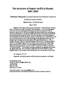
The trade reforms, with an aim of promoting exports and more efficient allocation of resources led to the initiation of SAPs in early 1980s. Kenya became the first recipient of these funds in sub-Saharan Africa (SSA) in the 1980s. The reforms included a shift from quantitative restriction to tariff equivalent, public sector reforms, and privatizations among others. The implementation of these reforms was ineffective due to various challenges such as poor macroeconomic performance, poor governance, and poor consultation and coordination between the government, donors and private sector (Odhiambo and Otieno, 2005). In 1986, the government renewed efforts towards reforms that led to the development of Sessional Paper No.1 of 1986, which advocated for export promotion and marked a clear departure from import substitution to export promoting policies. The benefits of the renewed policies could not be achieved due to market restrictions. The need for further comprehensive trade liberalization reforms in early 1990s was due to high tariff rate, overvalued exchange rate, the dismal performance of the export schemes, and incentive co-existing with poor macroeconomic performance and fiscal indiscipline (Were, Sichei and Milner, 2009). In 1993, major policies were implemented: floating of exchange rate, current and capital account restrictions were removed, elimination of trade licensing requirement, and restructuring of tariffs among others (Mwega and Muga, 1999). Despite these interventions, the increase in imports has always surpassed exports (Figure 2.1). Overtime, GDP, exports and imports have increased significantly but at a different pace, leading to a widening gap between them. In 1960, the level/size of GDP, exports and imports were relatively the same with a difference of only US$ 0.5 billion. However, by 1975, the gap between them had already emerged since Figure 2.1: Trend of GDP, imports and exports

Source: World Bank, 2012

6

Trade and economic performance

exports and imports remained more or less at the same level, while GDP increased. Within this period, import substitution approach was in operation. At the point of implementation of SAPs, which led to liberalization of goods and capital markets in 1993, the gap between GDP and imports had increased to US$ 3.5 billion, while that of exports and imports was at US$ 0.2 billion. In 1993, GDP experienced a significant drop. The effect was slight for imports, while exports remained stable due to the opening up of the markets and floating of exchange rate which led to stiff competition. In the period following liberalization, significant increase in all the three series was experienced, with GDP increasing faster while exports increased least leading to emergence of significant imports–exports gap, and which have increased ever since then to stand at US$ 5.6 billion by 2011. From 2003, a significant increase in GDP, exports and imports can be attributed to the change in political regime, which boosted the level of confidence in the country, and was a period of increasing economic growth. This indicates that trade can be determined by both economic and non-economic factors. The burgeoning import level and the widening gap seem to have started at around 1993, and the trend has been increasing ever since. Furthermore, while increase in exports has been insufficient to cover for imports, current account deficit has been persistent and widening. The penetration rate (the ratio of exports/imports to GDP) shows major fluctuations on this rate coincide with periods experiencing external and/or internal shocks. The oil crisis (1974), coffee boom (1978) and the liberalization period (1993) have had significant impact on Kenya trade. Both imports and exports’ penetration rate had a declining tendency in the 1960s, but the external shocks of oil and coffee prices affected GDP adversely leading to temporary increased imports and exports penetration rate. In 1980s, the poor economic and trade performance led to further decline in penetration rates, to a low of 21 per cent for exports and 26 per cent of imports. The economic and trade liberalization led to a loss of US$ 2.4 billion of GDP in 1993, hence the penetration rate of imports and exports had a positive inclination, with the slope of import being steeper and at a higher rate (World Bank, 2012). Import penetration rate recorded the highest rate of 46 per cent in 2011, while exports penetration rate stood at 29 per cent, which is the highest in more than a decade. The gap between exports and imports has been deteriorating overtime from approximately US$ 12 million in 1961, to US$ 33 million deficit by 1992. By 2011, the trade deficit stood at US$ 5.6 billion (approximately 10% of GDP), which is the highest to be ever recorded since independence (Figure 2.3). To understand and keep in check the worsening trend of trade deficit that seems to be driven

7

Import structure and economic growth in Kenya

Figure 2.2: Imports and exports penetration rate

Source: World Bank, 2012 by growing imports, there is need to understand the drivers and determinants of imports in Kenya. On the composition, approximately 30 per cent of Kenya imports consist of machinery and transport equipment, which can be interpreted in the light of the government’s aim of boosting productive potential. Kenya, like most developing countries, faces the challenge of low capital stock in their endeavour to achieve economic development. The major objective is to build up productive capacity through imports as well as to enhance productive efficiency within the country to spur economic growth and development in future. Mazumdar (2001) noted the import of capital goods stimulates growth based on the argument they boost the productive capacity of the economy. Moreover, they bring with them embedded technology, which if broken down and incorporated in the local production process, imported goods can be manufactured locally, hence reducing import bill in future. Also notable is the substantial imports of industrial supplies which could probably be used as intermediate goods together with the machinery and capital goods in the production process, hence increased productivity. Nevertheless, this has not been the case in Kenya since the current account deficit problem and import dependence has been growing over the last two decades. Kenya’s imports can be broadly classified into five categories (Figure 2.4). In the last ten years (2001-2011), on average, 23 per cent of imports comprise fuels and lubricants, 30 per cent constitute machinery and transport equipment, while industrial supplies which could be considered as intermediate goods consist of 31 per cent. Approximately 16 per cent of imports constitute food and consumer goods.

8

Trade and economic performance

Figure 2.3: Trend of trade balance

Source: World Bank, 2012 The lack of productive capacity locally justifies significant share of productivity enhancing imports to enhance the country’s capacity to produce more output (see the trend of each category in Figure 2.4). Imports of capital goods can stimulate the economy through growth and innovation channels, hence Kenya imports of industrial supplies and capital goods to a tune of 57 per cent in 2011 should enhance growth, which further motivates more imports and increased output. Focusing on the source of imports, the Middle East and Asian countries mostly United Arab Emirates, India and China, are the leading exporters to Kenya. In 2011, these countries contributed about 37.4 per cent of total imports to Kenya with United Arabs Emirates taking a share of about 15.2 per cent. These countries Figure 2.4: Imports by broad economic category

Source: Kenya National Bureau of Statistics, Various

9

Import structure and economic growth in Kenya

Figure 2.5: Source of Kenya imports 2.5a. Share of imports by region of origin

Source: Kenya National Bureau of Statistics, Various 2.5b. Share of imports by country of origin

Source: Kenya National Bureau of Statistics, Various share has been increasing remarkably from 21.1 per cent in 2001 to 37.4 per cent in 2011. Kenya’s crude oil is imported from the United Arab Emirates, while imports of capital and consumer goods are mainly imported from India and China. Imports from Europe and USA have been declining steadily from 33.8 per cent and 9.2 per cent in 1999 to approximately 19.4 per cent and 6 per cent in 2011, respectively. On the other hand, imports from Africa have been relatively stable averaging approximately 12 per cent, mainly from South Africa. The shift in the source of imports reflects a significant tendency towards trade with the East and a shift from America and Europe.

10

3.

Review of Literature

3.1

Theoretical Literature

Competitiveness and foreign and domestic economic activities were traditionally viewed as the main determinants of imports and exports (Camarero and Tamarit, 2003). However, theories of international trade have been evolving over time. Some of the earlier theories include; absolute advantage theory developed by Smith (1776) and Salvatore (1990), and comparative advantage theory developed by Ricardo (1817). Ricardo argued each country should specialize in the goods or services it can produce with the lowest cost, that is the goods and services it has a comparative advantage. Haberler (1936) further developed the opportunity cost theory arguing a nation has a comparative advantage if the cost of producing a certain commodity is lower than the cost of producing other commodities in that country relative to other countries, owing to differences in endowments. Most of the developing countries, Kenya included, are labour abundant, relative to capital and skilled labour. This implies that these countries will benefit if they produce goods that require relatively large amounts of unskilled labour, and exchange with capital and skilled labour intensive goods produced by the developed countries. In this case, they have a comparative advantage in producing labour-intensive goods and services. Heckscher, Ohlin and Samuelson (Jeffrey, 1990) have extended these theories to show how factor proportions can determine comparative advantage such that countries with a lot of labour relative to capital, for example, will tend to have a comparative advantage in the production of labour intensive goods and import the capital intensive goods that use scarce resources to produce. The theoretical relationship between imports, economic growth and productivity tends to be more complicated than between exports and economic growth (Ugur, 2008). Increased import of consumer products encourages domestic import-substituting firms to innovate and restructure them in order to compete with foreign competitors, thus augments efficiency in production. With increased competition and productivity, there is expansion in investments in new technology. Further, imports of capital goods boost productive capacity hence increasing efficiency and output. Productivity growth triggers economic growth and increases income, which in turn stimulates more imports. On the other hand, increased productivity in an import-substituting industry may crowd out imports. According to Grossman and Helpman (1991), imports of capital and intermediate commodities that cannot be produced domestically facilitate domestic firms to diversify and specialize, while sophisticated technology imports are helpful for efficient production and industrial development.

11

Import structure and economic growth in Kenya

The importation of capital goods for the manufacturing sector can be seen from two perspectives. On one hand, growth-oriented argument focuses on the role of capital goods in realizing new manufactured goods, which stimulate other sectors, increasing the level of output, hence economic growth. On the other hand, innovation-oriented approach considers the importance of capital goods as sources of new technology to the manufacturing sector. Diffusion of embodied technology to domestic industry from developed countries is important to increase productivity growth throughout the economy and this raises domestic output, hence economic growth. This is because exposure to new products generates knowledge and innovation that further reduces the cost of current production and future scientific innovations (Humpage, 2000). Different transmission mechanisms have been discussed in literature on the nexus between imports and economic growth. On one hand, through imports there is enhanced productivity, hence improved economic growth (Grossman and Helpman, 1991; Barro and Sala-i-Martin, 1992). This is because imported machinery is more efficient compared to the domestic ones (Coe, Helpman and Hoffmaister, 1997; Mazumdar, 2001). Moreover, imported goods have high technology and innovation embedded in them, and through learning, this technology can be transferred from developed to developing economies. On the other hand, the diffusion mechanism from the import perspective is based on the argument that higher demand for imports is experienced when income in a country increases, leading to more purchasing power, hence increased demand of domestic and foreign goods. 3.2

Empirical Literature

There are mainly five types of models with regard to aggregate estimating import demand function. The traditional model with income measured as real GDP, the revised traditional model with income measured as the real value of GDP minus exports, the disaggregated GDP model, the dynamic structural import demand model, and the structural model that incorporates a binding foreign exchange constraint (Senhadji, 1998; Emran and Shilp, 2010; and Zhou and Dube, 2011). Noteworthy is the fact that different uses of income and the components of imports have varying relationships where income is categorized by demand composition and imports by Standard International Trade Classification (SITC). To this end, some studies have adopted the disaggregated data on imports and incomes. Narayan and Narayan (2005) and Bathalomew (2012) have decomposed GDP into consumption, and investment and exports expenditure. The aim of this exercise is to underscore the various uses the incomes are committed to and

12

Review of literature

the implication of this on imports. Bathalomew (2012) finds consumption and government expenditure to have a significant effect on imports in Sierra Leone; while Frimpong and Oteng-Abayie (2006) conclude investment and exports components of income are the major determinants of import trend in the long run, and household and government expenditure are significant in the short run in the case of Ghana. On the other hand, some studies have focused on imports in a specific sector. Ghosh (2004) used disaggregated data focusing on import of crude oil in India, applying autoregressive distributed lag (ARDL) bound testing approach to cointegration. He concludes that a long run equilibrium relationship exists among quantity of crude oil imported, income and price of the imported crude, and there exists a unidirectional long run causality running from economic growth to crude oil import. Hye (2011) focusing on agricultural sector, confirmed long run association exists between agricultural growth and agricultural raw material imports, and also found a bidirectional causality. Baiyegunhi and Sikhosana (2012) focusing on wheat imports in South Africa concludes that income is a significant determinant of wheat imports. For the import and economic growth link to be strong, there is need for complimentary and consistent macroeconomic and structural policies that foster adjustment. Aldan, Bozok and Gunay (2012) found that income is more important compared to exchange rate in determining imports in most of the sectors. Similarly, Aydin, Çıplak and Yücel (2004) found higher income elasticities both in short run and long run. In India, Mishra (2012) argues for long run relationship between import and economic growth. In Ethiopia, the level of income has been documented as a positive and significant determinant of imports (Solomon, 2000). Various approaches have been adopted to underscore the nature of relationship between imports and economic growth. Ghosh (2004); Zhou and Dube (2011); Rashid and Razzaq (2010); Narayan and Narayan (2005); and Fida, Khan and Sohail (2011) used autoregressive distributed lag (ARDL) bounds testing approach of co-integration, while Mishra (2012) applied vector error correction estimates and Granger causality tests. Egwaikhide (1999), Kalyoncu (2006) and Osei (2012) adopted the Johansen Co-integration. Kotan and Saygili (1999); Aydin, Çıplak and Yücel (2004); and Ugur (2008) used Vector Autoregressive model, which is based on the assumption that all variables are endogenously determined, while Aldan, Borok and Gunay (2012) applied Kalman Filter approach. In this study, we adopt co-integration and error correction model for the analysis. Co-integration and error correction mechanisms are used to separate the long run and short run relationship between imports and GDP and their sub-categories.

13

Import structure and economic growth in Kenya

Limited studies on the relationship between imports and economic growth for developing countries, especially SSA exist. In Ghana, Osei (2012) argues import trade is crucial to economic growth, especially intermediate and capital goods imports. Bathalomew (2012) in Sierra Leone concludes consumption and government expenditure have the highest impact on imports in the short run, while relative prices are insignificant both in the long run and short run. N’Guessan bi Zambe, Yoaxing and Yue (2010) empirically examined the import demand function in the case of Cote D’Ivoire and found that investment and exports are the main determinants of imports in the long run. In Kenya, Mwega (1993) applying error correction models found that price and real income are insignificant, while foreign exchange reserves and earnings were significant in determining import level. Krishna, Ozyildirim and Swanson (2003) argues the direction of causality differ between developed and developing economies, while Islam, Hye and Shahbaz (2011) find long run bidirectional causality for high income countries but not for developing ones. The empirical literature gives mixed results on the import-GDP nexus, which creates a need for case specific studies. With the significant proportion of imports in international trade and the mixed results in the literature, there is need for up to date and country specific studies that illuminate on the dynamics of imports and economic growth. The present study explores the relationship between imports in Kenya and economic growth by using data for the period 1975-2011.

14

4.

Methodology

4.1

Theoretical Framework

The import demand model is based on the microeconomic consumer theory where the quantity of imports demanded is determined by the domestic and foreign price and income that exist in the economy. Following Mayes (1981); and Hye and Mashkoor (2010), we have an import demand function of the form: M = f (Y , Pm , Pd ) However, due to endogeneity in the prices, a relative price is used: M = f (Y , Pm / Pd ) Therefore, the import demand function can be represented as:

M = τ Y β1 p β2

(1)

where M is the imports, Y is income measured by GDP and is relative price between foreign (Pm) and domestic (Pd) prices, and τ is a constant term. By logarithmic transformation, which reduces heteroscedasticity, we get:

ln M t = τ + β1 ln Yt + β 2 ln Pt + υt

(2)

where Vt is the random term that captures the effect of variables that cannot be explicitly captured in the equation, they are time variant and it is expected that β1 > 0 and β 2 < 0 . Further, other explanatory variables are incorporated to augment the model such as foreign reserves, FDI and a measure of trade openness. For a developing economy, the level of reserves is very important for economic and financial stability, while the nature and level of FDI attracts imports of capital resources that are not available locally. 4.2

Empirical Model

The model as described in equation 2 is augmented by incorporating other macroeconomic explanatory variables. In line with the existing literature namely Dash (2005) and Osei (2012), an import demand model is adopted as stated in Equation 3:

lnRim t = β o + β1lnRGDPt + β 2ln Re rt + β 3 ln FDI + β 4 Inlf t + β 5ln Re srvt + β 6 ln trade + ε t

(3)

where: InRim is the log of real imports of goods and services;

InRGDP is the log of the domestic economic activity variable proxied by the real gross domestic product;

15

Import structure and economic growth in Kenya

LnFDI is the log foreign direct investment net inflows; LnRer is the log of real exchange rate adjusted for relative prices; Infl is the inflation rate; lnResrv is the log of foreign reserves; lntrade is the log of trade openness measured by the ratio of trade to GDP; e is the error term; and β i ‘s are elasticities.

Consistent with demand theory, imports are negatively related to relative prices and positively related to income, hence β1 > 0 and β 2 < 0 . We assume an imperfect substitute model where neither exports nor imports are perfect substitutes for domestic goods. Further, we assume world supply of imports to Kenya is perfectly elastic, since Kenya imports are a negligible share of world imports (Sinha, 1997). A dynamic model with a lag of imports as an independent variable is estimated. In addition, a lag structure is included such that an overparameterized equation is estimated following Hendry, Pagan and Sanyan (1986) and Egwaikhide (1999). Depending on the significance level, elimination of highly insignificant variables is implemented until we have an optimal model.

LnRimt = α o + α1 ( L)ln Rimt −1 + α 2 ( L) LnRGDPt + α3 ( L)ln RFDIt + α 4 ( L) Ln Re rt + α5 (L)Inlft + α 6 (L)Ln Re srvt + α 7 (L)ln trade +ν t

(4)

In addition, the national income as measured by GDP is decomposed to its constituent components of consumption and investment similar to Ho (2004), Narayan and Narayan (2005), and Magnus and Oteng-Abaiye (2006), with an aim of analyzing component expenditure effect on imports. Oil imports contribute about a quarter of total Kenya imports, hence the study considers an overall import model and another one that excludes oil imports. The main idea here is to assess if the elasticity differs significantly for the two models, and whether the exogenous shock of oil would affect the magnitude and significance of elasticities of the variables of interest. Co-integration approach is adopted in this study. When the variables are cointegrated, that is, they have long run equilibrium, Engel and Granger suggested an Error Correction Model (ECM) is applied to assess a short run relationship. To capture the short run effects and speed of adjustment, we estimate the following error correction model: k −1

k −1

k −1

k −1

k −1

k −1

k −1

i −1

i =0

i =1

i =0

i =0

i =0

i =0

� LnRimt = α0 + ∑α1� LnM t−i + ∑α2 � LnRGDPt−i + ∑α3� LnFDIt−i + ∑α4 � Ln Re rt−i + ∑α5 �inf lt−i + ∑α6 � LnRresrt−i + ∑α7 � Lntradet−i + α8 ECTt−1 + ε t

16

(5)

Methodology

The short run part is captured by the coefficients of the differenced variables, while the speed of adjustment in each period is given by the coefficients on error correction term (ECT). This parametre shows the amount of disequilibrium corrected in each period. The magnitude of these elasticities will influence the effectiveness of import trade policies. 4.3

Granger Causality

In estimating the causal relationship between imports and economic growth, the Granger causality test is used. Granger (1969) developed a test to check whether or not the inclusion of past values of a variable X improves the prediction of present values of variable Y. If the prediction of Y is improved by including past values of X relative to only using the past values of Y, then X is said to Granger-cause Y. In the same argument, if the past values of Y improve the prediction of X relative to using only the past values of X, then Y is said to Granger-cause X. If both X is found to Granger-cause Y and Y is found to Granger-cause X, then a feedback relationship exists. To implement the Granger test, a particular autoregressive lag length p is assumed and the following approach is applied: ∞ ∞ ln Rimt = ∑ α i ln Rimt −i + ∑ βi ln rgdpt −i + ε t i =1 i =1 ∞ ∞ ln rgdpt = ∑ηi ln rgdpt −i + ∑ λi ln Rimt −i + υt i =1

(6)

i =1

Therefore, there is Granger causality when the coefficient of one variable is not equivalent to zero in one equation, while the coefficient of the other variable is zero in the complementary equation. For instance, there is Granger causality from economic growth to imports if βi ≠ o and λ = 0 for all i. 4.4

Order of Integration

To stem the problem of spurious regression, it is important the time series properties of the data set employed in estimations are ascertained. The first step in time series regression analysis is to test the order of integration of each variable. In this case, the order of integration is determined by the unit root test. In determining the unit root test, the Augmented Dickey-Fuller (ADF) test is employed based on the following regression model: k

∆ Yt = a0 + a1T + a2Yt −1 + ∑ d j ∆Yt − j + ε t j =1

(7)

where ε t is pure white noise error term, Yt is time series, ∆ is the first difference operator, T is the time trend, α 0 is a constant and k is the optimum number of lags. A decision is taken based on the following rule: if the t-statistic associated

17

Import structure and economic growth in Kenya

with estimated coefficient is less than the critical value in absolute terms, then we conclude the series is non-stationary. 4.5

Co-integration Test

Likewise, it is important to test whether a long run equilibrium exists among the non-stationary economic variables. In this case, co-integration analysis is used to ascertain if the variables are co-integrated. To test for co-integration, there are two main approaches: Engle and Granger (1987) two step procedure, and Johansen (1988) and Johansen and Juselius (1990) maximum likelihood approach. This study adopts the Engle and Granger (1987) two-step procedure, which involves in the first step, the estimation of the co-integrating regressions followed by a unit root test on the residual. If the residual is stationary, then the independent and dependent variables have long run relationships (Rao, 1994). The drawback of this procedure is that it is difficult to determine the number of equilibrium relationships where many variables exist. The study used annual secondary data obtained from UNCOMTRADE, World Bank database and KNBS for the period 1975-2011.

18

5.

Results and Discussion

5.1

Descriptive Statistics

Table 5.1 shows the descriptive statistics of the data. It describes data in terms of measures of tendency and dispersion. Table 5.1: Descriptive statistics RIM

RGDP

RGDP_ CON

RGDP_ INVT

TRADE

RESERVES

INFL

FDI

RER

Mean

3.49

11.20

9.92

2.04

60

1.05

13

0.07

19.18

Median

2.48

10.70

8.77

1.58

58

0.52

11

0.03

13.99

Maximum

9.69

19.90

18.30

5.27

75

4.32

46

0.69

81.07

Minimum

1.11

5.22

4.55

1.02

48

0.05

2

-0.00

0.37

Std. Dev.

2.32

3.99

3.91

1.08

7

1.20

9

0.12

21.72

Skewness

1.10

0.44

0.45

1.54

0.26

0.66

1.03

1.99

1.39

Kurtosis

3.19

2.37

2.14

4.05

2.10

3.54

3.64

4.41

3.41

Source: Authors’ computation Note: Imports, GDP, consumption expenditure, investment expenditure, reserves and FDI are in billions

The kurtosis and skewness values should be about three and zero respectively, to indicate that the data is normally distributed and has bell-shaped distribution. The result indicates, apart from FDI and inflation, the other variables meet the criteria of normal distribution. Using the Akaike (AIC) and Schwarz Information Criterion (SIC), the optimal lag length of two is determined for the data. Table 5.2 presents the correlation results which attempt to establish the nature of association between variables. Besides, it is also a preliminary indicator on the existence or otherwise of multicollinearity. When the correlation is above 0.5, it Table 5.2: Correlation matrix RIM1 RIM1

RGDP

RGDPCON

RGDPINVT

TRADE

RESERVES

INFL

FDI

RER

1.00

RGDP

0.74

1.00

RGDP_CON

0.75

0.99

1.00

RGDP_INVT

0.97

0.88

0.88

1.00

TRADE

0.38

0.20

0.19

0.39

1.00

RESERVES

0.45

0.77

0.87

0.87

0.40

1.00

INFL

-0.15

-0.12

-0.18

-0.16

0.37

-0.17

1.00

FDI

0.52

0.46

0.46

0.54

0.31

0.58

-0.02

1.00

RER

0.85

0.95

0.96

0.74

0.33

0.73

-0.16

0.44

Source: Authors’ computation 19

1.00

Import structure and economic growth in Kenya

indicates the presence of multicollinearity. There exists a negative correlation between real imports and inflation and a positive relationship with all the other variables. Notable are the more than 0.50 per cent coefficients for real GDP and its components, real exchange rate, and foreign reserves which could be an indicator of multicollinearity. There are many approaches to addressing this problem, one of them is to drop the variable suspected to cause multicollinearity while assessing for a significant change in R-squared and the F-statistics. Following this process, we identified there is no significant challenge of multicollinearity in the analysis. Further, this is an indicator of endogeneity, but when statistical tests are carried out, the results are not significant since there is only one cointegrating vector that is significant. 5.2

Unit Root Tests

The Augmented Dickey Fuller (ADF) test was applied to test for stationarity. The main aim was to evaluate if the mean and variance of the variables have been constant overtime. When the test was applied at level data, the results indicated the variables are non-stationary with intercept and trend as shown in Appendix Table A1. We, therefore, accept the null hypothesis of unit root given that the test statistic is smaller than the coefficients in absolute terms apart from inflation. When the variables are differenced, we fail to accept the null of unit root since the test statistic is larger than the coefficients in absolute terms, which reflects the variables are stationary, hence integrated of order one as shown in Table 5.3. Table 5.3 shows the test statistic values on first difference are all significant at 1 per cent apart from real GDP which is significant at 5 per cent, indicating the variables are stationary. Since all variables are integrated of the same order, the next step is to test for direction of co-integration and causality. Table 5.3: Unit root tests Test statistic

1%

5%

10%

p-value

Order

Imports

-3.661

-3.682

-2.972

-2.618

0.0047

I(1)

GDP

-3.054

-3.682

-2.972

-2.618

0.0302

I(1)

FDI

-9.433

-3.682

-2.972

-2.618

0.0000

I(1)

Exchange rate

-5.063

-3.682

-2.972

-2.618

0.0000

I(1)

Reserves

-6.238

-3.682

-2.972

-2.618

0.0000

I(1)

Openness

-6.341

-3.682

-2.972

-2.618

0.0000

I(1)

Rgdp_Consumption

-6.223

-3.682

-2.972

-2.618

0.0000

I(1)

Rgdp_Investment

-6.014

-3.682

-2.972

-2.618

0.0000

I(1)

Source: Authors’ computation

20

Results and discussion

5.3

Co-integration Tests

Having obtained the result on stationarity, the next step is to test for co-integration, which aims to establish if a long run relationship exists between the variables. The appeal of co-integration is that it provides a formal framework for testing long run models from actual time-series data. The co-integration technique allows application of non-stationary data, while avoiding spurious regression results. The Engel-Granger co-integration test stipulates the variables have to be integrated in the same order, and there should exist a linear combination of the two variables. Granger (1983) showed that if two variables are co-integrated, then they have an error correction representation such that a significant and negative coefficient of the error correction term indicates a stable long run equilibrium between the variables. To test for co-integration, the primary model is estimated as described in equation 3. In this case, the main variables of interest are the real GDP, which present the level of income in the country and the real exchange rate adjusted for relative prices, which reflects the prices. Considering theoretical foundations, reserves, trade openness and FDI are further included arguing that more FDI attracts more imports, while adequate foreign reserves can contain more imports without effects on exchange rate. The results are presented in Table 5.4 in which part 1A presents results using overall imports as a dependent variable, while part 2A indicates results of imports excluding oil as a dependent variable. Further in each part there are four models, models 1 and 2 apply aggregate GDP, while models 3 and 4 use disaggregated GDP comprising consumption and investment demand. Models 2 and 4 are dynamic which incorporate a lag of the dependent variable. GDP is then disaggregated into consumption and investment expenditure. The disaggregate model not only avoids the problem of aggregation bias, but helps in estimating the separate effects of each GDP component on import demand. Since all variables are in natural logs apart from inflation, they are interpreted as elasticities. Real GDP reports the highest import elasticities both for overall imports and non-oil imports model ranging from 1.27 to 1.69, which reflects 1 per cent increase in incomes leading to 1.27 to 1.69 per cent increase in imports. The income elasticities for non-oil imports are lower compared to those of the overall imports model in all models, such that the elasticity declines to 1.65 from 1.69. In the case of dynamic model, the elasticity declines from 1.40 for overall imports model to 1.27 for non-oil imports. This means higher economic growth rate in Kenya will lead to more than proportionate increase in total imports, which is in line with the theory.

21

Import structure and economic growth in Kenya

Table 5.4: Regression results Table 1A-Total imports Model 1 GDP

Model 2

Table 2A-Non-oil imports

Model 3

Model 4

1.40***

1.65***

1.27***

[0.186]

[0.230]

[0.220]

[0.281]

1.53*** [0.186]

GDP_ Investment

0.39*** [0.092]

[0.078]

Reserves

Openness

FDI

Inflation

Adjusted R2 DW P(F-stat)

Model 3

1.34***

Model 4

1.69***

1.61***

[0.161]

[0.189]

[0.207]

0.31***

0.35***

0.31***

[0.094]

[0.098]

-0.66***

-0.51***

-0.68***

-0.56***

-0.62***

-0.45***

-0.67***

-0.62***

[0.036]

[0.070]

[0.034]

[0.041]

[0.043]

[0.082]

[0.034]

[0.054]

0.13***

0.11***

0.010

0.017

0.08*

0.07*

-0.034

-0.025

[0.038]

[0.033]

[0.031]

[0.025]

[0.045]

[0.039]

[0.031]

[0.032]

1.46***

1.22***

1.26***

1.13***

1.51***

1.26***

1.32***

1.28***

[0.210]

[0.196]

[0.125]

[0.107]

[0.248]

[0.232]

[0.128]

[0.131]

0.001

-0.005

-0.006

-0.010

0.000

-0.015

-0.007

-0.011

[0.018]

[0.016]

[0.011]

[0.009]

[0.022]

[0.020]

[0.011]

[0.011]

-0.002

-0.003

0.002

0.000

-0.005

-0.007

-0.001

-0.002

[0.003]

[0.003]

[0.002]

[0.001]

[0.003]

[0.003]

[0.002]

[0.002]

Imports lag

Constant

Model 2

1.69***

GDP_ consumption

Exchange rate

Model 1

0.25**

0.20***

0.30**

0.080

[0.098]

[0.052]

[0.119]

[0.072]

-28.3***

-24.9***

-29.4***

-26.5***

-26.9***

-22.3***

-31.7***

-30.5***

[4.276]

[4.434]

[3.270]

[2.780]

[5.034]

[5.357]

[3.335]

[3.579]

0.96

0.97

0.99

0.990

0.94

0.95

0.99

0.99

1.31

1.90

1.34

1.81

0.86

1.26

0.89

1.81

0.00

0.00

0.00

0.00

0.00

0.00

0.00

0.00

***,** & * indicates 1%, 5% and 10 % significance level respectively -Parenthesis [ ] indicates the S.E Source: Authors’ computation With disaggregated GDP, consumption expenditure is the most influential ranging from 1.34 to 1.69 per cent. Contrary to aggregate GDP, consumption elasticities are higher for non-oil imports compared to overall imports model increasing from 1.53 for overall imports to 1.69 for non-oil imports. For the dynamic model, the coefficient for non-oil imports is 1.61 compared to the overall import model of 1.34. Inclusion of the lagged imports in the model has the effect of lowering the consumption demand elasticity marginally for both overall imports and non-oil imports. The higher import elasticities for consumption expenditure for non-oil imports compared to the overall imports model may infer that nonoil imports are more sensitive to consumption expenditure. The combination of

22

Results and discussion

a relatively large share in total demand (above 90% of GDP) and relatively large import elasticity conjectures that the marginal import content of consumption is very high compared to that of investment. For investment expenditure, 1 per cent increase leads to 0.39 per cent increase in overall imports, but 0.35 per cent increase in non-oil imports. These elasticities are lower when we consider the dynamic model, which posits the same magnitude of 0.31 per cent for overall imports and non-oil imports. Therefore, we could infer that investments are critical in determining non-oil imports. In the overall, import demand changes more than proportionately to changes in real GDP. This is expected since about 61 per cent of Kenya imports comprise intermediate and capital goods. As the economy grows, more of such goods are required to expedite the growing needs of the economy. The aggregate imports are fairly price inelastic with elasticity ranging from 0.45 to 0.68. Consequently, a 1 per cent depreciation of the real exchange rate leads to 0.45 to 0.68 per cent decline in imports. This could be explained by the fact that exchange rate depreciation would deteriorate demand for imports as foreign goods would be relatively more expensive. Furthermore, the elasticities for the non-oil imports model are generally lower compared to overall imports model, which suggests high sensitivity of oil imports to prices. Though the theory and empirical evidence stipulates the import elasticities of income and price should be unitary, that is, there is one-to-one relationship, this does not seem to hold for Kenya where the income elasticity is greater than one, while that of price is less than one. The overall and non-oil imports are elastic with respect to trade openness, where the elasticity ranges from 1.13 to 1.46, indicating that a 1 per cent increase in trade openness brings about more than proportionate increase in imports. Further, the coefficients for non-oil imports are higher which shows the higher sensitivity of non-oil imports to trade openness compared to overall imports. The imports have a positive and significant relation with the foreign exchange reserves for the model with aggregate GDP as expected, while the significance and magnitude of the coefficients decline for the non-oil imports. The FDI net inflows and inflation have negative coefficient and they are statistically insignificant. The lag of import is statistically significant with a magnitude between 0.30 and 0.20, implying that a 1 per cent increase in imports in the previous period leads to about 0.20 to 0.30 per cent increase in current imports.Though the coefficient is higher for the non-oil imports at 0.30 for the model with aggregate GDP, when the components of GDP are considered, the significance of the lag disappears. Overall, all the models have a reasonable goodness of fit as shown by adjusted R squared and DW statistic which are within acceptable regions, especially for the dynamic

23

Import structure and economic growth in Kenya

Table 5.5: Unit root test of the co-integrating vector Model

Test statistic

1%

5%

10%

p-value

Order

Residual 1A1

-4.7606

-3.682

-2.972

-2.618

0.0005

I(0)

Residual 1A3

-4.3159

-3.682

-2.972

-2.618

0.0016

I(0)

Residual 2A1

-3.5254

-3.682

-2.972

-2.618

0.0129

I(0)

Residual 2A3

-3.3149

-3.682

-2.972

-2.618

0.0215

I(0)

Source: Authors’ computation models. To determine if the variables are co-integrated, we test the unit root of residuals from the results above long run model. The variables are co-integrated if the error term is stationary at levels (that is,I(0)). The results are presented in Table 5.5. To determine if the variables are co-integrated, the ADF test for unit root was conducted on the residual. The results in Table 5.5 indicate the residuals are integrated of order zero, since they are stationary at levels. The co-integration test clearly establishes significant co-integration relationships on the basis of the ADF statistics, since we fail to accept the null hypothesis of non-stationarity. Since we are interested in both short run and long run import elasticities, we build an error correction model (ECM) which includes the long run co-integration (error correction term-ECT) vector and short run adjustments between the dependent variable and the explanatory variable. 5.4

Error Correction Models

With co-integration of variables confirmed, the next step is to estimate an ECM to obtain short run equilibrium and the speed of adjustment in case of a shock. Since the variables are integrated of order one, then we only include one difference in the error correction model. The error correction term shows the speed with which our model returns to equilibrium following an exogenous shock. It should have a negative sign, indicating a move back towards equilibrium; a positive sign indicates movement away from equilibrium. The coefficient should lie between 0 and 1, where 0 suggests no adjustment one time period later and 1 indicates full adjustment within one period. The ECM is formulated using the residual from the long run model lagged once as the error correction term (ECT). Therefore, if co-integration exists, the error correction term will be significant. The results are presented in Table 5.6. In the ECM, the coefficient of the changes of the independent variables indicate the short run effects. The changes in real exchange rate, trade openness, FDI net inflows and inflation have statistically significant short run effects on real imports.

24

Results and discussion

Table 5.6: Error correction model ECM

Table 1B - Total imports

Table 2B - Non-oil imports

Model 1

Model 1

Model 2

LDLNRIM

-0.020 [0.090]

DLNRGDP

1.25 [0.818]

DLNRGDPCON

0.87*** [0.238]

DLNRGDPINVT DLNRER

-0.067 [0.052]

Model 2 -0.025 [0.102]

-0.008 [0.049]

2.16* [0.948] 1.85*** [0.239] 0.39*** [0.066]

0.42*** [0.065]

-0.78*** [0.126]

-0.67*** [0.077]

-0.71*** [0.146]

-0.58*** [0.074]

DLNRESRV

0.0150 [0.036]

-0.021 [0.022]

0.007 [0.040]

-0.025 [0.021]

DLNTRADE

1.31*** [0.156]

1.12*** [0.102]

1.32*** [0.184]

1.08*** [0.099]

DLNFDI

-0.003 [0.008]

-0.004 [0.005]

-0.012 [0.010]

-0.013** [0.005]

DINFL

0.001 [0.002]

0.000 [0.001]

-0.003 [0.002]

-0.003** [0.001]

ECTLRES2

-0.42** [0.161]

-0.66*** [0.161]

-0.33** [0.141]

-0.52*** [0.155]

Constant

0.04 [0.045]

0.03 [0.019]

-0.001 [0.052]

-0.03 [0.019]

0.86

0.95

0.79

0.94

1.81

1.54

1.66

1.83

0.00

0.00

0.00

0.00

Adjusted R2 DW P(F-stat)

-***,** & * indicates 1%, 5% and 10 % significance level, respectively -Parenthesis [ ] indicates the S.E Source: Authors’ computation The specification of the ECM indicates that for overall imports, trade openness is the most influential factor with a sensitivity of between 1.32 and 1.12 for all models. Therefore, in the short run, changes in trade openness bring about more than proportional change in imports. However, these changes are lower in the short run compared to the long run elasticities of 1.46 and 1.51 for overall and non-oil imports model, respectively (Table 5.4). The real exchange rate has a negative sign and is statistically significant, while the magnitude of these changes are relatively higher in the short run (0.78) compared to the long run (0.66) for the overall model. Moreover, the changes are lower for the non-oil imports model (0.71)

25

Import structure and economic growth in Kenya

which imply oil imports might be highly sensitive to changes in real exchange rate compared to other imports. The ECM results illustrate that different GDP components have different effects on imports in Kenya. Noteworthy is the insignificance of aggregate GDP for the overall import model, while consumption expenditure change is less than unitary (0.87) implying the short run imports respond to change in consumption expenditure. Moreover, the investment expenditure is still significant and with the same magnitude, as in, the long run of such changes in investment expenditure leads to 0.39 changes in imports as shown in Tables 5.4 and 5.6. In addition, the coefficient for consumption and investment expenditure are rather high for nonoil imports model compared to the overall imports. For non-oil imports model, consumption expenditure reports a change of 1.85, which is even higher compared to the long run elasticity of 1.69 to 1.61 as in Table 5.5. A similar case also applies for investment whose coefficient is 0.42 compared to 0.35 to 0.31 in the long run. This implies that in the short run, non-oil imports are highly sensitive to consumption and investment expenditure compared to oil imports. In estimating the ECM, the speed of adjustment for the disequilibrium implied by the one period lagged ECT is strongly significant and has a negative sign in the range of 0.33 and 0.66. For the overall import with disaggregated GDP where 66 per cent of the adjustment is corrected every period, it means in 11/3 years, the disequilibrium will be wholly corrected. Generally, the speed of adjustment for overall imports is higher compared to the non-oil imports, with the lowest speed at 0.33, which suggests it will take approximately three years to correct the disequilibrium from the long run equilibrium. Therefore, any disequilibrium created in the short run will be temporary and will be corrected over time. The fact that the estimated adjustment coefficient is found to be negative in all cases confirms a significant co-integration relationship exists. Thus, for any disequilibrium in the short run level relationship, a corrective change in overall and non-oil imports is induced towards the long run equilibrium. The first estimation in the Engle-Granger two-step co-integration approach demonstrates in the long run that real GDP, consumption and investment demand, real exchange rate, trade openness, lagged real imports and partially foreign reserves significantly affect imports as shown in Table 5.4. Table 5.6 shows in the short run, consumption and investment expenditure, real exchange rate, trade openness and partially FDI net inflows and inflation have significant impacts on imports. However, the significance of GDP for overall imports model disappears in the short run, while for non-oil imports is only significant at 10 per cent though with a high sensitivity of 2.16. These results differ from those of Mwega (1993) who found income and prices were not significant determinants of imports. However,

26

Results and discussion

the results are high with most of the literature both in developing and developed countries as noted in the literature review, which finds the variables of income and price to be significant. The significance of foreign reserves is similar to the India study by Dash (2005) who finds them to be significant both in the short run and long run. As discussed in the methodology, an over parameterized model is also estimated to take care of any lags that might be significant drivers of imports. The results are presented in Apendix Table A2. The results indicate the over parameterized model with two lags. The number of lags was informed by the Akaike criterion.To obtain a parsimonious model, the over parameratized model was reduced by removing, sequentially, the lags of each variable with low t-values, and then using the F-test and Schwartz criterion to check the validity of the simplification. The starting point in the reduction process was to remove all lags with p-value greater than 0.70, followed by those greater than 0.50. Sequentially, specific lags that were found insignificant were then removed. The results confirm the real exchange rate and trade openness are significant determinants of imports, while the significance of real GDP disappears. Further, two periods lagged changes of inflation are now significant at 5 per cent though with a small magnitude. This implies 1 per cent increase in inflation in the past period increases current imports by 0.3 per cent. The stronger SIC and the significant F statistics confirm our model simplification is statistically valid. In the parsimonious model, the error correction term is significant at 10 per cent with a negative sign and a magnitude of 0.42. This confirms the variables are cointegrated and in case of a shock, 42 per cent disequilibrium is corrected in every period. The result of the post-estimation test shows that models are good in the sense that they satisfy the diagnostic test and have a high adjusted R squared. The error term is also found to be normally distributed. However, using the Chow Test for structural break, the result indicates there is a structural change in 1993, which coincides with the liberalization period. Therefore, a dummy is included in equation 4 and the following results are obtained as shown in Table 5.7. In line with the results discussed in Table 5.4, the signs of the coefficients have not changed with the inclusion of the dummy, but the magnitudes have changed slightly. The magnitude for the aggregate GDP have increased substantially with an average increase of 0.3 compared to results in Table 5.4, while overall imports elasticity for consumption and investment demand have remained relatively the same. For non-oil imports, elasticity for consumption demand has increased, while that for investment has slightly declined, which could be reflecting change in data generation process. The price elasticity of imports is relatively high ranging between 0.57 and 0.80. Though foreign reserves are still significant, the

27

Import structure and economic growth in Kenya

Table 5.7: Results including year dummy (1993) Table 1C - Total imports Model 1 GDP

Model 2

Model 3

Table 2C - Non-oil imports Model 4

Model 1

Model 2

Model 3

Model 4

1.37***

1.77***

1.67***

2.05***

1.72***

2.02***

1.59***

[0.226]

[0.259]

[0.273]

[0.345]

GDP_ consumption

1.55*** [0.207]

[0.175]

[0.208]

[0.224]

GDP_ Investment

0.39***

0.30***

0.33***

0.30***

[0.095]

[0.099]

Exchange rate

Reserves

Openness

FDI

Inflation

Dummy

[0.094]

[0.080]

-0.80***

-0.64***

-0.68***

-0.58***

-0.76***

-0.57***

-0.70***

-0.65***

[0.067]

[0.087]

[0.048]

[0.047]

[0.080]

[0.115]

[0.048]

[0.064]

0.01**

0.08**

0.009

0.02

0.05

0.05

-0.04

-0.03

[0.037]

[0.032]

[0.031]

0.026

[0.045]

[0.041]

[0.031]

[0.032]

1.35***

1.15***

1.25***

1.11***

1.39***

1.22***

1.31***

1.26***

[0.200]

[0.185]

[0.130]

[0.112]

[0.242]

[0.229]

[0.131]

[0.135]

0.009

0.002

-0.005

-0.010

0.008

-0.007

-0.006

-0.01

[0.017]

0.015

[0.011]

[0.009]

[0.021]

[0.020]

[0.011]

[0.011]

0.002

0.001

0.002

0.001

0.000

-0.003

0.000

-0.0007

[0.003]

0.003

[0.002]

[0.002]

[0.004]

[0.004]

[0.002]

[0.002]

-0.35**

-0.28**

-0.02

-0.03

-0.36**

-0.24

-0.08

-0.06

[0.143]

[0.124]

[0.079]

[0.067]

[0.172]

[0.161]

[0.079]

[0.081]

Imports lag

Constant

0.22**

0.20***

0.26**

[0.092]

[0.054]

[0.120]

0.08 [0.073]

-35.3***

-30.9***

-29.7***

-27.1***

-33.9***

-28.0***

-33.1***

-31.5***

[4.864]

[4.927]

[3.622]

[3.021]

[5.873]

[6.457]

[3.634]

[3.870]

Adjusted R2

0.97

0.98

0.99

0.99

0.95

0.96

0.99

0.99

DW

1.24

1.84

1.32

2.34

0.80

1.13

0.88

0.92

P(F-stat)

0.00

0.00

0.00

0.00

0.00

0.00

0.00

0.00

-***,** & * indicates 1%, 5% and 10 % significance level respectively -Parenthesis [ ] indicates the t-statistic Source: Authors’ computation magnitude has declined from about 0.13 to 0.01 for overall imports, but for nonoil imports the significance has disappeared. Trade openness generally declines across all models. Nevertheless, the dummy is only significant for the model with aggregate GDP. The goodness of fit for the model remains high as shown by adjusted R-squared.

28

Results and discussion

Table 5.8: Pair-wise Granger causality tests Null Hypothesis

F-Statistic

Prob.

LNRGDP does not Granger Cause LNRIM

7.96885

0.0017

LNRIM does not Granger Cause LNRGDP

1.35438

0.2734

Source: Authors’ computation 5.5

Causality Tests

Table 5.8 presents the results for Granger causality test. The results show a unidirectional causality from real GDP to real imports, that is, real GDP Granger causes real imports at 1 per cent significance level, but real imports do not Granger cause real GDP. Therefore, an increase in GDP can contribute to an increase in imports. For example, between 2003 and 2011, the Kenyan economy registered an average economic growth rate of approximately 4.6 per cent per annum, while imports increased from US$ 4.5 billion in 2003 to US$ 15.5 billion in 2011.

29

Import structure and economic growth in Kenya

6.

Conclusion and Policy Recommendations

Kenya is a small and open economy where international trade is important to its growth. Kenya’s imports have increased at a rapid rate in the last decade with economic growth averaging 4 per cent. This paper assessed the determinants of demand functions for imports in Kenya considering real GDP, foreign reserves, real exchange rate, FDI net inflows and trade openness. The central aim was to investigate the behaviour of Kenya’s aggregate and disaggregated import demand covering the period 1975 to 2011. The ECM approach was employed for analysis. The results show that in the long run, a relationship exists between real imports and real GDP, real exchange rate, trade openness and foreign reserves. The results reveal the ECT lagged once is negative and significant. This confirms a stable long run relationship exists among the real imports and its determinants. The statistical significance of the lagged error correction model suggests the aggregate import demand adjusts to correct shocks effect. In the short run, import demand is sensitive to real exchange rate, consumption and investment expenditure, FDI net inflows, inflation and trade openness. In analyzing the size of the coefficients with a disaggregated GDP (investment and consumption expenditure) model, the study finds prices, trade openness and domestic income as the most important factors determining the changes in imports in the long and short run. The empirical estimate shows that in the long run, imports are elastic with respect to income and inelastic with respect to price. The Granger causality test results, on the other hand, show a unidirectional causality from real GDP to real imports, that is, real GDP Granger causes real imports, but real imports do not Granger cause real GDP. Based on the empirical findings, the study suggests the following policy recommendations: First, GDP growth causes increases in imports. This implies economic growth is likely to worsen Kenya’s balance of payment difficulties. Considering consumption expenditure affects imports more than investment expenditure, imports should be restricted to intermediate and capital goods. Importation of raw materials for value addition and technology to expand capacity will improve productivity and output growth. Hence, policies, which discourage imports for direct consumption, should be put in place and this could be achieved by the use of selective import duty policies. The common external tariff under the customs union and imposition of excise tax will affect imports.

30

Conclusion and policy recommendations

Second, there is lower speed of adjustment for the non-oil imports with respect to consumption expenditure and trade openness. This implies monetary policies that work through the exchange rate and fiscal policies that work through government expenditure can be used as instruments to maintain favourable trade balance.

31

Import structure and economic growth in Kenya

References Aldan, A., Bozok, I. and Gunay, M. (2012), “Short Run Import Dynamics in Turkey,” Turkiye Cumhuriyet Merkez Bankasi, Working Paper No. 12/25. Aydın, F., Çıplak, U. and Yücel, M. E. (2004), “Export Supply and Import Demand Models for the Turkısh Economy,” Central Bank of the Republic of Turkey, Working Paper No. 04/09. Baiyegunhi, L. and Sikhosana, A. M. (2012), “An Estimation of Import Demand Function for Wheat in South Africa: 1971-2007,” African Journal of Agricultural Research, Vol. 7(3): 5,175-5,180. Barro, R. and Sala-i-Martin, X. (1995), Economic Growth, New York: McGrawHill. Bathalomew, D. (2012), “An Econometric Estimation of the Aggregate Import Demand Function for Sierra Leone,” Journal of Monetary Economic Integration, Vol. 10, No. 1. Bigsten, A. and Durevall, D. (2004), Trade Reform and Wage Inequality in Kenya: 1964-2000. Camarero, M. and Tamarit, C. (2003), “Estimating Exports and Imports Demand for Manufactured Goods: The Role of FDI,” European Economy Group Working Paper No. 22/2003. Coe, D. T., Helpman, E. and Hoffmaister, A. (1997), “North-South R&D Spillovers,” Economic Journal 107: 134-149. Dash, A. K. (2005), An Econometric Estimation of the Aggregate Import Demand Function for India, Aryan Hellas Limited, IBRC Athens. Egwaikhide, F. E. (1999), “Determinants of Imports in Nigeria: A Dynamic Specification,” African Economic Research Consortium Research Paper No. 91. Emran, M. S. and Shilp, F. (2010), “Estimating Import Demand Function in Developing Countries: A Structural Econometric Approach with Applications to India and Sri Lanka,” Review of International Economics, Vol. 18(2): 307-319. Engel, R. F. and Granger, W. J. (1987), “Co-integration and Error Correction Representation, Estimation and Testing,” Econometrica, Vol. 55(2), 251276.

32

References

Fida, B.A., Khan, M. M. and Sohail, M.K. (2011), “Revisiting Aggregate Import Demand Function in Pakistan using ARDL Methodology,” American Journal of Scientific Research, 33, 5-12. Frimpong, J. M. and Oteng-Abaiya, E. F. (2006), “Aggregate Import Demand and Expenditure Components in Ghana: An Econometric Analysis,” MPRA Paper No. 599. Ghosh, S. (2004), “Import Demand of Crude Oil and Economic Growth: Evidence from India,” Journal of Energy Policy, Vol. 37(2): 699-702. Granger, C. W. J. (1969), “Investigating Causal Relation by Econometric and Cross-Sectional Method,” Econometrica 37: 424–438. Granger, C. W. J. (1983), “Co-integrated Variables and Error Correcting Models,” UCSD Discussion Paper 83-13. Grossman, G. M. and Helpman, E. (1991), Innovation and Growth in the Global Economy, Cambridge: MIT Press. Haberler, G. (1936), The Theory of International Trade, London: William Hodge. Hendry, D. F., Pagan, A. R. and Sargan, J. D. (1986), “Dynamic Specification,” in Giliches, Z. and Intriligator M. D. (eds), Handbook of Econometrics, Vol. 3, Amsterdam, North-Holland. Ho, W. S. (2004), Estimating Macao’s Import Demand Functions, Monetary Authority of Macao. Humpage, O. F. (2000), Do Imports Hinder or Help Economic Growth? Economic Commentary, Federal Reserve Bank of Cleveland. Hye, Q. M. A. and Mashkoor, M. (2010), “Import Demand Function for Bangladesh: A Rolling Window Analysis,” African Journal of Business Management, Vol. 4(10): 2150-2156 Hye, Q. M. A. (2011), “Growth and Raw Material Imports Nexus: An Empirical Study of Pakistan’s Agricultural Sector,” Journal of Agricultural Research, Vol. 49(3): 407-418. Ismal, F., Hye, Q. M. A. and Shahbaz, M. (2011), “Imports-Economic Growth Nexus: ARDL Approach to Co-integration,” MPRA Paper No. 28462. Jeffrey, H. B. (1990), “The Heckscher-Ohlin-Samuelson Model: The Hinder Hypothesis and the Determinants of Bilateral Intra-Industry Trade,” Economic Journal, Vol. 100, 1216-1229.

33

Import structure and economic growth in Kenya

Johansen, S. and Juselius, K. (1990), “Maximum Likelihood Estimation and Inference on Co-integration with Applications to the Demand for Money,” Oxford Bulletin of Economics and Statistics 52: 169-210. Johansen, S. (1988), “Statistical Analysis of Co-integration Vectors,” Journal of Economic Dynamics and Control, 12(2–3), 231–254. Johansen, S. (1991), “Estimating and Testing Co-integration Vectors in Gaussian Vector Autoregressive Models,” Econometrica, 59, 1551–1580. Kalyoncu, H. (2006), “An Aggregate Import Demand Function for Turkey,” The Indian Journal of Economics, Vol. 86(4):503-511. Kotan, Z. and Saygili, M. (1999), “Estimating an Import Function for Turkey,” The Central Bank of the Republic of Turkey Discussion Paper, No. 9909. Krishna, K., Ozyildirim, A. and Swanson, N. R. (2003), “Trade, Investment and Growth Nexus, Analysis and Prognosis,” Journal of Development Economics, Vol. 70(2), 479–499. Magnus, J. F. and Oteng-Abaiye, F. E. (2006), “Aggregate Import Demand and Expenditure Components in Ghana: An Econometric Analysis,” Journal of Social Sciences, 4(1):1-6. Mayes, G.M. (1981), Applications of Econometrics, Prentice Hall, Inc. Mazumdar, J. (2001), “Imported Machinery and Growth in LDCs,” Journal of Development Economics, 65: 209-224. Mishra, P. K. (2012), “The Dynamics of the Relationship between Imports and Economic Growth in India,” South Asian Journal of Macroeconomics and Public Finance, Vol. 1(1): 57-79. Mwega, F. M. and Muga, K. L. (1999), Africa and the World Trade Systems: A Case Study of Kenya, AERC Report. Mwega, F. M. (1993), “Import Demand Elasticities and Stability during Trade Liberalization: A Case Study of Kenya,” Journal of African Economies, Vol. 2, 381-416. N’Guessan bi Zambe, S. C., Yoaxing, Y. and Yue Y. (2010), “An Econometric Estimation of Import Demand Function for Cote D’Ivoire,” International Journal of Business Management,Vol. 5(2): 77-84. Narayan, P. K. and Narayan, S. (2005), “An Empirical Analysis of Fiji’s Import Demand Function,” Journal of Economic Studies, Vol. 32(2), 158-168.

34

References

Ng’eno, N. K., Nyangito, H. O., Ikiara M., Ronge, E. and Nyamunga, J. (2003), “Regional Integration Study of East Africa: The Case of Kenya,” KIPPRA Working Paper No. 9. Odhiambo, W. and Otieno, G. (2005), Trade Policy Reforms and Poverty in Kenya: Processes and Outcomes. Osei, V. (2012), “Import Demand and Economic Growth Analysis in Ghana,” Journal of Economics and Sustainable Development, Vol. 3(14); 73-90. Rao, B. (ed.) (1994), Co-integration for the Applied Economist, New York: St Martin’s Press. Rashid, A. and Razzaq, T. (2010), “Estimating Import Demand Function in ARDL Framework: The Case of Pakistan,” MPRA Paper No. 23702. Reininger, T. (2008), “Factors Driving Import Demand in Selected Central, Eastern and Southeastern European Countries,” Focus on European Economic Integration, 1/08. Ricardo, D. (1817), “On the Principles of Political Economy and Taxation,” In P. Sraffa (ed.) (1951), The Works and Correspondence of David Ricardo,Vol. I, Cambridge: Cambridge University Press. Salvatore, D. (1990), International Economics Schaum’s Outline Series: Theory and Problems, 4th ed., New York: McGraw-Hill. Seim, L. T. (2009), FDI and Openness: Differences in Response across Countries. Senhadji, A. (1998), “A Time-Series Estimation of Structural Import Demand Equations: A Cross-Country Analysis,” IMF Staff Papers, Vol. 45(2). Sinha, D. (1997), “Determinants of Import Demand in Thailand,” International Economic Journal, Vol. 12:73–83 Smith, A. (1776), “An Inquiry into the Nature and Causes of the Wealth of Nations,” In R. H. Campbell, and A. S. Skinner (eds), The Glasgow Edition of the Works and Correspondence of Adam Smith, Vol. 2, Oxford: Oxford University Press. Solomon, K. (2000), The Structure and Behaviour of Import Demand in Ethiopia, Unpublished MSc. Thesis, Addis Ababa University, Ethiopia. Tang, T. C. (2003), “An Empirical Analysis of China’s Aggregate Import Demand Function,” China Economic Review, Vol. 12(2), 142-63. Ugur, A. (2008), “Import and Economic Growth in Turkey: Evidence from Multivariate VAR Analysis,” East-West Journal of Economics and Business, Vol. XI (1): 54-75. 35

Import structure and economic growth in Kenya

Were, M., Sichei, M. and Milner, C. (2009), Trade Policy in Kenya, Chapter 6. World Bank (2012), World Development Indicators, Washington DC: International Bank for Reconstruction and Development. Zhou, Y. and Dube, S. (2011), “Import Demand Functions: Evidence from CIBS,” Journal of Economic Development,Vol. 36 (4), 73-96.

36

Appendix Table A1: Unit root tests results at levels t- statistic

1%

5%

10%

p-value

Imports

2.732

-3.689

-2.975

-2.619

0.9991

GDP

0.769

-3.689

-2.975

-2.619

0.9911

FDI

-2.295

-3.689

-2.975

-2.619

0.1735

Inflation

-3.484

-3.689

-2.975

-2.619

0.0089

Exchange rate

-0.238

-3.689

-2.975

-2.619

0.9338

Reserves

3.725

-3.689

-2.975

-2.619

0.9999

Openness

-2.153

-3.689

-2.975

-2.619

0.2236

gdp_consumption

-0.199

-3.689

-2.975

-2.619

0.9297

gdp_investment

0.053

-3.689

-2.975

-2.619

0.9574

Source: Authors’ computation



37

Import structure and economic growth in Kenya

Table A2: Overparameterized error correction model Overparameterized

Parsimonious

DLNRIM(-1)

0.12

DLNRIM(-2)

0.17

0.20

DLNRGDP

0.55

0.97

DLNRGDP(-1)

0.37

DLNRGDP(-2)

0.05

DLNRER

-0.77*

DLNRER(-1)

0.25

DLNRER(-2)

0.14

0.29**

DLNRESRV

0.05

0.04

DLNRESRV(-1)

0.04

0.03

DLNRESRV(-2)

0.07

DLNTRADE

0.77***

0.75***

DLNTRADE(-1)

-0.08

0.10

DLNTRADE(-2)

-0.07

DLNFDI

0.00

DLNFDI(-1)

-0.01

DLNFDI(-2)

-0.01

DINFL

0.00

DINFL(-1)

0.00

-0.002

DINFL(-2)

0.00

-0.003**

RES2(-1)

-0.42

-0.29*

C

-0.03

-0.01

R2

0.92

0.91

DW

2.19

1.95

SIC

-1.24

-1.92

-0.76***

-***,** & * indicates 1%, 5% and 10% significance level, respectively Source: Authors’ computation

38