Confirming Pages
CHAPTER 9
Human Capital Theory: Applications to Education and Training LEARNING OBJECTIVES LO1 c Discuss how the decision to invest in human capital (schooling or on-the-job training) can be analyzed as a standard investment decision based on a comparison between the costs and benefits of the investment.
LO2 c Explain how the most expensive part of an investment in human capital is the opportunity cost of one’s time.
LO3 c Explain why trying to estimate the monetary return to education by simply comparing the earnings of more- and less-educated workers can be misleading due to the ability bias, or because education is used as a “signal” in the labour market.
LO4 c Describe how the return to education is quite large and has been increasing over time in Canada.
In the chapters on labour supply we emphasized the quantity aspects of labour supply, ranging from family formation to labour force participation to hours of work. Labour supply also has a quality dimension encompassing human capital elements such as education, training, labour market information, mobility, and health. In addition, in the previous chapter on compensating wages, we indicated that compensating wages may have to be paid to compensate workers for the costly process of acquiring human capital, like education or training. The approach developed in that chapter can be applied to costly attributes necessary to do a job, just as it can be applied to negative job attributes like risk. While the economics of education and health are often the subject matter of separate courses and texts, they—along with training, job search, and mobility—have a common theoretical thread: human capital theory. This chapter presents the basic elements of human capital theory and applies it mainly to the areas of education and training.
HUMAN CAPITAL THEORY LO1
The essence of human capital theory is that investments are made in human resources so as to improve their productivity and therefore their earnings. Costs are incurred in the expectation of future benefits; hence, the term “investment in human resources.” Like all investments, the key question becomes, is it economically worthwhile? The answer to this question depends on whether or not benefits exceed costs by a sufficient amount. Before dealing with the investment criteria whereby this is established, it is worthwhile to expand on the concepts of costs and
LO5 c Discuss the circumstances under which either workers or employers are the ones who should pay for training programs.
MAIN QUESTIONS •
Why are more-educated workers generally paid more than lesseducated workers? What factors determine the market rate of return to education?
•
If education is such a worthwhile investment, why doesn’t everyone have a Ph.D.?
•
Are more-educated people paid more because of the learning they acquired, or do higher education levels merely indicate these individuals’ inherently greater productivity?
•
What is labour market signalling and screening? How might education serve a role as a signal? If education is used primarily as a screening device, why might the private and social rates of return to education diverge?
•
Should the government subsidize early childhood learning programs?
•
Are government-funded training programs worth the money? 243
ben40208_ch09_243-279.indd 243
03/10/11 11:44 AM
Confirming Pages
244
www.epinet.org
PART 4: The Determination of Relative Wages
benefits as utilized in human capital theory. In this chapter, only the basics are touched upon. A wealth of refinements and precise methodological techniques is contained in the extensive literature on human capital theory and its application. In calculating the costs of human capital, it is important to recognize not only direct costs, such as books or tuition fees in acquiring university education, but also the opportunity cost or income foregone while people acquire the human capital. For students in university or workers in lengthy training programs, such costs can be the largest component of the total cost. The evaluation of these opportunity costs can prove difficult because it requires an estimation of what the people would have earned had they not engaged in human capital formation. In addition, it is important to try to distinguish between the consumption and the investment components of human capital formation, since it is only the investment benefits and costs that are relevant for the investment decision. In reality, this separation may be difficult or impossible—how does one separate the consumption from the investment benefits of acquiring a university degree? For example, a consumption benefit of studying English literature is that it helps one appreciate and enjoy reading old novels. Studying literature also helps improve one’s writing, which is an investment benefit that is highly valued in a modern economy. Nevertheless, the distinction between consumption and investment benefits must be made qualitatively, if not quantitatively, especially in comparing programs where the consumption and investment components may differ considerably. A distinction must also be made between private and social costs and benefits. Private costs and benefits are those that accrue to the parties making the investment and as such will be considered in their own calculations. Social costs and benefits are all those that are accrued by society, including not only private costs and benefits but also any third-party effects or externalities that accrue to parties who are not directly involved in the investment decision. Training disadvantaged workers, for example, may yield an external benefit in the form of reduced crime, and this benefit should be considered by society at large even though it may not enter the calculations of individuals doing the investment. A further distinction can be made between real costs and benefits as opposed to pecuniary or distributional or transfer costs and benefits. Real costs involve the use of real resources, and should be considered whether those resources have a monetary value or not. Pecuniary or transfer costs and benefits do not involve the use of real resources, but rather involve a transfer from one group to another: some gain while others lose. While it may be important to note the existence of such transfers for specific groups, it is inappropriate to include them in the calculation of social costs and benefits since, by definition, gains by one party involve losses by another. For example, the savings in unemployment insurance or social assistance payments that may result from a retraining program are worth noting, and for the unemployment insurance fund they may be a private saving, yet from the point of view of society they represent a reduction in a transfer payment, not a newly created real benefit.1 Similarly, the installation of a retraining facility in a community may raise local prices for construction facilities, and this may be an additional cost for local residents; yet it is a pecuniary cost since it involves a transfer from local residents to those who raised the prices. While such a transfer may involve a loss to local residents, it is not a real resource cost to society as a whole, since it represents a gain for other parties. From the point of view of the efficient allocation of resources, only real resource costs and benefits matter. Transfers represent offsetting gains and losses. However, from the point of view of distributive equity or fairness, society may choose to value those gains and losses 1
This discussion ignores the possible real resource costs involved in operating and financing unemployment insurance or social assistance programs. If savings in unemployment insurance or social assistance payments reduce the real resources required to operate and finance these programs, then a real externality is involved in addition to the transfer externality.
ben40208_ch09_243-279.indd 244
03/10/11 11:44 AM
Confirming Pages
245
CHAPTER 9: Human Capital Theory: Applications to Education and Training
differently. In addition, costs and benefits to different groups may be valued differently in the economic calculus. Thus, in the calculation of the benefits from a training program, it is conceivable to weigh the benefits more for a poor disadvantaged worker than for an advantaged worker. The appropriate weighting scheme obviously poses a problem, but it could be based on the implicit weights involved in other government programs, or in the progressive income tax structure, or simply on explicit weights that reflect a pure value judgment.
PRIVATE INVESTMENT IN EDUCATION The main elements of human capital theory can be outlined by considering decisions relating to investment in education. As noted previously, the basic ideas are more than 200 years old: When any expensive machine is erected, the extraordinary work to be performed by it before it is worn out, it must be expected, will replace the capital laid out upon it, with at least the ordinary profits. A man educated at the expense of much labour and time to any of those employments which require extraordinary dexterity and skill, may be compared to one of those expensive machines. The work which he learns to perform, it must be expected, over and above the usual wages of common labour, will replace to him the whole expense of his education, with at least the ordinary profits of an equally valuable capital. (Smith, The Wealth of Nations, p. 101)
LO1, 2
www.bibliomania.com/ NonFiction/Smith/ Wealth
This passage emphasizes a few key points regarding the investment in and returns to education: (1) the increase in wages associated with the acquired skill is a “pure” compensating differential—that is, not a payment for innate ability, but merely compensation to the individual for making the investment; (2) the costs of education particularly include the opportunity costs of other pursuits, in terms of both time (the wages of common labour) and other investments; and (3) the analytic framework for the individual decision is analogous to the investment in physical capital. This decision is illustrated in Figure 9.1, which shows alternative income streams associated with different levels of education: incomplete high school (10 years of education at age 16), high school completion (age 18), and university or college degree (age 22). These three outcomes are used for illustration only. In general we may regard “years of education” as a continuous variable, each year being associated with a lifetime income stream. The earnings in each year are measured in present value terms to make them comparable across different time periods. The shapes of the earnings streams, or age-earnings profiles, reflect two key factors. First, for each profile, earnings increase with age but at a decreasing rate. This concave shape reflects the fact that individuals generally continue to make human capital investments in the form of on-the-job training and work experience once they have entered the labour force. This job experience adds more to their productivity and earnings early in their careers, due to diminishing returns to experience. Second, the earnings of individuals with more years of education generally lie above those with fewer years of education. This feature is based on the assumption that education provides skills that increase the individual’s productivity and, thus, earning power in the labour market. Because of the productivity-enhancing effect of work experience, individuals with more education may not begin at a salary higher than those in their age cohort with less education (and therefore more experience). Nonetheless, to the extent that education increases productivity, individuals with the same amount of work experience but more education will earn more, perhaps substantially more.
ben40208_ch09_243-279.indd 245
03/10/11 11:44 AM
Confirming Pages
246
FIGURE 9.1 A 16-year-old faces three earnings trajectories. He can drop out of high school at age 16, becoming part of income stream A for the remainder of his working life. If he completes high school, he earns nothing between ages 16 and 18, but has income stream B after graduation. The opportunity cost of staying in school is the foregone earnings (area a), while the benefits are increased earnings, (area b 1 e). If he attends university, he incurs direct costs, in addition to foregoing income stream B, while attending university. The total cost of attending university equals the area b 1 c 1 d, while the benefit is the higher earnings stream (from B to C), corresponding to area f.
PART 4: The Determination of Relative Wages
Education and Alternative Income Streams Earnings Income stream C f Income stream B e b
c
a 16
Income stream A
18
d
22 Direct costs (tuition, books)
T Age
Which lifetime income stream should the individual choose? To address this question we will initially make several simplifying assumptions: 1. The individual does not receive any direct utility or disutility from the educational process. 2. Hours of work (including work in acquiring education) are fixed. 3. The income streams associated with different amounts of education are known with certainty. 4. Individuals can borrow and lend at the real interest rate r. These assumptions are made to enable us to focus on the salient aspects of the human capital investment decision. The first assumption implies that we are examining education purely as an investment, not as a consumption decision. The second assumption implies that the quantity of leisure is the same for each income stream, so that they can be compared in terms of income alone. Assumption three allows us to ignore complications due to risk and uncertainty. The fourth assumption, often referred to as perfect capital markets, implies that the individual can base the investment decision on total lifetime income, without being concerned with the timing of income and expenditures. The consequences of relaxing these simplifying assumptions are discussed below. In these circumstances, the individual will choose the quantity of education that maximizes the net present value of lifetime earnings. Once this choice is made, total net lifetime earnings (or human capital wealth) can be distributed across different periods as desired by borrowing and lending. As illustrated in Figure 9.1, human capital investment involves both costs and benefits. The costs include both direct expenditures such as tuition and books and opportunity costs in the form of foregone earnings. For example, in completing high school, the individual foregoes earnings equal to the area a associated with income stream A between the ages of 16 and 18. The benefits of completing high school consist of the difference between earnings streams
ben40208_ch09_243-279.indd 246
03/10/11 11:44 AM
Confirming Pages
CHAPTER 9: Human Capital Theory: Applications to Education and Training
247
A and B for the remainder of his working life, equal to the areas b 1 e in Figure 9.1. For a high school graduate contemplating a university education, the additional costs include the direct costs (area d) and foregone earnings equal to area b 1 c, while additional benefits equal the earnings associated with income stream C rather than B (area f). As Figure 9.1 is drawn, a university education yields the largest net present value of lifetime income. However, for another individual with different opportunities and abilities, and therefore different income streams, one of the other outcomes might be best. The costs and benefits can be more formally represented in terms of the present value formula introduced in Chapter 4. Consider the case of an 18-year-old high school graduate faced with the decision to work after completing high school or to enroll in a post-secondary education (community college or university). To keep things simple, assume that if the student starts working right after high school, she will earn a fixed annual salary Y from age 18 until she retires at age T. At age 18, the net present value of this sequence of earnings over the T 2 18 remaining years of work, PV, is
Y Y Y _______ PV 5 _______ . . . 1 __________ 01 11 (1 1 r) (1 1 r) (1 1 r)T218 T218
5Y1
^ t51
Y Y _______ ≈ Y 1 __ t r (1 1 r)
The last part of the equation shows that the present value is equal to the sum of earnings in the first year of work, Y, plus the discounted sum of earnings in future years, which is approximately equal to annual earnings Y divided by the interest rate r.2 To obtain this simple formula for the present value, we have assumed that earnings were constant as a function of age, while from the discussion of Figure 9.1 we generally expect earnings to grow as a function of age. Allowing for earnings growth would make the formula more complicated without, however, adding much to the analysis. Now consider the marginal cost and benefit of investing in further (post-secondary) education. As illustrated in Figure 9.1, the cost consists both of the direct cost of schooling, D, plus the foregone earnings while attending school, Y. The marginal cost, MC, of investing in a further year of schooling is MC 5 Y 1 D. On the benefits side, assume that a further year of schooling permanently increases the salary of the student by DY. We can use the same approach as above to compute the present value of this alternative stream of earnings. Since annual earnings are now Y 1 D Y instead of Y, the present value of net income with one further year of education, PV*, is
Y1DY D PV* ≈ ________ 2 r The net gain from an additional year of schooling is given by the difference in the two present values:
DY (Y 1 D) PV* 2 PV ≈ ___ r 2 The first term on the right-hand side of the equation, DY/r, is the marginal benefit (MB) of the investment in education. The second term, Y 1 D, is the marginal cost (MC). As long as marginal benefits exceed marginal costs, it is optimal to keep investing in human capital. In fact, it is optimal to invest up to the point where marginal benefits are equal to marginal costs. The decision is illustrated graphically in panel (a) of Figure 9.2. The optimal investment 2
This formula is similar to one used to compute the present value of a very long-term bond that pays forever a stream of interest income I. In that case, the present value of the bond is known to be I/r. By analogy, we can think here that human capital (high school education in this case) produces a stream of income Y over time. Note that the formula exactly holds when the retirement age goes to infinity. In practice, the approximation is very good with normal retirement ages (e.g., T 5 60 or 65) and realistic interest rates of around 5 percent.
ben40208_ch09_243-279.indd 247
03/10/11 11:44 AM
Confirming Pages
248
FIGURE 9.2 Individuals choose the human capital investment that maximizes the net present value of lifetime earnings. One way to show this is illustrated in panel (a). The net benefit of obtaining education level E equals the difference between benefits and costs, and is maximized by setting marginal benefit (MB) equal to marginal cost (MC). The MB of another year of school is the extra earnings generated by the human capital. With diminishing returns, MB will decline with years of education. The MC of another year of school includes direct costs such as tuition fees, plus the opportunity cost of foregone earnings, which generally increase with years of education. The optimal level of education occurs at E*, where MB 5 MC. Alternatively, the individual could calculate the implicit (or internal) rate of return i for each level of education, corresponding to the discount rate that yields a net present value of zero for the investment. The internal rate of return as a function of years of schooling is given by the schedule i in panel (b). The individual should invest until the internal rate of return equals the opportunity cost of the investment, given by the interest rate, r. This condition yields the same educational choice, E*, as in panel (a).
PART 4: The Determination of Relative Wages
Two Ways of Stating the Decision Rule for Optimal Human Capital Investment (a) Marginal benefits equal marginal costs Present value of marginal benefits (MB) and marginal costs (MC)
MC
MB E*
Years of education (E)
(b) Internal rate of return equals market interest rate Internal rate of return (i) and market interest rate (r)
r
i E*
Years of education (E)
in schooling, E*, is at the intersection between the marginal cost and marginal benefit curves. Marginal costs rise with years of schooling because foregone earnings, Y, rise with schooling. Direct costs, D, also tend to rise with years of schooling. For example, access to public elementary and secondary schools is free, while post-secondary institutions charge substantial tuition fees. By contrast, marginal benefits generally decline with years of education due to diminishing returns to education (DY declines as schooling increases) and the shorter period over which higher income accrues. Human capital decisions, like those involving financial and physical capital, are also often expressed in terms of the rate of return on the investment. For any specific amount of education, the internal rate of return (i) can be defined as the implicit rate of return earned by an individual acquiring that amount of education. The optimal strategy is to continue investing as long as the internal rate of return exceeds the market rate of interest r, the opportunity cost of financing the investment. That is, if at a specific level of education i . r, the individual can then increase the net present value of lifetime earnings by acquiring more education, which may
ben40208_ch09_243-279.indd 248
03/10/11 11:44 AM
Confirming Pages
CHAPTER 9: Human Capital Theory: Applications to Education and Training
249
involve borrowing at the market interest rate r. Similarly, if i , r, the individual would increase lifetime earnings by acquiring less education. Because the present value of marginal benefits and marginal costs are generally declining and increasing functions, respectively, of years of education, the internal rate of return falls as educational attainment rises. As illustrated in panel (b) of Figure 9.2, the point at which i 5 r yields the optimal quantity of human capital. It is easy to see that the level of education at which MB 5 MC is the same as the level of education at which i 5 r. Using the above formula, MB 5 MC can be written as
DY Y D ___ 5 1 r
A simple manipulation of the formula yields
DY i 5 ______ 5r Y1D The expression on the left-hand side of the equation turns out to be the internal rate of return, i. It represents how large are the pecuniary gains from investing in education, Y, relative to the cost of the investment (Y 1 D). The internal rate of return declines with years of education for the same reasons mentioned while discussing marginal costs and benefits above. First, the numerator Y decreases with years of education because of diminishing returns. Second, the denominator Y 1 D increases with years of education because of rising opportunity and direct costs. Perhaps the most obvious implication of the theory is that human capital investments should be made early in one’s lifetime. Educational investments made at later stages earn a lower financial return because foregone earnings increase with work experience and because of the shorter period over which higher income is earned. A related implication is that individuals expecting to be in and out of the labour force, perhaps in order to raise children, have less financial incentive to invest in education and will (other factors being equal) earn a lower return on any given amount of human capital investment. This framework can be used not only to explain human capital investment decisions but also to predict the impact of changes in the economic and social environment and in public policy on levels of education. For example, changes in the degree of progressivity of the income tax system are predicted to alter levels of educational attainment. Because optimal human capital investment decisions are based on real, after-tax income, an increase in the progressivity of the income tax system would shift down high-income streams (such as C in Figure 9.1) relatively more than low-income streams (such as A), thus reducing the demand for education. Similarly, policies such as student loans programs alter the total and marginal costs of education, and thus levels of educational attainment. Not all individuals have or obtain sufficient information to make the detailed calculations needed to determine the optimal quantity of education. Nonetheless, people do take into account costs and benefits when making decisions, including those with respect to human capital investments. Consequently, as is frequently the case in economic analysis, models that assume rational decision making may predict the behaviour of individuals quite well, especially the average behaviour of large groups of individuals. Optimization errors that result in a specific individual’s choice of education deviating from the optimum level tend to offset each other and thus may have little effect on the average behaviour of large groups of individuals. Decisions relating to investment in education are also complicated by the fact that the simplifying assumptions used in the above analysis may not hold in practice. The process of acquiring education may directly yield utility or disutility. The existence of this consumption component does not imply that the investment aspect is irrelevant; however, it does indicate that human capital decisions may not be based on investment criteria alone. Individuals who enjoy learning will acquire more education than would be predicted on the basis of financial costs and benefits, and vice versa for those who dislike the process of acquiring knowledge. The decision continues to be based on costs and benefits, but these concepts need to be broadened to include nonfinancial benefits and costs.
ben40208_ch09_243-279.indd 249
03/10/11 11:44 AM
Confirming Pages
250
PART 4: The Determination of Relative Wages
EXHIBIT 9.1
Innovative Ways of Financing Higher Education? In the simplest human capital investment model, the decision to go to college or university depends on a simple comparison between the internal rate of return to this human capital investment and the prevailing interest rate at which students could, in principle, borrow to finance their education. In reality, however, a number of other factors may also influence this decision. For instance, high tuition fees may deter students from going to college or university if they have problems borrowing money from financial institutions. Recent evidence for Canada shows that higher tuition fees reduce post-secondary enrollment (Fortin 2005), especially among youth from lower-income backgrounds (Coelli, 2009). Many students may also understate the benefits (and internal rate of return) of higher education. For instance, a recent poll shows that low-income Canadians overstate university tuition by $2,000 and understate the annual earnings of university graduates by more than $20,000 (Canada Millenium Scholarship Foundation, 2004). Guaranteeing access to a high-quality post-secondary education is a major topic of policy interest in Canada and many other countries. A major challenge is to provide a good quality education without raising tuition fees to a point that would discourage many from getting a post-secondary education. In response to these concerns, the Ontario government asked former Premier Bob Rae to head a comprehensive review of post-secondary education in Ontario. The so-called “Rae Report” makes a number of interesting suggestions in this regard. For example, it proposes a “Graduate Benefit” to be paid by students after they graduate in repayment for the costs of their education. The idea is that “I am convinced that if we told all students, ‘We’ll pay for you now, and you can pay us back when you have the money,’ then more students would attend—and succeed.” (Rae, 2005) As it turns out, the Graduate Benefit is what is usually called an income-contingent loan. The idea is that students take on a loan to finance their studies, but then repay only according to their income in the future. When income falls short of a certain threshold, they don’t have to pay anything. The repayment rate then increases the higher the income of graduates is. Riddell (2003) reviews the experience of several countries, and particularly of Australia, with income-contingent loans. He concludes that Australia succeeded at improving the funding of universities, without reducing access, by raising tuition fees and introducing income-contingent loans in parallel. Repayments simply come as deductions from paycheques (just like income tax), which greatly simplifies the repayment process from the students’ point of view.
WORKED EXAMPLE
Computing the Return to Education To help understand the various formulas used to compute present values and the internal rate of return to education, consider the following example.
ben40208_ch09_243-279.indd 250
Mary is an 18-year-old high school graduate who can take a job paying $30,000 without further education. The prevailing interest rate is 5 percent. Mary
03/10/11 11:44 AM
Confirming Pages
CHAPTER 9: Human Capital Theory: Applications to Education and Training
plans to work from age 18 until retirement at age 65. If she decides to start working right away, the present value (at age 18) of the stream of income will be equal to her earnings at age 18 ($30,000) plus the discounted value of future earnings. For instance, her earnings at 19 are still $30,000, but we have discounted them to reflect the fact that a dollar earned sometime in the future is not worth as much as a dollar earned today. In particular, if Mary can put the dollar earned today in a savings account with a 5 percent interest rate, she will get back $1.05 next year. A dollar earned next year is thus worth less by a factor of 1.05 relative to a dollar earned today. By the same token, if the $1.05 was left in the bank for one more year, it would then grow to 1.05 3 1.05 5 1.1025 dollars two years from now. This means that $30,000 earned next year is worth only $30,000/1.05 in dollars of today, and that $30,000 earned two years from now is worth only $30,000/1.1025 in dollars of today. The same procedure can be used to compute the discounted value at any period in the future. For instance, Mary will eventually retire 47 years (65 minus 18) after having started working. A dollar put in the bank today will be worth 1.05 multiplied by itself 47 times by age 65. This can be written down as 1.05 raised to the 47th power (1.0547), and is equal to 9.91. This means that a dollar earned at age 18 is worth 9.91 times more than a dollar earned at age 65. We obtain the present value of earning $30,000 a year from age 18 to 65 by adding up current and future discounted earnings: 30,000 30,000 30,000 PVHS 5 30,000 1 _______ 1 _______ 1 . . . 1 _______ 2 1.05 1.0547 1.05 5 30,000 1 28,571 1 27,211 1 . . . 1 3,028 5 569,430 Earning $30,000 a year from age 18 to 65 is thus worth more than half a million dollars in present value terms. Note also that since $30,000 at age 65 is worth only about a tenth ($3028) of $30,000 at age 18, it does not matter so much in terms of present value whether Mary retires a couple of years before or after age 65. This is the reason we can approximate a stream of future income Y using the formula Y/r, which is based on the idea that Mary would never
ben40208_ch09_243-279.indd 251
251
retire and work forever. Using the approximation formula for the present value we get 30,000 PVHS 5 30,000 1 _______ 5 30,000 1 600,000 .05 5 630,000 which is only about 10 percent larger than the exact figure of $569,430. Now assume that after completing a one-year post-secondary program, Mary would earn $33,000 or 10 percent more than if she had stopped her education right after high school. The present value would now be given by 33,000 33,000 33,000 PVPS 5 0 1 _______ 1 _______ . . . 1 _______ 2 1.05 1.0547 1.05 5 0 1 31,429 1 29,932 1 . . . 1 3,331 5 593,373 The extra year of schooling thus increases the present value of future income by $23,943 ($593,373 2 $569,430). This largely exceeds realistic estimates of the direct costs of schooling (tuition fees, books, etc.). Mary should thus go ahead and acquire an extra year of education. We reach the same conclusion using the approximation formula. Remember that the benefit of education is given by DY/r. This is equal to $3,000/.05 5 $60,000 in Mary’s case. Subtracting the opportunity cost of $30,000, Mary still gains $60,000 2 $30,000 5 $30,000 in present-value terms, which is close to the $23,943 figure obtained using the exact formula. Finally, we can compute the internal rate of return using the formula i 5 DY/(Y 1 D). When there are no direct costs (D 5 0), we get i 5 3,000/30,000 5 10 percent. Since this exceeds the interest rate of 5 percent, Mary should go ahead and invest in one more year of schooling. With tuition fees of $3,000, the internal rate of return is about 9 percent (3,000/(30,000 1 3,000)), which still largely exceeds the interest rate. Direct costs indeed have to go up to $30,000 for Mary not to undertake the investment, since we would now have i 5 3,000/(30,000 1 30,000) 5 5 percent, which no longer exceeds the interest rate of 5 percent.
03/10/11 11:44 AM
Confirming Pages
252
PART 4: The Determination of Relative Wages
In addition to increasing one’s future earnings, education may open up a more varied and interesting set of career opportunities, in which case job satisfaction would be higher among those with more education. The consequences may be even more profound. For example, the acquisition of knowledge may alter peoples’ preferences and therefore future consumption patterns, possibly enhancing their enjoyment of life for a given level of income. In principle these aspects, to the extent that they exist, can be incorporated in the theory, but they clearly present challenges for measurement and empirical testing. Similarly, the returns to education are unlikely to be known with certainty so that investment decisions must be based on individuals’ expectations about the future. Because some alternatives may be less certain than others, attitudes toward risk will also play a role. Risk-neutral individuals will choose the amount of education that maximizes the expected net present value of lifetime earnings, while riskaverse individuals will place more weight on expected benefits and costs that are certain than on those that are uncertain. Financing is generally an important aspect of any investment decision. In the case of human capital investments, financing is particularly problematic because one cannot use the value of the human capital (i.e., the anticipated future earnings) as collateral for the loan. In contrast, machinery and equipment, land, and other physical assets can be pledged as loan collateral. There is, therefore, a fundamental difference between physical and human capital in terms of the degree to which “perfect capital markets” prevail. In the absence of subsidized tuition, student loan programs, and similar policies, the problems associated with financing human capital investments could prevent many individuals from choosing the amount of education that would maximize their net present value of lifetime earnings. Even in the presence of these policies, borrowing constraints may exert a significant influence on decisions regarding education. This discussion of human capital theory has focused on the private costs and benefits of education, because these are the relevant factors affecting choices made by individuals. However, the acquisition of knowledge may also affect third parties, in which case the social costs and benefits may differ from their private counterparts. These issues are discussed further, below, in the context of public policy toward education.
EDUCATION AS A FILTER LO3
ben40208_ch09_243-279.indd 252
The previous model emphasizes the role of education as enhancing the productive capabilities of individuals. A contrasting view of education, where it has no effect on productivity, is provided by the following simple model, based on the seminal work of Spence (1974). Imperfect information is a common feature of many labour markets, and it gives rise to phenomena that cannot be accounted for by the simple neoclassical model. Some important variables that enter into economic decision making are not observable (or are observable only at great cost) until after (perhaps a considerable amount of time after) a decision or transaction has taken place. In these circumstances, employers and employees may look for variables believed to be correlated with or related to the variables of interest. Such variables, which are observable prior to a decision or transaction being made, perform the role of being market signals. In this model, worker productivity is unknown when hiring decisions are made, and education plays a role as a signal of the productivity of employees. This model is important in its own right because education may act, at least in part, as a signalling or sorting device, and because it illustrates the more general phenomenon of signalling in labour and product markets. In the model described here, education acts only as a signal; that is, we assume for simplicity and purposes of illustration that education has no effect on worker productivity. This assumption is made in part to keep the analysis as simple as possible, and in part to illustrate
03/10/11 11:44 AM
Confirming Pages
CHAPTER 9: Human Capital Theory: Applications to Education and Training
253
the proposition that job market signalling provides an alternative explanation of the positive correlation between education and earnings. Employers in the model are assumed to not know the productivity of individual workers prior to hiring those workers. Even after hiring, employers may be able to observe the productivity of only groups of employees rather than that of each individual employee. However, employers do observe certain characteristics of prospective employees. In particular, they observe the amount of education obtained by the job applicant. Because employers are in the job market on a regular basis, they may form beliefs about the relationship between worker attributes, such as amount of education and productivity. These beliefs may be based on the employer’s past experience. In order for the employer’s beliefs to persist, they must be fulfilled by actual subsequent experience. Thus, an important condition for market equilibrium is that employers’ beliefs about the relationship between education and productivity are in fact realized. If employers believe that more-educated workers are more productive, they will (as long as these beliefs continue to be confirmed by actual experience) offer higher wages to workers with more education. Workers thus observe an offered wage schedule that depends on the amount of education obtained. In the model, we assume that workers choose the amount of education that provides the highest rate of return. Any consumption value of education is incorporated in the costs of acquiring education. To keep the analysis as simple as possible, we assume that there are two types of workers in the economy. Low-ability workers (type L) have a marginal product of 1 (MP 5 1), and acquire s units of education at a cost of $s. High-productivity workers (type H) have a marginal product of 2, and acquire s units of education at a cost of $s/2. Note, as explained above, that the productivity or ability of workers is given and is independent of the amount of education obtained. Note also that the more-able workers are assumed to be able to acquire education at a lower cost per unit of education obtained. This situation could arise because the more-able workers acquire a specific amount of education more quickly, or because they place a higher consumption value on (or have a lower psychic dislike for) the educational process. The assumption that more-able workers have a lower cost of acquiring education is important. As will be seen, this is a necessary condition for education to act as an informative signal in the job market. If this condition does not hold, low- and high-ability workers will acquire the same amount of education, and education will not be able to act as a signal of worker productivity. To see what the market equilibrium might look like, suppose that employers’ beliefs are as follows:
If s , s* then MP 5 1 If s $ s* then MP 5 2 That is, there is some critical value of education (e.g., high school completion, university degree) and applicants with education less than this critical value are believed to be less productive, while applicants with education equal to or greater than this value are believed to be more productive. In these circumstances, the offered wage schedule (assuming for the purposes of illustration that the labour market is competitive, so that firms will offer a wage equal to the expected marginal product) will be as shown in Figure 9.3. That is, applicants with education equal to or greater than s* will be offered the wage w 5 $2, and applicants with education less than s* will be offered the wage w 5 $1. In Figure 9.3 it is assumed that s* lies between 1 and 2. Also shown in Figure 9.3 are, for each type of worker, the cost functions C(s) associated with acquiring education. Note that low-ability workers are better off by acquiring 0 units of education. This choice gives a net wage of $1; because the cost of acquiring zero units of
ben40208_ch09_243-279.indd 253
03/10/11 11:44 AM
Confirming Pages
254
FIGURE 9.3 Employers offer the wage schedule W(s) with an educational requirement of s*, where employees are paid 2 if they have education s $ s* and 1 if they have education level s , s*. Low-ability workers’ cost of acquiring education is given by CL (s). Their return acquiring s* is given by 2 2 CL(s*) , 1, so they are better off not going to school, and accepting the lower wage. The net benefit of education to the high-abilitied is given by 2 2 CH(s*) . 1, so they are better off acquiring the education level s* rather than being pooled with the lowabilitied (at wage 1). In this equilibrium, only the highabilitied acquire education, and all workers are paid their marginal products.
PART 4: The Determination of Relative Wages
Offered Wage and Signalling Cost Schedules Wage W(s) Cost of education C(s)
CL(s) = S W(s)
2
CH(s) = S/2 1
1
s*
2
Education s
education is zero, the gross wage and net wage are equal in this case. In contrast, low-ability workers would receive a net wage of w 5 $2 2 s* , $1 if they were to acquire sufficient education to receive the higher-wage offer given to those with education equal to or greater than s*. However, the high-ability workers are better off by acquiring education level s 5 s*. This choice yields a net wage of w 5 $2 2 s*/2 . $1, whereas choosing s 5 0 yields, for these individuals, a net wage of w 5 $1. Thus, given the offered wage schedule, if s* lies in the range 1 , s* , 2, the low-ability workers will choose s 5 0 and the high-ability workers will choose s 5 s*. Thus, employers’ beliefs about the relationship between education and worker productivity will be confirmed. Those applicants with low education will in fact be the less productive, and those with higher education will be the more productive. Employers will, therefore, not have any reason to alter their beliefs or the offered wage schedule. Given the offered wage schedule, workers will continue to choose to acquire the educational “signal” such that the level of education is a good predictor (in this simple model it is a perfect predictor) of productivity. This outcome is a market equilibrium even though by assumption education does not increase the productivity of any individual worker; that is, education acts strictly as a signalling or sorting device in this case. Looked at from the outside, it might appear that education raises productivity because those with more education are more productive and receive higher earnings. However, this is not the case; education simply sorts the otherwise heterogeneous population into two distinct groups. This simple model illustrates the central result of the theory of market signalling. This theory has been used to explain numerous other phenomena, such as the use of a high product price to signal the quality of the product, the use of product warranties to signal product quality, and the use by employers of an applicant’s employment experience (e.g., number of jobs, amount of time spent unemployed) to signal worker quality. Of course, we do not expect that education acts strictly as a filtering or signalling mechanism, as is the case in the simple model just outlined. Most educational programs probably provide some skills and knowledge that raise the productivity of workers. However, it
ben40208_ch09_243-279.indd 254
03/10/11 11:44 AM
Confirming Pages
255
CHAPTER 9: Human Capital Theory: Applications to Education and Training
is possible that some forms of education or training act primarily as a signal, while other forms involve primarily human capital acquisition, which raises productivity and earnings. The extent to which education serves as a signalling device versus a form of human capital acquisition is an interesting and important question. The policy implications of the models, for example, are quite different. For the signalling model, educational subsidies represent a pure transfer to high-ability individuals, and are indefensible on equity grounds.
EMPIRICAL EVIDENCE LO4
Education and Earnings Because of the importance of the topic, but also an abundance of data sets with information on earnings and education, labour economists have spent considerable effort measuring the returns to schooling, and attempting to evaluate the neoclassical human capital model. Figure 9.4 shows age-earnings profiles for four educational categories of Canadian males: (a) some elementary and high school but no high school diploma, (b) high school diploma (11 to 13 years of elementary and secondary schooling, depending on the province) but no further
FIGURE 9.4
Earnings by Age and Education, Canadian Males, 2005 This graph shows the average earnings by age group for different levels of education. For example, the lowest line shows the relationship between age and earnings for those men who have not completed their high school education. Their earnings generally increase with age, as they accumulate on-the-job experience. The age-earnings profiles are higher on average for those men with more education, being highest for university graduates.
120,000
Annual earnings ($)
100,000 80,000 60,000 40,000 20,000 0 20–24 25–29 30–34 35–39 40–44 45–49 50–54 55–59 60–64 Age group Less than high school Some post secondary
High school diploma University
NOTES:
1. Earnings are average wage and salary income of full-year (49 plus weeks), mostly full-time (30 hours per week or more) workers. 2. Education categories are defined as (1) less than high school—elementary school or high school, but no high school diploma; (2) high school diploma—holds a high school diploma (11 to 13 years of high school, depending on the province) but no further schooling; (3) some post secondary—some post-secondary education, but not a university degree; (4) university—at least a bachelor’s degree. SOURCE: Data from Statistics Canada, Individual Public Use Microdata Files, 2006 Census of Population.
ben40208_ch09_243-279.indd 255
03/10/11 11:44 AM
Confirming Pages
256
PART 4: The Determination of Relative Wages
schooling, (c) some post-secondary education but no university degree, and (d) a university degree. (The profiles for females are qualitatively similar.) As these data indicate, there is a strong relationship between education and lifetime earnings, on average. The income streams of those with more education lie above the streams of those with less education. Two additional patterns are evident. First, earnings increase with age and thus (presumably) labour market experience until around age 50 and then decline slightly. As noted previously, this concave relationship between age and earnings is generally attributed to the accumulation of human capital in the form of on-the-job training and experience, a process that displays diminishing returns. Second, earnings increase most rapidly to age 45 to 49 for those individuals with the most education. Thus the salary differential between groups with different amounts of education is much wider at age 50 than at ages 20 or 30. Data on earnings by age and education can be used together with information on direct costs to calculate the internal rate of return on investments in education, analogously to those described earlier. Such calculations can be useful to individuals wishing to know, for example, whether a university education is a worthwhile investment. They can also be useful input into public policy decisions. In particular, efficient resource allocation requires that investments in physical and human capital be made in those areas with the greatest return. Table 9.1 shows one such set of estimates of the monetary return to education in Canada as of 1995 (from Vaillancourt and Bourdeau-Primeau, 2001). Like most such estimates, these are obtained by comparing the earnings of individuals with different levels of education at a point in time, rather than following the same individuals over time. Other factors that might also account for earnings differences across individuals are taken into account using multivariate regression analysis. The estimates shown are the private after-tax rates of return to the individual, taking into account such costs as tuition fees and foregone earnings.
Estimates of the Private Returns1 to Schooling in Canada, 1995
TABLE 9.1
Level of Schooling
Males
Females
Bachelor’s degree
17
20
Master’s degree
nc3
5
2
10
Males
Females
Education
12
19
Humanities and fine arts
nc
13
Social sciences
13
18
Commerce
18
25
Natural sciences
17
22
Engineering and applied science
22
24
Health sciences
29
30
2
Ph.D. Bachelor’s Degree by Field of Study
4
NOTES:
1. Rates of return by level of schooling are calculated relative to the next-lowest level. For example, the return to a bachelor’s degree is relative to completed secondary school, and the return to a master’s degree is relative to a bachelor’s degree. 2. Bachelor’s degree includes health (medicine, dentistry, optometry, veterinary) and law degrees. 3. “nc” indicates “not calculated” because that estimated returns were not significantly different from zero, statistically. 4. Social sciences includes law degrees. SOURCE: C. D. Howe Institute.
ben40208_ch09_243-279.indd 256
03/10/11 11:44 AM
Confirming Pages
CHAPTER 9: Human Capital Theory: Applications to Education and Training
257
Note that the rates of return are highest for the bachelor’s level, as would be expected if there is diminishing returns to the level of human capital (e.g., as shown in Figure 9.2). Females benefit more from additional education than males, a result consistent with the general finding that the gap between male and female earnings is largest at low levels of education, and least at high levels of education. Although rates of return to undergraduate education are generally high, there are also large differences in these rates of return by the type of education obtained. The bottom part of Table 9.1 illustrates these differences for fields of study of a holder of a bachelor’s degree. Those obtaining degrees in health sciences (such as medicine, dentistry, and related fields) earn the highest return, while those graduating in humanities and fine arts earn the lowest returns. One need only compare the relative returns to understand the popularity of undergraduate business and commerce programs relative to social sciences.
The Human Capital Earnings Function Estimates of the rate of return to education are generally obtained by comparing different individuals at a point in time. After controlling for other observed factors that influence earnings, the differences in individuals’ earnings are attributed to differences in educational attainment. This is primarily accomplished through the estimation of a human capital earnings function. In its simplest form, this function is nothing more than a least-squares regression of earnings on education, with controls for other factors believed to affect earnings. Because of its importance to labour economics, however, it is worth reviewing some of the details involved in the specification and estimation of the return to schooling in this regression context. The human capital earnings function is easily derived in the case where the direct costs of education are either zero or negligible relative to opportunity costs. In this case, the formula used above to obtain the internal rate of return can be written as
DY ≈ Dln Y r, i 5 ___ 5 Y where we use the fact that proportional change in a variable is approximately equal to the change in the logarithm. This means that at the margin, increasing schooling by an extra year increases log earnings by r. In other words, the slope of the relationship between log earnings, lnY, and schooling, S, is equal to r. In general, we can write the implied relationship between these two variables as
lnY 5 a 1 rS, where a represents what an individual without any schooling would earn. The equation shows how human capital theory predicts that the log of earnings, as opposed to the level of earnings, should be linearly linked to the number of years of schooling. In this equation, r is thus interpreted as the rate of return to schooling. This reflects the fact that the interest rate, r, should indeed be equal to the internal rate of return, i, when people make optimal investments in human capital. The human capital investment model also provides an additional reason for working with logarithms instead of levels. Remember from Exhibit 1A.1 that using logs is also popular in economics because they are simpler to interpret. Since schooling is clearly not the sole determinant of earnings, empirical studies typically add a number of additional variables to the earnings function. For instance, Figure 9.4 shows that earnings rise with age (or experience). Furthermore, unobservable components such as ability or motivation are also important determinants of earnings. A more general earnings equation is thus,
lnY 5 a 1 rS 1 b AGE 1 ε,
ben40208_ch09_243-279.indd 257
03/10/11 11:44 AM
Confirming Pages
258
PART 4: The Determination of Relative Wages
where e is the unobservable component, or error term. The functional form could be generalized further by permitting the returns to age or schooling to vary with the level of schooling or age; for example, by including quadratic terms in schooling or age. The human capital earnings function then yields a straightforward regression equation. By regressing log wages on years of schooling, and possibly other factors, we obtain an estimate of the return to schooling. In this particular equation, the return to schooling is simply the coefficient on years of education. The coefficients on the other variables (like age, or potential labour market experience) also have the interpretation as rates of return to the given characteristics. The easiest way to illustrate the empirical methodology of estimating these earnings functions is to examine some actual earnings-schooling data. We have drawn a random sample of 35- to 39-year-old women who held full-time jobs in 2005 from the 2006 census. By comparing the earnings of these women by education level, we can estimate the return to education, holding age constant. This is illustrated in Figure 9.5. The individual observations are plotted, as well as the estimated regression of log earnings on years of schooling from this sample. While the regression function fits quite well, yielding a rate of return to schooling of 11 percent per year, there is still considerable dispersion around this function. On average, earnings rise with education, but there are plenty of examples of low-educated women earning more than the higher-educated ones. These women may be the “anecdotes” used by high school dropouts to justify their decisions, but it is clear that such women are the minority.
This scatter plot shows the relationship between education and earnings for a sample of 35- to 39-yearold women in 2005. Each point represents a particular woman, with her level of education and annual earnings. Also shown is the estimated regression line, which shows the level of predicted earnings for women with a given number of years of schooling. While most observations lie close to the regression line, there are obviously some women whose earnings are higher than predicted, and some whose earnings are lower than predicted.
Log Earnings by Years of Schooling, Women aged 35 to 39 Years, 2005 13 Ln Y = 8.94 + 0.110S 12 11 10 Ln Y
FIGURE 9.5
9 8 7 6 5 8
10
12
14
16
18
20
22
Years of Schooling NOTES: This figure shows the log annual earnings-schooling pairs and the predicted log earnings from a regression of log
earnings on the years of schooling. SOURCE: Data from Statistics Canada, Individual Public Use Microdata Files, 2006 Census of Population.
ben40208_ch09_243-279.indd 258
03/10/11 11:44 AM
Confirming Pages
259
CHAPTER 9: Human Capital Theory: Applications to Education and Training
TABLE 9.2
Estimated Returns to Schooling and Experience, 2005 (dependent variable: log annual earnings) Men
Women
Intercept
8.966 (734.91)
8.355 (628.57)
Years of schooling
0.081 (114.46)
0.114 (145.33)
Experience
0.054 (79.18)
0.043 (64.88)
2 0.0008 (59.85)
2 0.0006 (46.15)
Experience squared R-squared Sample size
0.148
0.210
126,725
98,115
NOTES: The regressions are estimated over the full samples of full-year (49 or more weeks worked in 2005), mostly full-
time men and women, respectively. Absolute t-values are indicated in parentheses, with t-values greater than 2 generally regarded as indicating that the relationship is statistically significant, and unlikely due to chance. SOURCE: Data from Statistics Canada, Individual Public Use Microdata Files, 2006 Census of Population.
In summary, the most conventional approach to estimating the returns to schooling is to estimate the human capital earnings function. The simplest, most common specification replaces age with a quadratic function of potential experience:
lnY 5 a 1 rS 1 b1 EXP 1 b2 EXP2 1 ε. This function is linear in schooling, and quadratic in potential labour market experience. Since actual work experience is rarely included in data sets, it is usually approximated by potential experience, equal to
Age 2 Schooling 2 5, which is an estimate of the number of years an individual was working, but not at school.3 We have estimated this equation on the full sample of full-year, full-time men and women from the 2006 Canadian Census. The results are reported in Table 9.2. The rate of return to schooling for men is estimated as 8.1 percent, while that for women is 11.4 percent. Consistent with Table 9.1, the returns to education are higher for women than men. The returns to experience, however, are significantly lower for women than men. This is perhaps due to the fact that “potential experience” is an especially poor proxy for actual work experience for women, who generally have more intermittent attachment to the work force. We will return to this in our chapter on discrimination.
Signalling, Screening, and Ability
www.statcan.gc.ca
LO3
The earnings function provides a convenient framework for summarizing the relationship between education and earnings in the labour market. The estimated rate of return yields the average difference in earnings between groups of individuals with different levels of education. The difficult question, however, is whether this correlation represents a “pure” causal relationship between education and earnings. If the return to education is estimated as 10 percent, then providing an additional year of schooling to a lower-educated group of workers should raise their earnings by 10 percent. If there are systematic differences between the less educated and the more educated that affect both earnings and schooling, then the correlation between 3
Age alone might be a poor proxy for labour market experience, since individuals who do not attend school can obtain additional human capital through work experience (as long as they are working). Comparing earnings by education level as in Figure 9.5 (controlling for age alone) would then involve comparing individuals who differed not only by education, but also systematically by work experience. The difference in earnings due to difference in education would be understated, since higher-education individuals also had lower work experience (on average).
ben40208_ch09_243-279.indd 259
03/10/11 11:44 AM
Confirming Pages
260
PART 4: The Determination of Relative Wages
earnings and education may reflect these other factors as well. In that case, our estimate of the rate of return to schooling would be biased. One of the advantages of the multiple regression framework is that it allows a researcher to control for these other factors, data permitting. One potential determinant that is difficult to control for is ability, by which we mean ability in the workplace, not learning ability (though these may be correlated). If more-able individuals are also more likely to invest in education, some of the estimated return to education may in fact be a return to innate ability. In other words, those who are more able would earn more even in the absence of education; we may be incorrectly attributing their higher earnings to education rather than to their innate ability. One theoretical rationale for the potential importance of “omitted ability bias” is the hypothesis that higher education may act as a filter, screening out the more-able workers rather than enhancing productivity directly. According to the extreme form of “signalling/ screening hypothesis,” discussed above, workers may use education to signal unobserved ability while firms use education to screen. In the equilibrium of this model, workers who obtain more education are more productive and receive higher earnings. Yet, by assumption, education does not affect worker productivity. Thus the signalling/screening hypothesis represents a potentially significant challenge to human capital theory, which attributes the higher earnings of the more-educated entirely to the productivity-enhancing effects of education. In these circumstances, education may yield a private return (moreable individuals can increase their earnings by investing in education) but its social return consists only in its role in sorting the more from the less able rather than directly increasing productivity as in human capital theory. Empirical tests of the signalling/screening hypothesis have not always been conclusive (Riley, 1979; Lang and Kropp, 1986), though more recent work by Bedard (2001) is more supportive of the hypothesis. Most would agree that the pure signalling model in which education has no impact on productivity does not appear capable of explaining observed behaviour (Rosen, 1977; Weiss, 1995). Professional educational programs such as those in medicine, law, and engineering clearly are more than elaborate screening devices. However, as Weiss (1995) emphasizes, there is a considerable body of evidence that suggests that education acts as a filter to some degree (see Exhibit 9.2 for example). Furthermore, as discussed by Davies and MacDonald (1984), the informational role of education in terms of matching individuals’ interests and abilities may be significant, albeit difficult to measure. As with many controversies in economics, the real world unlikely corresponds to the “either-or” dichotomy in which our discussion is cast. Even in the absence of education acting as a signal, there may be a correlation between unobserved ability and the level of education. As we emphasized in the human capital model, education is a private investment decision. People acquire additional education if it increases their earnings enough to offset the costs of doing so. For example, two individuals may be comparing the earnings associated with becoming a lawyer versus a plumber. The model outlined earlier assumed that the two individuals were equally able, in terms of both their work ability and their ability to complete law school. Assuming that the jobs are otherwise equally desirable, in equilibrium, the return to schooling would be such that these individuals were indifferent between the two career paths, and the higher lawyer’s salary would be a pure compensating differential for the cost of attending law school. If the one choosing to be a plumber instead went to law school, her earnings would be the same as the person who chose the legal career. Imagine now that one of the individuals was of higher overall ability. For her, law school would be a relative breeze, so she would choose the legal path. Similarly, because of her higher ability, she would make higher-than-average earnings as a lawyer. Comparing her earnings to the plumber would then overstate the returns to education that the plumber would receive if she had chosen law school. Alternatively stated, the actual difference in earnings would be
ben40208_ch09_243-279.indd 260
03/10/11 11:44 AM
Confirming Pages
CHAPTER 9: Human Capital Theory: Applications to Education and Training
261
EXHIBIT 9.2
The Rate of Return to Taking “Serious” High School Courses Most of the empirical evidence on estimated returns to schooling focuses on the average rate of return to a “year” of education, without any regard for the actual courses taken over that year. Altonji (1995) provides some of the first estimates of the effect of high school course selection on future labour market outcomes. Using the NLS, he observes the wages in 1985 of a large sample of high school graduates from the class of 1972. Controlling for a variety of family background variables, as well as characteristics of the high schools (or classmates), Altonji finds almost no economic payoff for students who took more academically oriented high school courses. For example, switching from less academically oriented courses (like industrial arts, physical education, or commercial studies) to the same number of science, math, or English courses would increase future earnings by less than 0.3 percent. Thus, the academic “package” of a year’s worth of these courses has no higher rate of return than a generic year of high school. As noted by Altonji, and discussed further in Weiss (1995), this evidence is more consistent with the screening/signalling view of education than the pure human capital model. The premise of human capital theory is that it is the purely productivity-enhancing features of education that employers are paying for. If that is the case, course content should matter more than just the number of years of education. On the other hand, the signalling model suggests that employers infer other characteristics from the level of education, such as individual perseverance and work habits. In that case, employers will care more about whether the person finished high school than whether they took this course or that one. Furthermore, employers may not know about the particular course choices of students, in which case, they will be basing their hiring and compensation decisions on the level of education. It is gaps like the ones detected by Altonji—gaps between measured human capital investments and the labels attached to them—that provide the most convincing evidence of the role of signalling and screening in the labour market.
smaller than predicted if the plumber and lawyer switched career paths. Of course, the bias could work the other way. Ability may be multidimensional. Perhaps the lawyer would make a lousy plumber. In that case, the observed difference in earnings between the plumber and lawyer would understate the difference that would exist if the plumber and lawyer switched occupational paths.
Addressing Ability Bias4 The best way to determine how much education improves productivity, and thus increases earnings, would be to conduct an experiment. Separate groups of individuals would be randomly assigned different levels (and possibly types) of education, independently of their ability, 4 See Card (1999) for a thorough discussion of these issues and a review of the empirical literature on the estimation of returns to schooling.
ben40208_ch09_243-279.indd 261
03/10/11 11:44 AM
Confirming Pages
262
PART 4: The Determination of Relative Wages
family background, and other environmental factors. At a later date, the incomes of these groups would be compared. Because of the random assignment to groups, on average the only differences in earnings between the groups would be due to the different levels (or types) of education. In the absence of such experiments, economists seeking more reliable evidence concerning the relationship between education and earnings have tried to find natural experiments that isolate the influence of education from the possible effects of unobserved ability factors. The basic methodology can be illustrated using a stripped-down earnings function. We specify a simple relationship between earnings and schooling:
lnY 5 a 1 bS 1 ε, so that log wages depend only on the level of schooling, S, and unobserved talent, e. As we explain in the online appendix to the chapter, the OLS estimate of the return to schooling b is biased, termed the ability bias, because unobserved talent, e, is correlated with schooling. In simple intuitive terms, the solution to this problem is to find a setting in which schooling for an individual, or average schooling for a group of individuals, is not related to unobserved talent or ability. A first such setting is the case of twins who should have the same level of ability or talent since they share the same genetic and family environment. Despite this, twins often end up with different levels of education. Looking at whether differences in schooling between twins have an effect on differences in earnings should, therefore, yield estimates of the return to education that are not afflicted by the ability bias. Behrman, Hrubec, Taubman, and Wales (1980) provide one of the first examples of this approach. They use a sample of male identical twins who were veterans of World War II. In their data, the simple relationship between education and income indicates that every additional year of schooling adds about 8 percent to annual earnings. However, when attention is focused on twins alone (i.e., the relationship between differences in education and differences in earnings for pairs of twins as described above), the estimated return to an additional year of education falls to 2 to 2.5 percent. These estimates suggest that differences in unobserved ability may account for much of the estimated return to education. However, in this type of analysis, measurement error in the amount of education obtained will bias the estimated returns toward zero. Even small errors in reported education are magnified when looking at differences, instead of levels of education. Thus considerable uncertainty about the true impact of education remained following the Behrman et al. study. More recently, a team of Princeton University labour economists collected data on a large sample of identical twins attending the annual “Twins Festival” in Twinsburg, Ohio.5 In addition to the usual measures of earnings and education, they obtained an independent source of information on education level in order to minimize the possible influence of measurement error. They asked each twin about his or her sibling’s level of education, giving them a second estimate of the level of schooling for each person. This second estimate could be used to “corroborate” or provide a more accurate estimate of the effects of schooling differences on the earnings differences of the twins. Using the conventional approach, Ashenfelter and Rouse (1998) estimated an OLS return to education of about 11 percent, slightly higher than most other datasets. Exploiting the twins feature of the data to control for innate ability, the return to education fell to 7 percent, suggesting considerable ability bias. However, once they accounted for the possibility of measurement error, the estimated returns rose to 9 percent, which was still lower than the conventional OLS results. Their results confirm that omitted-variables bias is a problem, but not a large one. A similar result was also found in Miller, Mulvey, and Martin (1995) using an 5
See Ashenfelter and Krueger (1994) and Ashenfelter and Rouse (1998) for descriptions of the Princeton Twins Survey and a presentation of the empirical evidence.
ben40208_ch09_243-279.indd 262
03/10/11 11:44 AM
Confirming Pages
CHAPTER 9: Human Capital Theory: Applications to Education and Training
263
Australian sample of twins. They also found that measurement error in the twins methodology played as great a role in yielding an understatement of the returns to schooling as ability had in inflating it. Another approach is to try to mimic an experiment by finding a mechanism that affects (“assigns”) education levels to groups of individuals in some way independent of the individual’s expected returns to schooling. In that setting, the average level of schooling of each group should be unrelated to the average level of unobserved talent or ability of the group. There are a number of studies based on this “natural experiment” methodology, whereby the main innovation is arguing that the division by groups satisfies the condition that schooling is unrelated to unobserved talent or ability. One such study uses the natural experiment associated with compulsory school attendance laws (Angrist and Krueger, 1991). Such laws generally require students to remain in school until their 16th or 17th birthday. However, because children born in different months start school at different ages, compulsory attendance laws imply that some children are required to remain in school longer than others. Of course, for those who remain in school longer than the minimum required period, such as those who obtain some postsecondary education, these laws will not influence the amount of education obtained. However, for those who wish to leave school as soon as possible, compulsory attendance laws require students born in certain months to remain in school longer than those born in other months. Because month of birth is unlikely to be correlated with ability or family background, any variation in educational attainment associated with compulsory school attendance laws is likely to be randomly distributed in terms of ability and environmental background. Angrist and Krueger find that season of birth is indeed related to educational attainment in the United States; in particular, those born early in the year (and who therefore attain the legal dropout age earlier in their education careers) have a slightly lower average level of education than those born later in the year. Furthermore, those who attend school longer because of compulsory schooling laws receive higher earnings. Angrist and Krueger estimate the impact of an additional year of school (due to compulsory attendance requirements) on the earnings of males to be an increase in earnings of 7.5 percent. Because ability is unlikely to be related to month of birth, this estimate should be free of any bias associated with unobserved ability. Oreopoulos (2006a, 2006b) uses changes in compulsory schooling laws in Canada and the United Kingdom to estimate returns to education that are not contaminated by ability biases. He finds that the returns to education remain quite large (10 percent or more) even after controlling for ability biases. Of course, these studies provide evidence regarding the relationship between schooling and earnings for levels of education around that of high school completion. Other natural experiments would be needed to obtain similar evidence for postsecondary education (see Exhibit 9.4). Card (1995a) uses proximity to a college as another way to identify the “experimental” effects of acquiring post-secondary education. Individuals born in areas with nearby colleges or universities effectively face a lower cost of schooling. As long as account is taken of other possible differences in family background that may be related to both geographical location and earnings potential, this difference in the cost of education can be used to isolate the returns to education. For example, the sample could be divided into two groups: those who lived near to or far away from universities. We would expect that the two groups would have different average levels of schooling (the nearby group acquiring more schooling). This difference in schooling between the two groups would have nothing to do with differences in individual ability (though such differences may exist within each group). We could then attribute any differences in average earnings between the two groups to the resulting differences in schooling, since there are no other differences between the groups (having assumed that proximity to a university has no independent effect on earnings). Card found that the standard estimates of the return to schooling were typical, around 7.5 percent. Once proximity
ben40208_ch09_243-279.indd 263
03/10/11 11:44 AM
Confirming Pages
264
PART 4: The Determination of Relative Wages
EXHIBIT 9.3
Investing in Early Childhood Education One of the important principles in human capital theory is that it pays off to make investments in learning and training early in life, since one can then benefit from the return on these investments for a longer time period. Over the last decade, economists and other social scientists have paid increasing attention to “very early” investments in human capital among preschool children. Part of this increased focus is due to the fact that children from disadvantaged backgrounds are already behind other children in terms of test scores and health outcomes at the time they enter kindergarten or grade 1 (Almond and Currie, 2011). More generally, given the critical importance of the very early years in one’s long-term development, it seems natural to broaden the focus of educational policies beyond what happens when children start formal schooling at age 5 or 6. In both Canada and other countries, these concerns for early childhood development have lead to some policy debates about the appropriate role of preschool child care as an additional instrument in educational policies. For instance, the $5-a-day child care policy introduced in Quebec in the late 1990s is one example of a policy measure aimed at providing affordable child care for all preschool children. But since subsidizing child care is an expensive proposition, economists have been studying whether such early childhood interventions yield enough benefits to justify this particular form of government intervention. One of the most extensively studied programs was a small venture known as the Perry Preschool project conducted in the United States in the 1960s. Children from disadvantaged family environments were randomly assigned into an expensive and high-quality child care program. Despite the substantial costs of the program, benefits measured much later in life were even larger thanks to improvements in education, income, and a reduced propensity to commit crimes (Anderson 2008). It is difficult to draw firm conclusions from this small program, however, since its costs were prohibitive and it only involved a small group of very disadvantaged children. Indeed, evaluations of the more broadly based U.S. program Head Start yield more mixed results. For instance, Currie and Thomas (1995) find that many of the benefits of the program fade out as children, and in particular African American children, get older. Deming (2009) reaches similar conclusions using more recent data where children affected by the program have now reached adulthood. Closer to home, Baker, Gruber and Milligan (2008) conclude that Quebec’s $5-a-day child care program did not have a positive impact on affected children. This is an important finding since the Quebec program is universal and, therefore, affects a broader cross-section of the population than the aforementioned U.S. programs. So while high-quality daycare programs have been shown to be beneficial for children from disadvantaged backgrounds, the available evidence suggests that such programs have more modest benefits for the rest of the population of preschoolers.
was used to “control” for possible individual ability bias, the estimated returns rose to around 14 percent. Again, there was no evidence of ability bias. In concluding this discussion of the empirical evidence relating to education and earnings, several observations should be made. First, looking across these recent studies, it seems our initial intuition, that the returns to education were overstated because of ability bias, was
ben40208_ch09_243-279.indd 264
03/10/11 11:44 AM
Confirming Pages
CHAPTER 9: Human Capital Theory: Applications to Education and Training
265
EXHIBIT 9.4
The Benefits of a Distinct Society (III) “Conscription if necessary, but not necessarily conscription.” These famous words of Prime Minister William Lyon Mackenzie King spoken during World War II reflected his strong desire to avoid controversy over the issue of conscription (the draft). Canada was deeply divided over whether conscription should be implemented, with the fault line at the Quebec border. In a 1942 referendum on whether the federal government should have the power to draft men into military service, over 70 percent of Quebecers were opposed, while an equally large majority were in favour in the rest of Canada. For many reasons, there were sharp differences between Quebec and the rest of Canada with respect to the war effort in Europe. While there was eventually limited conscription at the end of the war, almost all of Canada’s soldiers were volunteers, and regional enlistment patterns reflected the “Quebec–the rest of Canada” attitudes toward the war. Of the male population between the ages of 18 and 45 in 1945, 46 percent of men in Ontario had voluntarily served in the war, as against only 23 percent in Quebec. Basically, men outside Quebec were twice as likely to have served in the Canadian Army, Air Force, or Navy. What does this have to do with estimating the returns to education? In order to ease the return of war veterans into the labour market, the federal government provided strong financial incentives for veterans to attend university or other sorts of training programs. The Veterans Rehabilitation Act (VRA) offered returning soldiers living allowances and covered tuition expenses if they chose to attend university. Because so many more young men from Ontario than Quebec had served as soldiers, they were significantly more likely to be eligible for these benefits. In essence, the combination of the VRA and the differential probability of military service between Ontario and Quebec generates a “natural experiment” for estimating the impact of university attainment. In terms of the notation in the text, the population can be divided into two groups; for example, 18- to 21-year-olds (in 1945) from Ontario, and the same age group from Quebec. Because they were more likely to be veterans, we would expect that the Ontario men would be more likely to attend university, and thus have higher education than the same-aged men from Quebec. As long as there were no other reasons for differences in labour market outcomes between men in Ontario and Quebec, we could attribute higher lifetime earnings for the Ontario men to their higher education. For example, we would have to assume that the Quebec and Ontario labour markets were otherwise similar, and that veteran status had no independent impact on earnings. David Card and Thomas Lemieux (2001) implement this procedure, including a careful evaluation of the necessary assumptions, to estimate the returns to education. They find that Ontario men born in the mid-1920s (who were 18 to 21 in 1945) were indeed more likely to attend university than comparable men in Quebec, and, moreover, that they were more likely to attend university than those Ontario men born before or immediately after them (who would not have been eligible for VRA benefits). Card and Lemieux estimate that the VRA increased the education of the veteran cohort of Ontario men by 0.2 to 0.4 years. Furthermore, they estimate an OLS rate of return to schooling of 7 percent, but a much higher (14 to 16 percent) rate of return when they exploit the “natural experiment.” As with the growing body of related research, they find that the conventional OLS estimate of the returns to schooling is, if anything, biased downward (possibly by measurement error), as opposed to inflated by ability bias.
ben40208_ch09_243-279.indd 265
03/10/11 11:44 AM
Confirming Pages
266
PART 4: The Determination of Relative Wages
exaggerated. The findings of Orepoulos (2006a) are particularly compelling in this regard, as he looks at the effect in an increase in compulsory schooling in Britain that led a very large fraction of British youth to stay in school one more year. By contrast, only a small and selective group of workers are typically affected in most cases considered in other papers. This raises the question of whether estimates of the return to schooling represent the return that a randomly selected individual would receive if given a “dose” of education.6 Second, the returns to education discussed here are restricted to the private monetary benefits. Additional benefits to the individual—such as any enjoyment derived directly from acquiring knowledge, a more varied and interesting career, or even an enhanced ability to enjoy life—would increase the private returns to education. Third, the social returns to education may differ from the private returns for a variety of reasons. It is also important to note that estimates usually provide the average rate of return for all those making a certain educational investment. Policies such as those relating to the allocation of resources should be based on marginal, not average, calculations; that is, for social efficiency, funds should be allocated among various physical and human capital investments such that the social rate of return on the last dollar invested in each project is equal. Finally, note that the calculated returns to education are based on cross-sectional data (different individuals at a point in time). This procedure will be accurate only if the age-earnings profiles for each educational category are approximately constant over time, apart from overall earnings growth affecting all groups. To the extent that earnings differentials by education narrow or widen over time, the actual realized return to educational investments will be smaller or larger than that estimated on the basis of cross-sectional data.
Increased Returns to Education and Inequality In the previous section, we reviewed the econometric quest for an estimate of “the” return to schooling. Increasingly, researchers have recognized that the return to education is not an immutable parameter, but varies across individuals (Card, 1999) and over time. Labour economists have been particularly interested in the variation of the returns to schooling over time. Part of the interest derives from a pronounced increase in the returns to schooling during the 1980s and 1990s, especially in the United States. These increased returns to education have coincided with more general increases in income inequality in society: the “decline of the middle class,” widely discussed in the press. Before examining the evidence, it is worth pausing to clarify the potential linkages between the schooling literature and the wider literature on income inequality. To begin, this entails emphasizing the distinction between wages, earnings, and income. Most studies of income inequality, such as Blackburn and Bloom’s 1993 comparative study of the United States and Canada, focus on the distribution of family income. This measure includes both the income of all family members (i.e., husbands and wives) and labour earnings and nonlabour income such as government transfers and investment income. Increases in individual earnings inequality need not translate into increases in inequality of family income, particularly if husbands’ and wives’ income changes are offsetting, or if government transfers smooth changes in the earnings distribution. Beach and Slotsve (1996), for example, show that overall income inequality did not increase significantly in Canada during the 1980s, even though men’s earnings inequality has increased sharply. By contrast, more recent evidence from Picot and Heisz (2000) shows that family income inequality increased sharply over the early 1990s. As Gottschalk (1997) emphasizes, labour economists do not have much understanding to this point how family income (as distinct from individual earnings) evolves in response to changing economic conditions. The determinants of family income are much more complicated. As Picot and Heisz suggest, the increase in Canadian family income inequality is associated with an increase in the number of lone-parent families, an increasing tendency for high-earning men and women to marry each other (assortative mating), and a decline in 6
ben40208_ch09_243-279.indd 266
David Card (1995b) and (1999) provides some preliminary exploration of alternative hypotheses.
03/10/11 11:44 AM
Confirming Pages
CHAPTER 9: Human Capital Theory: Applications to Education and Training
267
income transfers to low-income households during the early and mid-1990s. Of more interest to us in this section, then, is the distribution of labour market earnings, particularly for men. The link between earnings inequality and returns to schooling is not quite complete. First, earnings are the product of wages and hours, and changes in hours worked, perhaps due to changes in the incidence of unemployment, may be as important as changes in wages. Some evidence of the importance of this distinction is provided by Beach and Slotsve (1996) and Freeman and Needels (1993). Morissette, Myles, and Picot (1995) and Doiron and Barrett (1996), for example, provide evidence that much of the growing inequality of earnings in Canada over the 1980s can be attributed to a growing inequality in hours of work. Second, wages themselves may be becoming more unequal in ways that do not correlate with returns to schooling. In fact, most studies of wage inequality focus on the overall distribution, not the relative wages of high and low educated. For the United States, the distinction is not important. Katz and Autor (1999), Gottschalk (1997), and Juhn, Murphy, and Pierce (1993) show that the recent trend toward greater wage inequality is the result of both increased returns to schooling and increased inequality within education groups (wage inequality has increased among university graduates, not just between university graduates and high school dropouts). Juhn, Murphy, and Pierce argue, though, that most of the increase in wage inequality is due to increases in returns to unobserved skill, as opposed to observable skill (education). In the 1980s, however, the changing returns to observed education were quite pronounced. Given the assumption that wages equal marginal products, many authors blur the distinction between overall wage inequality and returns to schooling, and simply refer to increases in the returns to “skill,” rather than restricting the discussion to the returns to formal education. As it turns out, however, the distinction is much more important in Canada, where there has been a significant rise in wage inequality with a more modest increase in the returns to schooling. Richardson (1997), Picot (1998), and Picot and Heisz (2000) document the sharp increase in wage and earnings inequality in Canada, and the relatively flat time profile for returns to education. Picot (1998) and Picot and Heisz (2000) emphasize that most of the increase in inequality is associated with age, with older workers faring much better than younger. There appears to be an increase in the returns to age, possibly reflecting increased returns to labour market experience, itself a form of human capital. However, as is carefully illustrated by Beaudry and Green (2000), this is not the case. Instead, the returns to labour market experience have been largely constant, but the entry position of younger workers has been steadily deteriorating, whatever their education level. Thus, earnings differences between young and old reflect possibly permanent “cohort effects” instead of increased returns to aging. Today’s young workers have no reason to expect that their earnings will rise to the level of those of current older workers. In addition to documenting the trends and patterns in the returns to skill (or wage inequality), many studies attempt to provide an explanation. Excellent summaries of these explanations are provided in Bound and Johnson (1992), Johnson (1997), Topel (1997), and Katz and Autor (1999). The explanations can most easily be cast in the context of a twosector supply and demand framework, with markets for skilled and unskilled labour. First, increases in the relative supply of unskilled labour might depress the wages of the unskilled. Second, increases in the relative demand for skilled workers would raise their wages. Two hypotheses have been offered for an increase in the demand for skilled workers. Skill-biased technological change, in favour of skilled workers, would increase their relative demand. This would occur if new technologies (such as computers) and educated labour were complements in production. Alternatively, increased globalization and competition from lowskilled labour in developing countries might reduce the demand for less-skilled labour domestically. A third distinct possibility lies outside the supply and demand framework; labour market institutions, like minimum wages or the influence of trade unions, may have
ben40208_ch09_243-279.indd 267
03/10/11 11:44 AM
Confirming Pages
268
PART 4: The Determination of Relative Wages
changed in a way that hurt the unskilled more than the skilled. For example, declines in the real minimum wage (documented in Chapter 7) and in the degree of unionization that occurred in the United States (documented in Chapter 14) may have adversely affected the wages of the less skilled. Increasing Returns to Education since 1980 In the first few decades of the post-WW II period, the monetary return to education remained relatively stable in both Canada and the United States. The most important development during this period was a modest decline in the rate of return to education during the 1970s. One explanation of this phenomenon was the substantial increase in the proportion of the population going to university, particularly the entry into the labour force of the baby boom generation during the 1970s. Freeman (1976) argued that the demand for educated workers also declined, so that not all of the change in relative earnings could be attributed to temporary developments on the supply side. Dooley (1986) examined these competing explanations in the Canadian setting using data for the period 1971–1981. He concluded that the entry of the large baby boom cohort during this period did lower earnings growth for this group, but that this demographic effect could not account for the observed narrowing of earnings differentials by level of education. Dooley’s results thus suggest that demand-side forces may also have played a role. This declining trend was abruptly reverted in the 1980s. This reversal was especially sharp in the United States, but it also occurred, albeit to a lesser extent, in Canada (Freeman and Needels, 1993). Careful documentation of the increase in the United States is presented in a number of studies. Katz and Murphy (1992) show the increasing skill premium for both observable and unobservable skill (university education), though Lemieux (2006) points out that unobservable skills have played a minor role since about 1990. Bar-Or et al. (1995) illustrate the changing returns to schooling in Canada. Their study is particularly helpful, since they take full account of the comparability problems present in Canadian microdata. One of the difficulties in conducting such exercises is that changing data definitions can drive some of the apparent empirical patterns. As it turns out, they find that the returns to schooling fell in the 1970s, as noted by the earlier researchers, and increased only modestly (if at all) in the 1980s. Murphy, Riddell, and Romer (1998) also show essentially flat, even declining returns to a university education in Canada through the 1980s to 1994. More recent evidence shows, however, that the return to education has increased substantially since the mid-1990s. In particular, Boudarbat, Lemieux, and Riddell (2010) show that the gap between university and high-school educated men increased by about 5 percentage points during this period. Most empirical research has concentrated on explaining the increased returns to education in the United States. Empirical studies generally attempt to sort out the relative contribution of demand and supply factors. On the demand side, the shift in employment out of heavy manufacturing industries and toward financial and business services has brought about a decline in demand for labour in semi-skilled and unskilled blue-collar jobs and an increase in demand for skilled, educated workers in the service sector. The underlying source of this change in demand remains a subject of debate. On the supply side, there were fewer educated baby boomers graduating and entering the United States labour force during the 1980s. While there is no consensus on the relative contribution of the different supply- and demand-side factors, there is reasonable agreement that demand-side factors were most important, especially in the 1980s (Katz and Murphy, 1992; Murphy and Welch, 1992; Katz and Autor, 1999). That is, the technological change and industrial restructuring that occurred was biased in favour of more skilled and educated workers. As well, the increased international competition and imports tended to adversely affect low-wage workers, while increased exports positively affect higher-wage workers. On the supply side, there was a slower growth in the influx of educated college graduates so that higher wages were not constrained by that factor in the 1980s.
ben40208_ch09_243-279.indd 268
03/10/11 11:44 AM
Confirming Pages
CHAPTER 9: Human Capital Theory: Applications to Education and Training
269
While there is some agreement of the overall importance of demand factors (i.e., there is agreement that supply factors cannot explain most of the increase in inequality), there remains disagreement as to which demand factors were most important. Most studies proceed by attempting to relate changes in the skill premium across occupational or industry groups. Because technology is inherently unobservable, it tends to be a “residual” explanation, while trade-based explanations can be more directly evaluated with trade data. Bound and Johnson (1992) and Johnson (1997) emphasize the inability of trade to explain changes in the wage structure, and argue that skill-biased technological change is the most likely explanation. Goldin and Katz (1996) look at the broader patterns of technological change in the 20th century. They note, first of all, that technological change need not be biased in favour of high-skilled labour. The technological innovations of the industrial revolution tended to hurt skilled artisans in favour of unskilled labour working in factories. However, the 20th century saw most technological change complementary with skill; that is, the technological innovations in production resulted in relative increases in the demand for skilled labour. Krueger (1993) was the first to look more explicitly at the role of computer technologies in the growth in the return to schooling. He finds that employees who work with computers, all else equal, have higher wages. As it turns out, however, the observed linkage between use of computers and wages may have been spurious, reflecting other unobserved job characteristics. DiNardo and Pischke (1997, using different data from Krueger) show that a similar finding exists for using pencils or telephones on the job, suggesting that Krueger’s “computer use” may have been proxying for the type of job, rather than the impact of technology on wages. Another challenge to the technological-change explanation is that inequality grew much less in the 1990s than in the 1980s (Card and DiNardo, 2002, Beaudry and Green, 2005). This is puzzling since most indicators suggest that technological change was more pronounced in the 1990s than in the 1980s. Indeed, many observers believe that the development in information and communication technologies was so dramatic during the 1990s that it led to the emergence of a “new economy” in which the demand for highly educated workers is as high as ever. If technological change was the sole source of growth in wage inequality, we should have seen a more dramatic growth in wage inequality since 1990 than what was actually been observed. In response to these shortcomings, recent studies have refined the technological change explanation by pointing out that one needs to go beyond the narrow concept of skills to really understand how new information and communication technologies have reshaped the labour market. Autor, Levy and Murnane (2003) introduce the concept of routine-biased technological change. The idea is that jobs where workers perform routine tasks that can be done by a computer or robotic machinery instead are the ones that are the most affected (negatively) by technological change. Interestingly, these jobs are concentrated in the middle of the wage distribution, which helps explain the polarization of wages phenomena that has been documented in the United States during the 1990s. Autor and Acemoglu (2011) argue that better understanding the connection between wages, skills, and the task content of jobs (routine dimension, etc.) is essential for understanding how these technologies have resulted in increasing earnings inequality. While these demand-side factors were the most important determinants of the growing wage inequality, they were augmented by other, interrelated institutional changes. In particular, DiNardo, Fortin, and Lemieux (1996) and Fortin and Lemieux (1997) show that the decline in unionization in the United States contributed considerably to the relative decline in the fortunes of less-skilled workers. Going even further down the skill distribution, DiNardo, Fortin and Lemieux also show that the real decline in the legislated minimum wage was associated with the widening of the wage distribution. More generally, Lemieux (2008, 2011) argues that institutions help explain important cross-country differences in the growth in inequality over the last few decades. So why the different experience in Canada? A number of studies have sought to explain differences in both the level and trends in inequality and returns to schooling between Canada
ben40208_ch09_243-279.indd 269
03/10/11 11:44 AM
Confirming Pages
270
PART 4: The Determination of Relative Wages
and the United States. Some of the answer comes within the supply and demand framework. In their comparative Canada-U.S. study, Freeman and Needels (1993) find that the returns to higher education did not increase as much in Canada as in the United States because of more rapid growth in the supply of university graduates in Canada than in the United States. In other words, the demand for more educated workers increased in both countries, but the greater supply response in Canada kept the relative earnings of the more educated from rising as quickly. In both countries, industrial restructuring put downward pressure on the earnings of those with the least skill and education. Murphy, Riddell, and Romer (1998) provide a more formal treatment that confirms Freeman and Needel’s main findings. They show that the different trends in returns to schooling between Canada and the United States can be explained by a common shift in the demand curve for skilled labour, combined with a greater offsetting increase in the supply of university-educated workers. As noted in Picot and Heisz (2000), the 1980s and 1990s saw the fraction of the labour force with university degrees almost double, from 10 percent in 1976 to 18 percent in 1998. But different labour market institutions are also part of the explanation. Freeman and Needels find some evidence that less-educated low-wage workers in the United States were more adversely affected by declining unionism than was the case in Canada, where unions are more important. The greater role of unions is especially highlighted by DiNardo and Lemieux (1997) and Donald, Green, and Paarsch (2000). Both of these studies compare earnings distributions in Canada and the United States, and show that the lower-wage inequality in Canada derives from the greater degree in unionization, and indeed DiNardo and Lemieux argue that most of the greater increase in wage inequality during the 1980s (not returns to schooling) can be explained by the relative decline in unions in the United States. A more recent study by Card, Lemieux, and Riddell (2004) shows, however, that unionization has been declining as fast in Canada as in the United States during the 1990s and early 2000s. This suggests that other factors beside unionization must thus be invoked to explain why inequality increased more in the United States than in Canada over the last 10 to 15 years. Taken together, these findings raise many questions for policymakers. On the one hand, increased returns to schooling make it even more imperative to encourage individuals to acquire education. The penalty for dropping out of high school is becoming increasingly large. These findings suggest that the single easiest way to improve the income distribution may be to reduce inequality in schooling attainment, by encouraging more people to obtain postsecondary education. On the other hand, returns to schooling are increasing, even with dramatic increases in university enrollment. Given that schooling is one of the most important factors leading to income inequality, and that the private returns to schooling have increased significantly, subsidies to education may (if poorly directed) actually contribute to a widening of the income distribution.
Social Returns to Education All the empirical studies mentioned up to now look only at the private returns to education. As mentioned at the beginning of the chapter, increased education may also have social benefits or spillover effects on individuals other than the ones undertaking the investment in education. Estimating the magnitude of these social benefits has been an active area of research in recent years. As in the case of the private benefits of education, it is often difficult to separate the causal effect of education from mitigating factors that are difficult to control for (like ability in the case of private returns). The potential problem here is that cities or regions of Canada with a productive advantage may also be attracting more educated migrants from other parts of the country. For example, if a number of highly productive high-tech firms open plants in a particular area, this may attract highly educated workers. This type of phenomenon may mislead researchers into thinking that a more educated population increases productivity above and beyond what we expect based on private returns only,
ben40208_ch09_243-279.indd 270
03/10/11 11:44 AM
Confirming Pages
271
CHAPTER 9: Human Capital Theory: Applications to Education and Training
while causality is in fact running the other way around (high productivity attracts more educated workers). To confront these problems, recent studies have exploited natural experiments and other underlying sources of regional differences in educational achievement to estimate the social returns to education. For example, Acemoglu and Angrist (2001) use variation in educational attainment associated with compulsory schooling laws and child labour laws in the United States to examine whether there is evidence of external returns to higher average schooling at the state level. They find small (about 1 percent) social returns in excess of private returns, but these are imprecisely estimated and not significantly different from zero. Because compulsory schooling laws principally influence the amount of secondary schooling received, these results suggest that there are not significant knowledge spillovers associated with additional high school education. However, subsequent studies by Moretti (2004a, 2004b) and Ciccone and Peri (2006) find stronger evidence of externalities associated with post-secondary education (graduates of four-year colleges in the United States). A number of recent studies have also used a variety of natural experiments to show compelling evidence that education has a favourable impact on a variety of outcomes other than earnings. For example, research shows that more-educated people tend to live longer (LlerasMuney, 2005), commit fewer crimes (Lochner and Moretti, 2004), and participate more in civic activities like voting (Milligan, Moretti, and Oreopoulos, 2004) than less-educated people. Comprehensive surveys of recent empirical work on social returns to education are available in Riddell (2003) and Moretti (2004c).
TRAINING Like education, training is a form of investment in human capital in which costs are incurred in the present in the anticipation of benefits in the future. The benefits accrue because training imparts skills that raise the worker’s productivity and, thus, value in the labour market. In this section, we focus on some economic aspects of training rather than on an institutional description of training in Canada. The main focus of our analysis is to shed light on the following questions: Who pays for training? Is a government subsidy warranted? How should training be evaluated?
LO5
Who Pays? In his classic work on the subject, Becker (1964, pp. 11–28) distinguishes between general training and specific training. General training is training that can be used in various firms, not just in firms that provide the training. Consequently, in a competitive market, firms will bid for this training by offering a higher wage equal to the value of the training. Since competition ensures that the trainee reaps the benefits of general training in the form of higher earnings, then the trainee would be willing to bear the cost of training as long as benefits exceed costs. If a company were to bear the cost of such training it would still have to bid against other companies for the services of the trainee. This argument is illustrated in Figure 9.6(a). In the absence of training, the individual can earn the alternative wage Wa equal to the value of marginal product without training (VMPa). During the training period, the value of the worker’s output is VMPt which could be zero. After training, the worker’s value to any firm in this labour market rises to VMP*. The costs and benefits are as shown. If the investment is worthwhile, the employee can finance the training and earn the benefits by being paid a wage equal to the VMP at each point in time; that is, the worker receives Wt 5 VMP during training and W* 5 VMP* after the training period. The firm could incur the costs and hope to reap the benefits by paying the worker Wa before
ben40208_ch09_243-279.indd 271
03/10/11 11:44 AM
Confirming Pages
272
FIGURE 9.6 Panel (a) illustrates the costs and benefits of training. In the absence of training, a worker has productivity VMPa and can earn Wa elsewhere. After a period t* of training with reduced productivity, VMPt, the worker’s productivity increases to VMP*. With general training, the firm has no incentive to pay for training, since, posttraining, the worker can be poached by other firms for a wage up to VMP*. As a result, the worker implicitly pays for all training costs by accepting a wage, VMPt, below her alternative without training, Wa. When the human capital is firm specific, the firm can finance some of the training without concern that the employee will be poached, since her additional training is of no value to other firms. Panel (b) shows the case where the employer and employee share the costs and benefits of the investment in specific training. Post-training, the employee is paid W*, which is higher than her alternative wage, so she is less likely to quit. In return, the employee helps pay for the training by accepting a lower wage, Wt, during the training period. In panel (c) earnings rise and training is offered more gradually. The configuration of wages and marginal product is such that employees accept lower wages early in their career in return for higher productivity and wages later on.
PART 4: The Determination of Relative Wages
Costs, Benefits, and Financing of Training (a) Costs and benefits of training Wage, VMP VMP* Benefits of training
Wa = VMPa Costs of training
VMPt 0
Training period
t*
Time
(b) Specific training as a shared investment Wage, VMP VMP* Employer’s benefits
W* Employee’s benefits
Wt VMPt 0
Employee’s costs Employer’s costs
Training period
Wa = VMPa
Time
t*
(c) Earnings growth with gradual training Wage, VMP VMP* Employer’s benefits
W*
Employee’s benefits
Wa = VMPa Employee’s costs
Wt
Employer’s costs
VMPo 0
Time
and after training. However, because the employee can earn W* elsewhere, the firm’s strategy won’t work. Thus, in the absence of bonding arrangements (as are used for limited periods in the armed forces for certain types of general training, such as pilot training), general training will be financed by employees.
ben40208_ch09_243-279.indd 272
03/10/11 11:44 AM
Confirming Pages
CHAPTER 9: Human Capital Theory: Applications to Education and Training
273
With specific training, however, the training is useful only in the company that provides the training. Consequently, other companies have no incentive to pay higher earnings for such training and the trainee would not bear the cost because of an inability to reap the benefits in the form of higher earnings. The sponsoring company, however, would bear the costs providing these exceed the benefits. In addition, the sponsoring company would not have to pay a higher wage for those persons with specific training, since other firms are not competing for such trainees. This case is also illustrated in Figure 9.6(a). The firm pays the alternative wage Wa during and after training, incurring costs of Wa 2 VMPt during the training period and receiving benefits of VMP* 2 Wa after the completion of training. Specific human capital may also be a shared investment. This arrangement is particularly likely when there is some uncertainty about the continuation of the employment relationship due to shifts in labour demand affecting the worker’s VMP, and shifts in supply affecting the alternative wage Wa. If the sponsoring company pays for the specific training, as shown in Figure 9.6(a), it faces the risk that the employee may quit at some point after the training period, thus reducing the employer’s anticipated return on the investment. Because the worker is receiving no more than the alternative wage, the cost of quitting is low. Even a small increase in Wa could cause the worker to go elsewhere. However, the cost to the company is high because the trained employee is worth more to the firm than he or she is being paid. In these circumstances, the sponsoring company may pay trainees a wage premium to reduce their turnover and, hence, to increase the probability that the company will recoup its investment costs. To compensate for the wage premium, the firm may lower the wage paid during the training period, in which case the two parties share the costs and benefits of training. This situation is shown in Figure 9.6(b). The firm pays Wt , Wa during the training period and W* . Wa after training. Both parties incur costs and reap benefits as shown. The shared investment minimizes the risk that either party will wish to terminate the employment relation, because both the employer and employee are earning rents after the completion of training. The employer’s rents of VMP* 2 W* each period reduce the risk that the employee will be laid off due to a decline in demand. Only when the worker’s value to the firm falls below W* will the firm consider layoffs. The employee’s rents of W* 2 Wa each period reduce the risk that the employee will quit in response to an improvement in labour market opportunities. Only when the alternative wage rises above W* will the employee consider quitting. This analysis indicates that specific human capital investments provide an incentive for firms and workers to maintain their employment relationship in the face of external shocks to demand and supply. The return on the shared investment acts like glue keeping the two parties together. These incentives for long-term employment relationships and their consequences are discussed further in Chapter 17 in the context of implicit contracts, in Chapter 13 in the context of deferred compensation, and in Chapter 6 in the context of layoffs. In competitive markets, then, trainees will pay for general training whereas specific training investments may be paid by the sponsoring company or shared by the two parties. The form of payment may be subtle, as, for example, when trainees in an apprenticeship program forgo earnings by accepting a lower wage rate during the training period, or when companies forgo some output from workers when they provide them with on-the-job training. The sharp distinction made in panels (a) and (b) of Figure 9.6 between the training and post-training periods may not hold in practice. Much on-the-job training is informal and takes place gradually as employees learn different facets of their job and its place in the overall organization. In these circumstances, earnings can be expected to rise gradually, as shown in Figure 9.6(c), rather than abruptly. The concave shape of the earnings profile reflects the assumption that there are diminishing returns to on-the-job training and work experience. As noted previously, this shape is typical of age-earnings profiles (see Figure 9.4). In practice, the distinction between general and specific training can be difficult to make. Training often contains elements of both. Indeed, Parent (1999) shows that training is often
ben40208_ch09_243-279.indd 273
03/10/11 11:44 AM
Confirming Pages
274
PART 4: The Determination of Relative Wages
specific to the industry in which a worker in employed. That type of training will remain valuable when the worker gets another job in the same industry, but not if she moves to a different industrial sector. Likewise, Kambourov and Manovskii (2009) argue that a fair amount of training is specific to the occupation of the worker. Both of these cases illustrate that, in practice, training cannot be strictly divided into a component that is completely general, and one which is specific to the firm where the training is undertaken. Nonetheless, the distinction between general and specific training is useful for conceptual purposes.
Appropriate Role of Government If trainees will pay for and benefit from general training, and sponsoring companies and employees will share the costs and benefits of specific training, why should governments be involved in the training process? In other words, are there situations when the private, unregulated market does not provide a socially optimal amount of training? This possibility may exist for trainees who cannot afford to purchase training (perhaps by accepting a lower wage during the training period) and who cannot borrow because of an inability to use their human capital (future earnings) as collateral for a loan. Imperfect information, regulatory restrictions, or contract enforceability problems may prevent private institutional arrangements like apprenticeships from fully developing to provide the optimal amount of training (see Gillian Hamilton, 1995, 1996, and 2000 for a discussion of these issues in the context of apprenticeship contracts in early 19th-century Montreal). These labour market imperfections likely explain why firms often appear to be paying for some general training. For instance, Acemoglu and Pischke (1998) analyze the case of the successful German apprenticeship system where training is quite general, but firms nonetheless pay for most of it. They argue that it is profitable for firm to train their workers because others firm are unlikely to “poach” trained workers because of imperfect information in the labour market. In a related contribution, Acemoglu and Pischke (1999) show that when wages are compressed because of institutions such as unions or minimum wages, wages don’t fully reflect the increase in productivity that comes with general training. As a result, workers don’t have a strong incentive to invest in general training and governments (or firms) can play a useful role by subsidizing investments in general training. A sub-optimal amount of general training may also be provided by companies where onthe-job training is a natural by-product of their production process. Workers simply acquire training in their everyday work tasks. However, because it is difficult to know how much training they are acquiring and at what cost, they may be reluctant to pay for such training. In such circumstances, training may have public-good characteristics in that the training is available to all workers and yet it is difficult to exclude those who don’t pay for the training. To be sure, only those who are willing to work for lower wages could be hired (and in this way nonpayers are excluded). However, the indirect nature of the training makes it difficult for the purchasers to know how much training they are acquiring.
Evaluation of Government Training Programs Our discussion to this point makes clear the importance of education and training in determining individual earnings. It is not surprising that policymakers view training as an important tool, whether or not some of the theoretical arguments in favour of government intervention hold. Given the popularity of proposed training programs, one would imagine that there was evidence that these programs were cost effective, even if they only displaced the private provision of training. Perhaps surprisingly, the evidence in support of government training programs is quite mixed. The evaluation of government training programs provides a classic example of the difficulties of performing reliable program evaluation. Training is evaluated by the extent to which it improves an individual’s earnings, either by increasing his wage rate or by improving his chances of obtaining a job in the first place. The difficulty, which we have encountered
ben40208_ch09_243-279.indd 274
03/10/11 11:44 AM
Confirming Pages
CHAPTER 9: Human Capital Theory: Applications to Education and Training
275
before, is that we never observe what the trained individual’s earnings would have been in the absence of training. We observe the treatment group but we may not have a plausible control group. Consider first (perhaps cynically) a politician’s measure of the effectiveness of training, a comparison of an individual’s earnings before and after training:
YAfter 2 YBefore. There are several reasons this is a poor measure of the impact of training. Each problem suggests a different solution. First, the individual’s earnings may have been especially low before training. Individuals may be enrolled in programs when they have experienced bad luck in the labour market. On average, even if training had no effect, we would expect these individuals’ earnings to revert to their long-run value. Thus, we may attribute an increase in earnings to a “mean reverting” rebound in earnings that would have occurred anyway. The obvious remedy for this problem is to use an appropriate comparison group, where the group comprises individuals who also had extraordinarily low earnings, but did not obtain training. This is a special case of the more general problem plaguing such estimates of the impact of training: the trainees may have experienced wage growth in the absence of training. Whether it is because low earnings are individually transitory, or because there are economy-wide trends upon which trainees can ride, we might observe increases in earnings for individuals that have nothing to do with training. This problem, again, has a straightforward solution: earnings growth of the trainees must be compared to a carefully selected comparison group of individuals who did not receive training. An estimate of the effect of training on earnings would then be the “difference-in-differences”:
(YAfter 2 YBefore)Trained 2 (YAfter 2 YBefore)Not Trained. To address the problems just described, a data set with detailed information on individuals who did not receive training, but who are otherwise comparable to those who did, would be sufficient to construct a control group. Unfortunately, there are difficulties in implementing such a procedure, because one can never obtain data on the “same types” of individuals without an experiment. There are good reasons to believe that individuals who receive training and those who do not will differ in unobservable ways that lead to an overstatement of the impact of training. First, if enrollment in training programs requires initiative on the part of the trainee, then this self-selection will yield a pool of trainees more likely to have these positive unobservable characteristics than the pool of nontrained individuals. Individuals may choose to enroll in training programs if they have private information suggesting they would particularly benefit. The same sort of selection may operate on the part of the training providers. Given resource limitations, administrators of training programs will naturally choose to offer training to those individuals most likely to succeed. It would then be inappropriate to assign the difference in earnings between trained and untrained individuals entirely to training: part of the difference may be the result of innate differences in the earnings capacities of the individuals. The best solution to this evaluation problem is to conduct an experiment, randomly assigning individuals into training programs or control groups, then following up their labour market outcomes. Such experiments have been conducted in both Canada and the United States. LaLonde (1986) demonstrates some of the advantages of employing these experiments instead of artificially constructing control groups, though Heckman and Smith (1995) point out that these experiments are no panacea, and in fact have their own shortcomings. In fact, as Heckman, Lalonde, and Smith (1999) emphasize, whatever procedure is used, the most important determinant of the reliability of the evaluation is the careful construction of a control or comparison group. If chosen properly, a nonexperimental comparison group can serve almost as well as an experimental one.
ben40208_ch09_243-279.indd 275
03/10/11 11:44 AM
Confirming Pages
276
PART 4: The Determination of Relative Wages
LaLonde (1995) and Heckman, LaLonde, and Smith (1999) review the empirical results from evaluating a variety of training programs in the United States, employing experimental and nonexperimental (econometric) procedures. The results (in terms of cost effectiveness) vary by program. Training is directed to two distinct groups: disadvantaged workers and dislocated or displaced workers. Disadvantaged workers tend to be young, and come from poor backgrounds. They represent a high risk for continued low income (and possible use of welfare). The evidence suggests that there are modest returns to training for disadvantaged women, but little positive evidence for men. Displaced workers tend to be older, blue-collar men, displaced from relatively high-paying jobs. This is the group often discussed when governments propose adjustment programs in response to the impact of globalization or other substantial changes in market structure. There is only limited evidence that training programs help these individuals, and a general consensus that the training programs can never increase earnings to the level before displacement. As LaLonde points out, however, we may be expecting too much from training. As a crude “back of the envelope” benchmark, consider the returns to a year of full-time university study. This expensive form of training is estimated to raise earnings by about 8 percent (for men). Average earnings for full-time, full-year men were about $48,000 in 2000. An 8 percent increase in earnings would be about $3840 per year. The type of training offered in government training programs is much more modest than full-time university, so it is unreasonable to expect that such programs are going to vault large numbers of individuals out of poverty or restore skilled workers’ years of lost industry-specific human capital.
SUMMARY •
•
•
The individual decision to acquire education can be treated like any investment. The human capital investment decision is based on a comparison of the present value of the net benefits of obtaining varying levels of education. The optimal choice will maximize the present value of net benefits, accounting for the direct costs of schooling, as well as the opportunity cost of the time spent in school. Because it is costly for people to acquire education, workers will need to be compensated in the labour market by higher wages in order to justify the investment in additional human capital. As long as firms are willing to pay these higher wages (because higher-educated workers are more productive), there will be a positive return to education. It is also possible for wages to be positively related to education even if education does not improve individual productivity. This can occur when education serves as a signal for underlying ability, and firms cannot otherwise distinguish between high- and low-quality workers. As long as education is correlated with underlying ability, firms will be willing to pay for more highly educated workers.
•
•
•
The empirical evidence strongly shows that, on average, earnings increase with education. One convenient way to summarize the relationship between earnings and education is through the human capital earnings function. The human capital earnings function relates the log of earnings to the level of education, and other covariates like potential labour market experience. The coefficient on years of schooling in this equation is called the “return to schooling.” An important interpretation problem arises in determining whether the estimated returns to schooling represent the “causal” effect of schooling on earnings. The estimated coefficient may overstate the true causal effect, if (for example) more highly educated individuals would have earned more than less educated individuals even with the same amount of schooling as the less educated. This problem of “ability bias” has been addressed by a number of studies that exploit “natural experiments,” where it is believed that differences in schooling are not driven by differences in labour market ability. A significant amount of human capital investment occurs through on-the-job training. However,
www.mcgrawhill.ca/olc/benjamin
ben40208_ch09_243-279.indd 276
03/10/11 11:44 AM
Confirming Pages
CHAPTER 9: Human Capital Theory: Applications to Education and Training
whether the worker or the firm pays for this human capital depends on whether the training yields general or firm-specific human capital. The firm will not pay for general human capital, since workers can be poached away by other firms. The poaching problem does not exist for firm-specific training. However, even with firm-specific human capital, the firm and worker may share the investment, so that the worker will have an incentive to remain with the firm after training.
•
277
Economists and policymakers often want to know whether government training programs improve the incomes of program participants. However, evaluation of these programs requires a carefully constructed “control group,” ideally the product of a formal experiment, since a comparison of trainees earnings before and after the training program may overstate the benefits of the training.
KEYW OR D S ability bias 262 age-earnings profile 245 control group 275 general training 271 human capital earnings function 257 human capital investment decision 247 human capital theory 243 increased returns to education 266 internal rate of return 248 natural experiment 262 opportunity cost 244 perfect capital markets 247
polarization of wages 269 potential experience 259 private costs and benefits 244 program evaluation 274 real costs 244 returns to schooling 255 signalling 252 social costs and benefits 244 specific training 271 transfer costs 244 treatment group 274
REVIEW QU ES TI ON S 1. Discuss the analogy between physical and human capital. 2. How would you evaluate the extent to which acquiring a university education is a sound investment, economically? Be precise in the information you would require and exactly what you would do with it. 3. You have been asked to evaluate an on-the-job training program in a particular company. Specify exactly what sort of information you require, and what you would do with it. 4. The federal government supports a variety of human resource programs including education, training, mobility, labour market information, and health. Could you propose any techniques that may be useful to suggesting how resources should be allocated to the various functions? 5. Should governments subsidize human resource programs? If so, why? Be precise in your answer
by indicating where, if anywhere, the private market may fail to yield a socially optimal amount of human resource development. 6. Give an example of each of the following as errors in a cost-benefit calculation: ignoring opportunity cost, failing to discount benefits, double counting, considering sunk cost with no alternative value, ignoring a real externality, considering a pecuniary externality, and ignoring consumption benefits. 7. Compare the virtues of on-the-job versus institutional training. 8. Should the government subsidize higher education in the case where schooling is a valuable signal of ability but private returns are zero? How would your answer change if there were also large social returns to schooling?
www.mcgrawhill.ca/olc/benjamin
ben40208_ch09_243-279.indd 277
03/10/11 11:44 AM
Confirming Pages
278
PART 4: The Determination of Relative Wages
PRO BL EMS
__
1. Assume that you are deciding whether to acquire a four-year university degree. Your only consideration at this moment is the degree as an investment for yourself. Costs per year are tuition fees of $600 and books at $100. The government also pays to the university an equivalent amount to your tuition fees to cover the real cost. If you didn’t go to university, you could earn $6000 per year as an acrobat. With a university degree, however, you know that you can earn $10,000 per year as an acrobat. Because of the nature of your chosen occupation, your time horizon for the investment decision is exactly ten years after university; that is, if the investment is to be worthwhile, it must be so within a ten-year period after graduation. The market rate of interest is 5 percent. Would you make the investment in a degree? 2. “You can’t teach an old dog new tricks—in fact, you shouldn’t.” Discuss. 3. Madeleine is a high school graduate deciding whether to go to university. She (like everyone else) lives for two periods after high school. In the first period, she can work (without university) for a salary of YH, or she can attend university. If she attends university, she must pay $5000 in fees (tuition, books), but she will also earn $5000 from a summer job. In the second period, she will continue to earn YH if she did not attend university, or she will earn YU if she went to university. The interest rate at which money can be borrowed or invested is r. Show that she will attend university if YU . (2 1 r)YH. Explain how an increase in the interest rate would affect her decision to attend university. 4. This question continues the analysis of Madeleine’s decision to attend university (from probem 3). In order to decide whether to attend university, she needs to know whether the condition (in problem 3) is true, and, more generally, how much a university education would increase her earnings. She has a well-designed labour force survey with information on earnings, education, and other sociodemographic characteristics. If she divides her sample into two groups, 1 and 2, she can estimate the returns to schooling (per year) with the following estimator: __
__
Y 2 Y2 ^ __ 1 __ b 5 ________ S1 2 S2
where Yj __is average individual earnings from group j, and Sj is the average level of schooling for individuals in group j. Suppose that the true model of earnings for groups 1 and 2 is given by Yi 5 a 1 bSi 1 εi a. Her first instinct is to divide the sample into two groups: those with a four-year university degree (SU), and those with only high school (SH). Derive the conditions under which her estimator will yield an unbiased (i.e., correct on average) estimate of b, and interpret. b. Assume that she has information on each individual’s parent’s income. Assume also that individuals from poorer families face higher borrowing costs than those from richer ones. How might this affect individual university attainment decisions? Use the condition in problem 3. How might she exploit this information in order to obtain an unbiased estimate of b? Be sure to discuss the necessary assumptions for this strategy to work. 5. Yun has just finished high school. He has three periods of time left in his working life, and is considering three career options: • Obtain a job in a hotel, earning $20,000/yr for each of the remaining three periods of his working life. • Attend community college, earning a diploma in human resources. The diploma takes one period to complete, with tuition fees equal to $5000. After graduation, he will earn $50,000/yr for the remaining two periods of his life. • Attend university to obtain his Ph.D. in art history. The degree takes two periods to complete, with tuition fees of $10,000 per period. After graduation, he will earn $90,000/yr for the one remaining period of his working life. Assume that the interest rate is 10 percent per period. a. Which career path should he follow? b. Yun has always wanted to be an art historian. If he chooses to be an art historian, what is the implicit consumption value he places on being an art historian? c. Who among the population is likely to choose this career path—the children of rich or of poor parents? Why?
www.mcgrawhill.ca/olc/benjamin
ben40208_ch09_243-279.indd 278
03/10/11 11:44 AM
Confirming Pages
CHAPTER 9: Human Capital Theory: Applications to Education and Training
d. Should the government subsidize tuition fees for art history? Why or why not? 6. Assume that there are two types of workers in equal proportion (i.e., 50 percent of each type). Highability workers have productivity of $50,000, while low-ability workers have productivity of $30,000. Firms will pay workers their marginal product, but they cannot distinguish between the two types of workers. If firms cannot distinguish between workers, they must pay all workers the same wage, equal to the average marginal product. In equilibrium, firms must earn zero profits. However, workers can buy S units of education. The cost to high-ability workers to acquire S units of education is $S/2, and for low-ability workers, it is $S. Education has no impact on workers’ marginal products. a. What is the equilibrium wage rate for the high- and low-ability workers in the absence of education; that is, assuming that education is unaffordable to either the high- or the low-ability workers? b. Now assume that education is available as described. Assume that firms use the following rules to pay workers: If S , 31,000, then pay the worker $30,000 If S $ 31,000, then pay the worker $50,000 How much education will the high- and lowability workers obtain, and what will be their wages? Provide a careful explanation and diagram. c. Returning to the theoretical model, in an effort to encourage low-ability workers to obtain schooling, the government subsidizes and reforms education so that the cost of schooling is reduced. The cost to high-ability workers is now $S/3, and to low ability, $S/2. Show that the pay scheme adopted by firms in part (a) does not yield an equilibrium. What is the equilibrium level of schooling and education? 7. A researcher wishes to evaluate the effectiveness of a one-year job skills training program for disadvantaged women. She has surveyed the women as they entered the training program in January 2005, and then one year after the end of the program, in January 2007, obtaining estimates of their average earnings in each year. The women’s average earnings in January 2005 were $10,000, and they were $15,000 in January 2007. a. “A reasonable estimate of the impact of the training program is that it raised trainee earnings by $5000.” Critically evaluate this statement.
279
b. The researcher consults her annual reports from Statistics Canada, and reads that the average full-year, full-time female worker in Canada had earnings of $35,000 in January 2005, and $38,000 in January 2007. Can she use this information to construct a better estimate of the impact of training? Can you suggest a better comparison group? Explain. 8. In the simplest human capital investment model, people know exactly what the rate of return to their investment is. In reality, however, there is considerable uncertainty surrounding the actual rate of return. Consider the case of Janelle who needs to borrow $25,000 to go to university and get a degree. Janelle thinks that there is a 50 percent chance that the degree will enable her to get a “good job” paying $10,000 more a year once she has graduated. She also thinks, however, that there is a 50 percent chance that her investment won’t pay out at all. Now consider two ways in which she can borrow the $25,000 she needs to go to university a. Take on a standard student loan that needs to be repaid at a rate of $2,500/yr after she has graduated. b. Take on an income-contingent loan (ICL) where she has to pay back $5,000/yr if she gets the “good job,” but where she has nothing to pay back if she does not get that job. i. Show that both the expected cost (repayments of loan or ICL) and benefits (increased earnings) are the same under the standard loan and the ICL. Discuss why Janelle will be indifferent between the two choices provided that she is “risk neutral.” (Risk-neutral agents care only about expected values. For example, they are indifferent between receiving $1 for sure and receiving a ticket from a lottery with a 1 percent probability of winning a $100 prize.) ii. Like most people, however, Janelle would like to protect herself against risk. This is the reason people buy insurance against all types of adverse events. How do the net benefits (earnings gain minus repayment costs) compare under the standard loan and the ICL if Janelle was to get the “good job” after graduation? How do they compare if she doesn’t get the good job? Using these figures, explain why Janelle may decide to go to university when an ICL is available, but may decide not to go to university when only a standard loan is available.
www.mcgrawhill.ca/olc/benjamin
ben40208_ch09_243-279.indd 279
03/10/11 11:44 AM


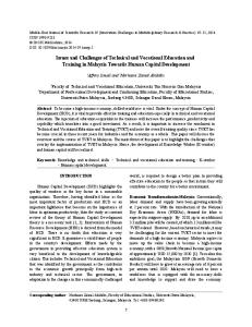


![Introduction [to Human Capital and Economic Development]](https://kipdf.com/img/300x300/introduction-to-human-capital-and-economic-develop_5afa94d68ead0ee4278b461c.jpg)