Growth and the World Economy Chapter 6
Outline � Convergence � Cross-Country Growth in the Long Run � The Augmented Solow Model � Geography, Institutions, and Growth
6.1 CONVERGENCE �In 1900, U.S. income per capita was 3.5 times larger than Japan and 6.6 times larger than India �In 2000, U.S. income per capita was only 1.3 times larger than Japan and 14.7 times larger than India �Why did the first gap narrow and the second gap widen?
6.1 CONVERGENCE �
Solow’s growth model production function: Y/N = F(K/N,1,A)
We assume that all countries have the same production function and access to technology: � If low level of capital per worker and low level of income per worker, then poor country � If high level of capital per worker and high level of income per worker, then rich country
6.1 CONVERGENCE Ex. In 1950 Y/N was lower in Japan than in U.S. What happened to the growth rates of these two countries? The U.S. is assumed to be at the steady state point but Japan seems to be to the left on the balanced growth path. This situation is not sustainable: over time K/N increases for Japan relative to the U.S. until it reaches the same steady state point as the U.S. Following this period the growth rates of the U.S. AND Japan are equal to each other and to the growth rate of technology.
6.1 CONVERGENCE The convergence hypothesis of Solow model: Over time, gaps in per-capita income among countries narrow. If the steady-state point is reached and the gap eliminated, the initially poorer country catches up with the initially richer country. After reaching the steady-state point, growth rates are equal with each other and the lines are identical.
- Question: How well does this hypothesis hold? It seems to hold for the U.S. and Japan. Does it hold for other countries?
Testing the Convergence Hypothesis Hypothesis: Growth rate of Y/N should be negatively related to the initial level of Y/N. Countries with low levels of Y/N should have higher growth rates.
Testing the Convergence Hypothesis Example: We have data for Y/N for 100 countries 1960-2000 - For each country compute the initial level and the annual growth rate of Y/N - Test convergence hypothesis:
∆(Y / N ) /(Y / N ) = a + c(Y / N )(1960) ∆ (Y / N ) /(Y / N ) = annual growth rate of Y/N c(Y / N )(1960) = initial level of Y/N
a = coeficient
Testing the Convergence Hypothesis Convergence hypothesis: c is negative – there is a negative relationship between the growth rate of GDP per capita and the initial level of GDP per capita
How well does the convergence hypothesis work?
Testing the Convergence Hypothesis �
�
Strong evidence of convergence among industrial countries since 1960 The evidence for convergence since 1960 does not extend to the world as a whole
Next two figures illustrate this fact:
Returns to Investment in Rich and Poor Countries � �
Important for the development of Endogenous Growth Theory Robert Lucas – had problems with Solow model.
Example: � Assume that average capital share in India and U.S. is 0.4 Y = K0.4N0.6A Divide by N: Y/N = A(K/N)0.4 �
If (Y/N in U.S.) = 15 (Y/N in India) and the countries have same technology – (K/N in U.S.) has to be 900 (K/N in India)
Returns to Investment in Rich and Poor Countries �The actual difference is about 20 �Therefore the returns to investment in India should be 58 times higher than the returns to investment in the U.S. �Solow model cannot answer the question “Why doesn’t capital flow from rich to poor countries?”
6.2 Cross Country Growth in the Long Run �What if we look at longer-term historical data? �Would the evidence for convergence among advanced countries and divergence among all the countries of the world still hold?
6.2 Cross Country Growth in the Long Run � Use data since 1900 � It includes advanced countries, Eastern
European, Latin American, Asian, and African countries � What do we find?
6.2 Cross Country Growth in the Long Run
� For 17 advanced countries - convergence, similar to post 1960’s data
� For the world - divergence:
�Countries that were poor in 1900 have grown slower than countries that were rich in 1900 �Income inequality has increased in the last century
The Future? �Rise in income inequality? �Demographic transition – gap between rich and poor will eventually narrow �Demographic transition has been completed in Europe �Africa – demographic transition still in progress (post Malthusian regime: income per capita growing but the population is growing faster)
Future? �Hope that a forthcoming transition for Africa will raise the 21st-century growth rates, as its modern growth regime begins �Problem: the AIDS epidemic – destroys human capital, lowers physical capital, and reduces population growth (AIDS has lowered the growth of GDP per capita in Africa by 0.5%/year)
Steady-State Growth - Solow model prediction – constant steady-state growth - Chapter 5. Remember, if we predict U.S. GDP/capita by extrapolating data from 1870 to 1929 (1929 is called a break date in US GDP/capita data) we would be off by only 19% - Does this long-run predictability extend beyond U.S.?
Steady-State Growth �
�
� �
Let’s illustrate the same thought experiment for Japan and the U.K.: predict GDP/capita in 2001 by extrapolating data following a break The break dates where the extrapolation begins are 1944 for Japan and 1918 for U.K. Very different results from the U.S. case The economist predicting GDP per capita would be off by 39% in the case of the U.K. and by 64% in the case of Japan
Constant Steady State Growth Hypothesis � How to evaluate this hypothesis? �Compare growth rates before and after break date �It work well for the U.S.: 1.8% before 1929 and 2% after 1929 �It does not work for the U.K. or Japan �This comparison overstates differences among countries: capital stock is destroyed (wars) and GDP per capita falls, followed by higher growth rates during the economy rebuilding
Constant Steady-State Growth Hypothesis Postwar transition period – time between the break and the year where the extrapolated growth line intersects the actual growth data (1958 for Japan and 1940 for the U.K.) Test the steady-state growth rate – compare the growth rates before the break and after the postwar transition period Result: There is no support for the prediction of constant steady-state growth
Constant Steady State Growth Hypothesis If we extend this analysis: This hypothesis holds only for Canada and U.S. Countries that behave like the U.K.: Finland and Sweden (WW1 – break date) Countries that behave like Japan: France and Germany (WW2 – break date) Does the Solow model hold then? We need to be careful about assuming constant steady-state growth across time.
6.3.The Augmented Solow Model �Two countries with different saving and laborforce growth rates move towards different steady-state levels of income per capita
�What does this tell us about testing for convergence?
6.3. The Augmented Solow Model �With the previous model, one would find convergence (with data starting from 1900) or even divergence (with data starting from 1800); the two countries have the same initial level of income per capita but one country has higher income per capita in 2000 (next figure) �Solow model does not work well when countries are not constrained to have the same steady state levels of per-capita income
6.3. The Augmented Solow Model �Test for conditional convergence - the hypothesis that income per capita in a given country converges to that country’s steady-state value �It implies that the initial level of income per capita is negatively related to the growth rate of income per capita after controlling for the saving rates and population-growth rates that determine the steady state
6.3. The Augmented Solow Model ∆(Y / N ) /(Y / N ) = a + c(Y / N )(1960) + (saving and population growth rates)
�If c is negative: �Provide evidence of convergence for the world
as a whole �Countries converge to their own steady state �It does not mean that the gap between rich and poor narrows
6.3. The Augmented Solow Model �Solow model predicts convergence when economies have the same saving rate and population-growth rate �Saving rates and population growth rates are similar among industrialized countries but not for not for the world as a whole.
6.3. The Augmented Solow Model � Allowing for countries to be in different steady states helps understand the nature of convergence; however, it does not eliminate all problems with the Solow model. � Problems: �When differences in income per capita are too large to be explained �When the speed of convergence is higher than predicted by Solow � When there are very large differences in rates of return to investment between rich and poor countries
Human Capital All of these led to the following development: the focus on human capital (H) in the development of the endogenous theory and in the augmented Solow model. Human capital = schooling and on-the-job training
Human Capital
� Production function that includes human capital: Y = F(K, H, N, L) = K1/3H1/3N1/3A Divide by N: Y/N = (K/N)1/3(H/N)1/3A
� Human capital accumulation proxy -- secondary school enrollment � Research finds that savings rates, population growth rates and human capital accumulation explains 78% in income differences
Augmented Solow Model with Human Capital � This model is used to investigate conditional convergence
∆(Y / N ) /(Y / N ) = a + c(Y / N )(1960) + (saving, population growth rates and human capital accumulation) � Initial level of income per capita is negatively related to growth rate of income per capita, after controlling for saving rates, population growth and humancapital accumulation
Augmented Solow Model with Human Capital � Share of physical and human capital is greater than the
share of capital in the original Solow model – it can help explain why the difference in capital per worker in rich and poor countries is not as large as would be predicted by Solow model � Assume average share of physical and human capital in India and US is 0.8, production function is: Y = K0.8N0.2A Divide by N: Y/N = A(K/N)0.8 K = both physical and human capital
Augmented Solow Model with Human Capital � Lucas question: If income per worker is 15 times higher in the U.S. than India, what is the physical and human capital per worker if the two countries have the same technology? � The answer: 30 (around 20 is the actual value observed), which is much lower than 900, predicted by the original model.
Cross Country Growth � What determines the differences in economic growth across countries? � We focus on conditional convergence
∆(Y / N ) /(Y / N ) = a + c(Y / N )(1960) + (saving, population growth rates and other var iables) � Conditional convergence - negative value of c coefficient
Cross Country Growth
�Equations – cross-country growth
regressions: variations in saving rates, population-growth rates, and other variables are used to explain growth �Examine the level of income across countries using cross-country level regressions.
Y / N = a + c(Y / N )(1960) + (saving, population growth rates and other var iables)
Cross Country Growth
� Some variables that can cause differences in growth
rates of income per capita or levels of income per capita among countries in cross country regressions: � Saving rates � Population growth � Measures of human capital � Political variables � Openness to trade � Market distortions � The fractions of primary products in total exports � Geographic variables
6.4. Geography, Institutions and Growth � Distance from the equator is highly correlated to income per capita. Countries far from the equator are relatively rich, and countries close to the equator are relatively poor. � What causes the relation between geography and income? � Does geography affect growth directly, or does the effect operate through social institutions?
Social Infrastructure Definition – the institutions and government policies that determine the economic environment within which individuals accumulate skills and firms accumulate capital and produce output � Differences in social infrastructure can explain much of the variation of levels of income per capita across countries beyond what can be accounted for by physical capital and human capital � Distance from the equator is a proxy for the influence of Western Europe, the first region to implement a social infrastructure favorable to production, on the rest of the world
Geography
The geography hypothesis: most of the differences in income per capita across countries can be explained by geographic, climatic, and ecological differences. � Tropical regions (centered near the equator) have grown at a slower rate than temperate regions (north or south of the tropics). Differences in the growth rates can be explained by: �Technological innovation being much higher in temperate climates than tropical regions. Yet, there is technological diffusion (technological innovation spreads to non-innovating countries). �Ecological divide seems to limit the degree to which technological innovation can spread.
Institutions The institutions hypothesis: differences in economic performance are caused by the organization of the society. � Geography influences growth through differences in institutions and social infrastructure among countries � Among European powers, there has been a reversal of fortune; when we use population density and degree of urbanization data as proxies for income per capita, regions that were relatively rich in 1500 are now relatively poor, and regions that were more densely populated in 1500 are now poorer than the ones that were more sparsely populated.