Joint International Conference on Computing and Decision Making in Civil and Building Engineering June 14-16, 2006 - Montréal, Canada

Geotechnical Data Mining Models (GDM) Using MS SQL2005 N. Nawari, Ph.D., P.E. 1

1

Kent State University, College of Architecture and Environmental Design, Kent, OH 44242 ……………

Abstract Geotechnical databases could be imprecise and multidimensional in nature; some hidden relationships within the data can only be retrieved using comprehensive data analysis techniques like data mining. Data mining employs algorithms that are a mixture of statistics, fuzzy logic, genetic algorithms, maths and artificial intelligence. There are a large number of algorithms that seek relationships within datasets from which rules of some kind can be derived and subsequently used for design prediction, classification or other functions, but selecting the most effective algorithm is not an intuitive process. The algorithms fall into a number of groups of methods where four of the most widely used are neural networks, decision trees, fuzzy and Baysian logic. This work is centred on experiments with algorithms provided by the new release of the Data Mining Tools for Microsoft SQL 2005 database server for predicting pile capacity from basic geotechnical data. Different data mining models in MS SQL2005 and in particular algorithms were chosen that were amongst the simplest examples of these groups of models, namely Association Rules, Decision Tree and Naïve Bayes, Clustering and Neural Network.

Introduction A database derived from geotechnical test results are normally noisy and contain multidimensional types of uncertainty. For design purposes, engineers used to establish relationships between some of the parameters in the data, which can be generated from empirical mathematical correlations or recognised by statistical methods. These relationships can then be used to make limited predictions of other unknown parameters from a few known values. In order to cope with such complexity of geotechnical behavior, and the spatial variability of the soil and rock materials, classical forms of engineering design models are justifiably reduced to simplified mathematical expressions. Recently some researchers (Chan, et.al (1995, Goh (1995; 1996), Lee (1996), Nawari et.al , 1999) have investigated the application of neural network to provide an alternative approach for geotechnical design and analysis. Their results were promising and indicated the potential of these techniques. However, most of the work cited deal with a limited data residing on flat structure. Nevertheless, as the databases would be imprecise and multidimensional in nature, some hidden relationships within the data can only be retrieved using comprehensive data analysis techniques like data warehousing and data mining. Data mining employs algorithms that are a mixture of statistics, fuzzy logic, genetic algorithms, maths and artificial intelligence. There are a large number of algorithms that seek relationships within datasets from which rules of some kind can be derived and subsequently used for design prediction, classification or other functions, but selecting the most effective algorithm is not an intuitive process. The algorithms fall into a number of groups of methods where five of the most widely used are neural networks, association rules, decision trees, fuzzy and Baysian logic. This work is centred on experimenting with algorithms provided by the new release of the Data Mining Tools for Microsoft SQL 2005 database server. The research illustrates the different data mining methods in MS SQL2005 and in particular algorithms were chosen that were amongst the simplest and practical for engineering design and analysis.

Basic Concepts Data mining is the process of extracting valid, authentic, and meaningful relationships from large quantities of data. It involves uncovering patterns in the data and is often tied to data warehousing because it attempts to make large amounts of data actionable. Data elements fall into distinct categories; these categories enable you to make predictions classifications about other pieces of data. For example, driven pile capacity can be assessed from a large amount of data about the soil profile, SPT, and pile tests. knowing soil profile and SPT attributes, engineers can use data mining to models to

Page 228

Joint International Conference on Computing and Decision Making in Civil and Building Engineering June 14-16, 2006 - Montréal, Canada

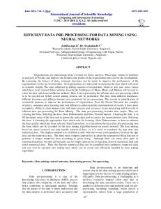
make predictions about the expected pile capacity. One of the more difficult aspects of applying data mining in engineering practice has always been translating the theory into routine techniques. An important concept is that building a mining model is part of a larger process that includes all from defining the basic problem that the model will solve, to deploying the model into a working environment. This process can be defined by using the following basic steps: - Define the problem - Preparing data - Defining models - Validation and exploration - Deploying and updating models The following diagram shows the steps involved in a typical data-mining project.

Define the model

Data Mining Manageme nt System

Training Train the model

Test Test the model

Data stores Predictions & classifying

Prediction Data

Figure 1. Data mining components The first step includes analyzing the requirements, defining the scope of the problem, defining the metrics by which the model will be evaluated, and defining the final objective for the data-mining project. These tasks can be summarized in the following: Defining the datasets for the analysis Identifying the attributes of the dataset that we want to try to predict What pattern and associations are we seeking? The second step involves the preparation, which may include calculating the minimum and maximum values, calculating mean and standard deviations, and looking at the distribution of the data. Microsoft SQL2005 server has a data Source View Designer in Business Intelligence(BI) Development Studio that contains several tools that allows such data exploration. Before defining the model data must be randomly separate into training and testing datasets. This step can be achieved by using the Percentage Sampling Transformation service available with SQL 2005 server as a part of the Integration Services. The Percentage Sampling transformation creates a sample dataset by selecting a percentage of the transformation input rows. The sample dataset is a random selection of rows from the transformation input, to make the resultant sample representative of the input. The training dataset is utilized to build the model, and the testing dataset to verify the accuracy of the model. A data mining model is typically defined by specifying input columns, an identifying column, and a predictable column. You can then define these columns in a new model by using the Data Mining Extensions (DMX) language,

Page 229

Joint International Conference on Computing and Decision Making in Civil and Building Engineering June 14-16, 2006 - Montréal, Canada

or the Data Mining Wizard in BI Development Studio all are available in SQL server 2005. This is known as mining structure that defines the data domain from which mining models are built. A single mining structure can contain multiple mining models that share the same domain. This structure contains information such as data type, content type, and how the data is distributed. After defining the structure of the mining model objects, training starts by populating the empty structure with the patterns that describe the model. Patterns are found by passing the original data through a mathematical algorithm. SQL Server 2005 contains different algorithms. The data mining algorithm is the mechanism that creates mining models. To create a model, an algorithm first analyzes a set of data, looking for specific patterns and trends. The algorithm then uses the results of this analysis to define the parameters of the mining model. In summary A mining model is defined by a data mining structure object, a data mining model object, and a data mining algorithm. Microsoft SQL Server 2005 Analysis Services (SSAS) provides several algorithms for use in data mining solutions: - Decisions Trees, Clustering, Association Rules, Naïve Bayes, and Neural Network The following is a simple illustration of these algorithms. Decisions Trees Decision tree is a classification and regression analysis for discrete or continuous attributes, the algorithm makes predictions based on the relationships between input columns in a dataset (Figure 2). It uses the values, or states, of those columns to predict the states of a column that is designated as predictable. Dataset

Decision Tree

Predictions Decision Rules

Figure 2. Decision Tree Diagram Association Rules Association rules algorithm is a mining mechanism for finding correlations between different attributes in a dataset. The most common application of this kind of algorithm is for creating association rules, which can be used in a forecast analysis. Association models are built on datasets that contain identifiers both for individual cases and for the items that the cases contain. A group of items in a case is called an itemset. An association model is made up of a series of itemsets and the rules that describe how those items are grouped together within the cases. The rules that the algorithm identifies can be used to predict a likely future value, based on the items that already exist in the dataset. The following diagram shows a series of rules in an itemset for predicting the axial pile carrying capacity: Rule

.

Depth50ft = 19, Depth15ft = 19 -> Capacity = 600 Perimeter = 113.1, Length = 68.050003 -> Capacity = 610.70001 Perimeter = 113.1, Depth70ft = 30 -> Capacity = 610.70001 Perimeter = 113.1, Depth65ft = 30 -> Capacity = 610.70001 Perimeter = 113.1, Depth55ft = 29 -> Capacity = 610.70001 Perimeter = 113.1, Depth45ft = 11 -> Capacity = 610.70001 Perimeter = 113.1, Area = 55.759998 -> Capacity = 610.70001 Perimeter = 113.1, Depth50ft = 29 -> Capacity = 610.70001 Perimeter = 113.1, Depth60ft = 29 -> Capacity = 610.70001 Perimeter = 113.1, Depth0ft = 3 -> Capacity = 610.70001 Perimeter = 113.1, Depth5ft = 3 -> Capacity = 610.70001 Perimeter = 113.1, Depth40ft = 3 -> Capacity = 610.70001 Perimeter = 113.1, Depth35ft = 3 -> Capacity = 610.70001 Perimeter = 94.25 -> Capacity = 606

Figure 3. An Example of Association Rules

Page 230

Joint International Conference on Computing and Decision Making in Civil and Building Engineering June 14-16, 2006 - Montréal, Canada

As the diagram illustrates, the Microsoft Association algorithm can potentially find many rules within a dataset. The algorithm uses two parameters, support and probability, to describe the itemsets and rules that it generates. For example, if X and Y represent two geotechnical parameters that could characterize the strength of soil, the support parameter is the number of cases in the dataset that contain the combination of items, X and Y. By using the support parameter in combination with the user-defined MINIMUM_SUPPORT and MAXIMUM_SUPPORT, parameters the algorithm controls the number of itemsets that are generated. The probability parameter, also called confidence, represents the fraction of cases in the dataset that contain X, that also contain Y. By using the probability parameter in combination with the MINIMUM_PROBABILITY parameter, the algorithm controls the number of rules that are generated. The Microsoft Association algorithm traverses a dataset to find items that appear together in a case. The algorithm then groups into itemsets any associated items that appear, at a minimum, in the number of cases that are specified by the MINIMUM_SUPPORT parameter. These rules are used to predict the presence of an item in the database, based on the presence of other specific items that the algorithm identifies as important. Naïve Bayes This algorithm calculates the conditional probability between input and predictable columns, and assumes that the columns are independent. It is based upon the simplifying hypothesis that when you evaluate column A as a predictor for target columns B1, B2, and son on, you can disregard dependencies between these target columns. This assumption of independence leads to the name Naive Bayes, with the assumption often being naive in that, by making this assumption, the algorithm does not take into account dependencies that may exist. This algorithm is less computationally intense than other algorithms, and therefore is useful for quickly generating mining models to discover relationships between input columns and predictable columns. Clustering The Microsoft Clustering algorithm is a segmentation algorithm provided that uses iterative techniques to group data cases into clusters that contain similar characteristics. These groupings are useful for exploring data, identifying anomalies in the data, and creating predictions. Clustering models identify relationships in a dataset that might not be derived logically through normal observation. This clustering differs from other data mining algorithms, such as the decision Trees algorithm, in that you do not have to designate a predictable column to be able to build a clustering model. The clustering algorithm trains the model strictly from the relationships that exist in the data and from the clusters that the algorithm identifies. The Microsoft Clustering algorithm first identifies relationships in a dataset and generates a series of clusters based on those relationships. A scatter plot is a useful way to visually represent how the algorithm groups data, as shown in the following diagram. The scatter plot represents all the cases in the dataset, and each case is a point on the graph. The clusters group points on the graph and illustrate the relationships that the algorithm identifies

Figure 4. Cluster groups diagram. Neural Network The Microsoft Neural Network algorithm creates classification and regression mining models by constructing a Multilayer Perceptron network of neurons. In this Multilayer Perceptron network, each neuron receives one or more inputs and produces one or more identical outputs. Each output is a simple non-linear function of the sum of the inputs to the neuron. Inputs only pass forward from nodes in the input layer to nodes in the hidden layer, and then finally they pass to the output layer; there are no connections between neurons within a layer. Similar to the Microsoft Decision Trees algorithm, the Neural Network algorithm calculates probabilities for each possible state of the input attribute when given each state of the predictable attribute. These probabilities can be used to predict an outcome of the predicted attribute, based on the input attributes.

Page 231

Joint International Conference on Computing and Decision Making in Civil and Building Engineering June 14-16, 2006 - Montréal, Canada

Data Inception The data selected for this work is stemming from test results on driven pile tests. The problem of determining the pile capacity from simple goetecnical tests like SPT-values or consistency limits is of a great interest in pile engineering. This problem has attracted many researchers and practioners over decades resulting in different solutions, known as pile driven formulas. Because of the complexity and the uncertainty space associated in the geotenical domain, no satisfactory solution or general procedure for estimating the pile capacity from simple soil tests is available. However, it is clear that certain relationship exists between the parameters involved in these formulas and the pile carrying strength. In summary, the enigma is a typical geotecnical problem that its solution should be derived from highly independent parameters, which are intrinsically noisy and error-prone. Data mining models offer a powerful tool in solving such problems. The database schema used for developing the mining models is shown in figure 3. This schema is designed to be flexible, simple, expandable, and adapt to any future changes and additions of basic geotechnical test data. The main focus of this work is to utilize a limited number of primary soil tests in the prediction model. Adding more input tables to the schema will enhance its performance in the prediction and classification process. For instance, additional results from the triaxial soil tests in terms of cohesion and angle of friction will extend the database schema with extra two dimensions tables. This will reduce the uncertainty level and provide an enriched mining model. The data used for this study is drawn from actual case records (Liang, 1998). For the purpose of the data mining analysis, the data is grouped into three categories: (i) Steel Pile (H-Section), (ii) Steel Piles (Pipe-Section), (iii) Pre-Stressed Concrete Piles There are 35 piles from group (i), 40 from group (ii) and 47 from group (iii).

Figure 5. Database Schema for Driven Piles.

Page 232

Joint International Conference on Computing and Decision Making in Civil and Building Engineering June 14-16, 2006 - Montréal, Canada

Analysis Microsoft Intelligence Development studio was used to create a project for the geotechnical data mining models (Figure 6). A number of steps are needed for the establishment of the models. These include: - Defining a data source: this is performed by referencing the pile database in MS SQL 2005 server. - Defining a data source view: A data source view provides an abstraction of the data source. This allows modifying the structure of the data to make it more relevant to specific projects. By using data source views, one can select the tables that relate to a particular project, establish relationships between tables, and add calculated columns and named views without modifying the original data source. - Investigate the attributes of the data that would affect the target parameter - Creating the mining structure which starts by defining the desired data mining technique Specifying the Training Data page (Figure 6) -

Figure 6: Definition of the training data The models built with this project are shown in figure 7. This include PC_Decision Tress mining model, PC_Clustering, PC_NaiveBayes, PC_Association_Ruels, and PC_NeuralNetwork mining models.

Figure 7. Pile capacity Mining Models in the Data Mining Designer

Figure 8. Clustering Model for Pile Capacity

The cluster diagram in figure 8 explores the relationship between the clusters that the algorthim discover for axial pile capacity. The lines between clusters represent “closeness” and are shaded based on how similar the clusters are.

Page 233

Joint International Conference on Computing and Decision Making in Civil and Building Engineering June 14-16, 2006 - Montréal, Canada

Figure 9: Definition of the Mining Model Prediction

Figure 10: Dependency Network of the Association Rules Model After testing the accuracy of your mining models and decided that you are satisfied with them, you can create Data Mining Extensions (DMX) prediction queries by using Prediction Query Builder on the Mining Model Prediction tab in Data Mining Designer. Data Mining Extensions (DMX) is a query language provided by Analysis Services that allow creating and working with mining models (figure 11). SELECT t.[Piletype], [PC_Neural_Network].[Capacity], PredictProbability([PC_Neural_Network].[Capacity]) From [PC_Neural_Network] PREDICTION JOIN OPENQUERY([Geotech Data], 'SELECT [Piletype], [Area], [Length], [Perimeter], [Depth0ft], [Depth5ft], [Depth10ft], [Depth15ft], [Depth20ft], [Depth25ft], Depth30ft], [Depth35ft], [Depth40ft], [Depth45ft], [Depth50ft], [Depth55ft], [Depth60ft], [Depth65ft], Depth70ft], [Depth75ft], Depth80ft], [Depth90ft], [Depth95ft], [Depth100ft], [Depth105ft], [Depth110ft], [Depth115ft], [Depth120ft], [Depth125ft] FROM [dbo].[vtest-H-Pile] ') AS t ON [PC_Neural_Network].[Area] = t.[Area] AND [PC_Neural_Network].[Length] = t.[Length] AND [PC_Neural_Network].[Perimeter] = t.[Perimeter] AND [PC_Neural_Network].[Depth0ft] = t.[Depth0ft] AND [PC_Neural_Network].[Depth5ft] = t.[Depth5ft] AND [PC_Neural_Network].[Depth10ft] = t.[Depth10ft] AND [PC_Neural_Network].[Depth15ft] = t.[Depth15ft] AND [PC_Neural_Network].[Depth20ft] = t.[Depth20ft] AND [PC_Neural_Network].[Depth25ft] = t.[Depth25ft] AND [PC_Neural_Network].[Depth30ft] = t.[Depth30ft] AND [PC_Neural_Network].[Depth35ft] = t.[Depth35ft] AND [PC_Neural_Network].[Depth40ft] = t.[Depth40ft] AND [PC_Neural_Network].[Depth45ft] = t.[Depth45ft] AND [PC_Neural_Network].[Depth50ft] = t.[Depth50ft] AND [PC_Neural_Network].[Depth55ft] = t.[Depth55ft] AND [PC_Neural_Network].[Depth60ft] = t.[Depth60ft] AND [PC_Neural_Network].[Depth65ft] = t.[Depth65ft] AND [PC_Neural_Network].[Depth70ft] = t.[Depth70ft] AND [PC_Neural_Network].[Depth75ft] = t.[Depth75ft] AND [PC_Neural_Network].[Depth80ft] = t.[Depth80ft] AND [PC_Neural_Network].[Depth90ft] = t.[Depth90ft] AND [PC_Neural_Network].[Depth95ft] = t.[Depth95ft] AND [PC Neural Network] [Depth100ft] = t [Depth100ft] AND [PC Neural Network] [Depth105ft] = t [Depth105ft] AND

Figure 11. An Example of SQL query used in the Neural Network Mining Mode

Page 234

Joint International Conference on Computing and Decision Making in Civil and Building Engineering June 14-16, 2006 - Montréal, Canada

Results and Discussion The measured axial pile capacities are compared with the capacities obtained by the data mining models during the testing phase. After accepting the performance of the prediction models, the data mining models are deployed on the analysis server and ready for new predictions. The Data Mining Models are then utilized to predict the pile capacity of a set of new data. The field test data represent SPT values and the pile geometric properties. Figures 12 to 14 present the measured pile capacities versus predicted by the different Data Mining Models. Figure 16 shows the regression surfaces for H-Piles generated. The best results of prediction are obtained by the Neural Network model and the Association Rules model. Both models have a correlation confident of 0.9 and higher, The Decision Tress and Naïve Bayes model performed poorly in the validation process. The Clustering Mining Model performs very well for the group of piles and indicates a correlation coefficient of 0.88.

Measured Pile Capacity (kips)

1400

Neural Network Decision Tree Clustering Association

1200 1000

Measured

800 600 400 200 0 0

200

400

600

800

1000

1200

140

Measured Pile Capacity (kips) Figure 12: Comparison of the Performance of Geotechnical Data Mining Models for H-Piles

The second group of data used to validate the data mining models is the steel pipe piles. The test results of total of 8 new piles are used to examine the performance of the models. Figure 17 depicts the result of the comparison between the different prediction algorithms. The performance of the Neural Network models shows a correlation coefficient of 0.93 whereas the Association Rules mining model indicate a value of 0.86 correlation coefficient. The Decision Tree and the Naïve Bayes models again achieve inadequate results in the prediction process of pile capacities when a new dataset is provided. The clustering discrimination algorithm attains an acceptable prediction performance with a correlation coefficient of 0.82. Comparable results are also obtained from the Prestressed Concrete Piles validation data plotted in figure 18. The performance of the Association Rules model indicates a correlation coefficient of 0.89, the Clustering model shows 0.90 whereas Neural Network algorithm denotes 0.92.

Page 235

Joint International Conference on Computing and Decision Making in Civil and Building Engineering June 14-16, 2006 - Montréal, Canada

1000 NN

Predicted Pile Capacity (kips)

Dtree Clustering

800

Association Measured

600

400

200

0 0

200

400

600

800

1000

Measured Pile Capacity (kips)

Figure 13: Performance Comparison of the Geotechnical Data Mining Models for Steel Pipe-Piles

1000

Neural Network Decision Tree

900

Clustering Predicted Pile Capacity (kips)

800

Association Measured

700 600 500 400 300 200 100 0 0

100

200

300

400

500

600

700

800

900

Measured Pile Capacity (kips)

Figure 14: Performance of the DMM for Prestressed-Piles

Page 236

1000

Joint International Conference on Computing and Decision Making in Civil and Building Engineering June 14-16, 2006 - Montréal, Canada

Conclusions The efficiency of the modeling methods describing the response of the soil-structure system depends to a large extends on the ability to specify the relevant geotechncial characteristics data. Soil properties vary widely at a given site and the limitations of current sampling and testing techniques intensify this variation. Data Mining Techniques are alternative approaches that can encapsulate the variability in soil properties and interactions. The current paper focuses on experimenting with data mining algorithms performance with respect to varying geotechnical data and consequently provides suggestions for the most appropriate data-mining model for goetechnical design and analysis. Data Mining Tools specified in Microsoft SQL 2005 database server are utilized for this study. The five data mining models investigated are Decision Tree, Naïve Bayes, Clustering, Association Rules, and Neural Network. According to these mining models test results assert the feasibility of the approach. Namely, the Clustering, Association Rules and the Neural Network mining models indicate a great potential to approximate the axial pile capacity of full-scale pile test results. The models utilize simple soil tests as input dimensions. In this study only SPT-test results are incorporated.. The performance of these mining models can be enhanced further in two ways. First as more data is accumulating into the database store, the finer the prediction capability of the models. In this manner, as the test data collection progresses through time, the data mining process refines the information gathered from its operating procedure. Second, by introducing more simulation input dimensions such as liquid limit, plasticity index, specific gravity, and moisture content will perceptibly furnish an increased prediction performance. Once this series of data mining models defined and refined in a loop process are reliable and produce consistent results, they can then serve as a component of an engineering decision making process integrated within the classical design and analysis process.

References Chan, W.T., Chow, Y.K. and Liu, L.F., (1995). "Neural Network: An alternative to pile driving formulas". Computers and Geotechnics, Elsvier, Amsterdam, 135-156. Goh, A. T. C. (1995). “Empirical design in geotechnics using neural networks.” Geotechnique, 45(4), 709-714. Goh, A. T. C. (1996b). “Pile driving records reanalyzed using neural networks.” J. Geotech. Engrg., ASCE, 122(6), 492-495. Liang, R., 1998, "Development and Implementation of New Driven Piles Technology", The Ohio Department of Transportation and the US Department of Transportation, Federal Highway Administration. Lee, I. M., and Lee, J. H. (1996). “Prediction of pile bearing capacity using artificial neural networks.” Computers and Geotechnics, 18(3), 189-200. Microsoft Corporation (2005). “SQL Server 2005 Book online”, Microsoft Corp., One Microsoft Way, Redmond, WA 98052-6399 Nawari, N. O., Liang, R. and Nusirat, J (1999) . “Artificial Intelligence Techniques for the Design and Analysis of Deep Foundations”. Electronic Journal of Geotechnical Engineering, Vol.4.

Page 237