Finite Element Analysis of Knee Cartilage with an Osteochondral Graft

A Thesis

Presented in Partial Fulfillment of the Requirements to Graduate with Distinction in Mechanical Engineering

By William Bogatay

The Ohio State University 2009

Approved by: _________________________ Dr. Noriko Katsube Faculty & Research Advisor Dept. of Mechanical Engineering

Abstract

Arthritis is the debilitating condition of deteriorated joint cartilage brought on by injury or normal wear over time. Many forms of treatment for knee arthritis are available based on the age and condition of the patient. One treatment option for patients is osteochondral grafting. Cylindrical grafts of bone and cartilage are taken from a donor site that experiences relatively minimal stress and inserted at the location of deteriorated cartilage. The project investigated the effect of graft depth and graft cartilage stiffness on stress distribution in knee cartilage. The investigation was accomplished through the use of an idealized axisymmetric finite element analysis. A graft depth changes of 1 mm resulted in an increase in cartilage contact stress as high as 83% and an increase in maximum cartilage shear stress as high as 150%. Small variation of the graft cartilage stiffness did not result in a dramatic change in contact pressure or shear stress. Although the investigations showed the relative effect of improper graft depth, the operation remains viable because it decreases pain in the short-term and extends the timeframe for the patient’s active lifestyle.

ii

Acknowledgements

Dr. Noriko Katsube – Who continued to patiently advise my project despite my on/off co-op schedule. Dr. Yaou Wang – Without whom I would have been lost when working with Abaqus.

iii

Table of Contents Abstract .................................................................................................................................................... ii Acknowledgements................................................................................................................................. iii List of Tables............................................................................................................................................. v List of Figures .......................................................................................................................................... vi 1. Introduction ............................................................................................................................................. 1 1.1 Treatment Options ............................................................................................................................. 1

2. Methods ................................................................................................................................................... 3 2.1 Preliminary Model Description .......................................................................................................... 3 2.2 Analytical Solution for Preliminary Models ....................................................................................... 5 2.3 Preliminary Verification Results ......................................................................................................... 6 2.4 Graft Depth and Material Model Descriptions ................................................................................ 10 3. Results .................................................................................................................................................... 12 3.1 Graft Depth Investigation Results .................................................................................................... 12 3.2 Graft Cartilage Material Investigation Results ................................................................................. 17 4. Conclusion .............................................................................................................................................. 24 5. Recommendation................................................................................................................................... 26

Bibliography ................................................................................................................................................ 27

iv

List of Tables Table 2.1: Comparison between analytical and finite element results for bone and cartilage cases. ......... 9 Table 2.2: Contact area radius compared to overall size for bone and cartilage cases. .............................. 9 Table 3.1: Contact stress results summary for graft depth investigation................................................... 14 Table 3.2: Tresca stress results summary from graft depth investigation. ................................................ 17 Table 3.3: Contact stress results summary for material investigation. ...................................................... 19

v

List of Figures Figure 1.1: Labeled knee with grafts ............................................................................................................. 2 Figure 2.1: Bone-on-bone properties and settings on unmeshed and meshed model ................................ 4 Figure 2.2: Deformation comparison between bone and cartilage models ................................................ 6 Figure 2.3: Contact stress and z-displacement for the bone verification case. ............................................ 7 Figure 2.4: Contact stress and z-displacement for the cartilage verification case. ...................................... 8 Figure 2.5: Model diagram for graft depth and material investigations .................................................... 11 Figure 3.1: Contact stress for various graft depths..................................................................................... 13 Figure 3.2: Tresca stress contour comparison for control and 1 mm depression. ..................................... 14 Figure 3.3: Tresca stress contour comparison for control and 0.5 mm depression. .................................. 15 Figure 3.4: Tresca stress contour comparison for control and flush graft. ................................................ 15 Figure 3.5: Tresca stress contour comparison for control and 0.5 mm protrusion. ................................... 16 Figure 3.6: Tresca stress contour comparison for control and 1 mm protrusion. ...................................... 16 Figure 3.7: Contact stress for the flush graft case with graft cartilage stiffness comparison. ................... 18 Figure 3.8: Tresca stress contour comparison for graft cartilage E = 5 MPa and E = 4 MPa. ..................... 19 Figure 3.9: Tresca stress contour comparison for graft cartilage E = 5 MPa and E = 4.5 MPa. .................. 20 Figure 3.10: Tresca stress contour comparison for graft cartilage E = 5 MPa and E = 4.75 MPa. .............. 20 Figure 3.11: Tresca stress contour comparison for graft cartilage E = 5 MPa and E = 5.25 MPa. .............. 21 Figure 3.12: Tresca stress contour comparison for graft cartilage E = 5 MPa and E = 5.5 MPa. ................ 21 Figure 3.13: Tresca stress contour comparison for graft cartilage E = 5 MPa and E = 6 MPa. ................... 22 Figure 3.14: Effect of cartilage stiffness on contact stress with a graft protrusion .................................... 23

vi

1. Introduction Cartilage plays an extremely important role within the body’s joints; in the case of the knee, it facilitates motion by lubricating the surfaces of the tibia and femur. The coefficient of friction in a healthy joint is “one-fifth of that between two pieces of ice” [1], but there is significantly more friction, and therefore pain, in a joint with deteriorated cartilage. Unfortunately, cartilage does not repair itself as well as other entities in the body and is very susceptible to damage. The damage can be accelerated by injuries to ligaments and menisci. Patients that suffer from damaged cartilage could benefit from advances made in treatment.

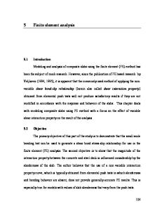
1.1 Treatment Options A viable treatment option for older, less active patients with severe cartilage damage is joint replacement, but this is not the case for younger patients. Replacement joints cannot handle large amounts of stress and will ultimately fail, resulting in further complications and surgeries. Therefore many doctors and scientists have spent their time developing procedures to repair articular cartilage, allowing active patients to eventually resume their lifestyles relatively pain-free. Microfracture surgery, which aims to stimulate blood flow and promote regeneration, is a popular procedure for young patients but it is not performed on patients in their forties or fifties. A surgical procedure that can help such a patient is osteochondral autograft replacement. Grafts are taken from a part of the knee that experiences relatively little stress and then transplanted to the area with deteriorated cartilage. This reduces pain in the knee because nerves in the subchondral bone in areas of high stress are no longer exposed. Figure 1.1 shows a labeled knee with example graft donor and recipient sites.

Figure 1.1: Labeled knee with grafts (adapted from [2]).

There are detriments to the osteochondral grafting procedure. Errors in graft placement can occur in surgery and graft cartilage may not perfectly match the native cartilage it replaces. Stress distribution could be affected by the depth of graft placement or graft cartilage material properties. A way to investigate the stress distribution caused by osteochondral grafting is finite element analysis (FEA). Although there are accuracy limitations, a well-developed model can provide a good estimate of stress in the knee. Parameters can be changed easily, and an indefinite number of simulations can be run which allows trends to be observed. The model can be updated and refined in order to conduct more realistic and accurate analyses.

2

2. Methods A simplified model of the knee was used to analyze the effects of plug depth and plug material on stress distribution. The model ignored ligaments and menisci, thus consisting of only bone and cartilage. Both materials were modeled as linear elastic. Prior to the bone-cartilage analyses, preliminary analyses had to be conducted. Analytical solutions can be used to verify stress and displacement between elastic bodies in contact. When each body is composed of more than one material (e.g. bone with a layer of cartilage) the effective stiffness of each body changes and the equations cannot be used. Therefore models consisting of only bone and only cartilage were simulated to verify the general contact problem. This provides a level of confidence in subsequent simulations despite the lack of an analytical solution involving multiple materials. The finite element software package Abaqus was used to conduct the study. ANSYS had been used briefly until difficulties were encountered when finding solutions for contact problems. Abaqus presented fewer difficulties and a friendlier user interface and therefore was selected.

2.1 Preliminary Model Description A model consisting of bone, shown in Figure 2.1, was analyzed first. The model was twodimensional axisymmetric with femur and tibia surface radii of 50 and 100 mm, respectively. The base of both the femur and tibia was 20 mm, which is an arbitrary size. The “cartilage” thickness was 2 mm [3]. Cartilage sections were incorporated because material modification is a relatively simple process in the software; subsequent analyses were facilitated by the presence of these sections. In the all-bone case, the cartilage sections (Sections 2 and 3 in Figure 2.1) as well as the bone sections (Sections 1 and 4) were given linear elastic bone material properties: E = 5 GPa, ν = 0.3 [4]. Two boundary conditions were applied to the model; the axis of symmetry of the model was fixed in the r-direction and the bottom of the model was fixed in the z-direction (the coordinate system can be seen in Figure 2.1). An equivalent load of 375 N was applied as a pressure of ~3 MPa at the top 3

of the femur, which created an evenly distributed loading condition. A load of 375 N is roughly half of an average human’s body weight. Quadratic (8-node), quadrilateral elements were used in the model and were meshed in a structured manner. Sections 2 and 3 had a slightly finer mesh, but mesh optimization was not yet an issue so the entire model’s mesh is generally fine. A surface-to-surface contact interaction was applied to Sections 2 and 3. The normal behavior was set to hard contact, which attempts to minimize surface penetration. The tangential behavior was set to frictionless. The small sliding setting was used, which defines how nodes interact with surfaces. The surface of Section 2 was the master while the surface of Section 2 was the slave because the master must be the surface that initiates contact.

Figure 2.1: Bone-on-bone properties and settings on unmeshed and meshed model. Sections 1-4 were created to facilitate subsequent modeling; in this case, all four sections are modeled as bone.

4

An identical analysis, with the exception of material property, was run for the cartilage-oncartilage case. Sections 1-4 were changed to a linear elastic cartilage model, with E = 5 MPa and ν = 0.46 [4].

2.2 Analytical Solution for Preliminary Models Hertz pressure “is exerted between two frictionless elastic solids of revolution in contact”. Hertz pressure as well as displacement in the z-direction was used to verify the preliminary bone-bone and cartilage-cartilage models. From [5]: 1/3

 3PR  a=   4E ' 

(1)

, contact area radius

With point load P and:

1 1 1 , effective radius of curvature = + R RFemur RTibia

 1 −ν 2  1 = 2 , E'  E 

(2) ( 3)

effective stiffness

Maximum pressure is given by:

p0 =

3P , 2π a2

maximum contact pressure

(4)

The following equations allow the calculation of Hertz (i.e. contact) pressure and z-displacement as a function of distance along the target body surface:

p(L) p0 1 − ( L / a ) , = 2

Hertz pressure distribution

1 −ν 2 π p0 2a2 − L2 ) , UZ ( L ) = ( E 4a

Z-displacement, L ≤ a

5

( 5) (6)

1/2  a2   1 −ν 2 p0  2 2 −1  a  UZ ( L ) = ( 2a − L ) sin   + ar  1 − 2   , E 2a  L  L   

Z-displacement, L > a

(7)

2.3 Preliminary Verification Results Figure 2.2 shows the post-analysis undeformed and deformed models of the bone and cartilage Hertz contact verification. The data path (variable L) used to verify the finite element result against the analytical result is shown on the undeformed model for the bone case. The cartilage case required a longer data path because the model deformed substantially. Bone did not deform nearly as much as cartilage due to higher stiffness.

Figure 2.2: Deformation comparison between bone and cartilage models. The data path used for contact stress and displacement plots in the bone model is called out on the undeformed model. The cartilage required a longer data path.

6

Contact Pressure, Bone

Stress Z-Z (MPa)

0

-20

-40

-60

-80

0

1

2

3

6 5 4 Data Path L (mm)

7

8

9

10

Z-displacement, Bone 0 -0.005

z

U (mm)

-0.01 -0.015 -0.02 -0.025 Analytical FEA

-0.03 -0.035

0

1

2

3

6 5 4 Data Path L (mm)

7

8

9

10

Figure 2.3: Contact stress and z-displacement for the bone verification case.

Figure 2.3 shows contact stress and displacement (both in the z-direction) plotted against radius, which was taken from the data path. Qualitatively the finite element result for bone contact sufficiently matches the analytical result obtained with the Hertz equations. The high stiffness of bone resulted in high stress over a small contact area. The finite element contact stress follows the parabola given by the analytical solution. Although small, the displacement given by the finite element analysis also follows the curve of the analytical solution with a little amount of error. 7

Contact Pressure, Cartilage 0.2

Stress Z-Z (MPa)

0 -0.2 -0.4 -0.6 -0.8 -1

0

2

4

6

12 10 8 Data Path L (mm)

14

16

18

20

Z-displacement, Cartilage 0 -0.5

z

U (mm)

-1 -1.5 -2 -2.5 Analytical FEA

-3 -3.5 0

2

4

6

12 10 8 Data Path L (mm)

14

16

18

20

Figure 2.4: Contact stress and z-displacement for the cartilage verification case.

As seen in Figure 2.4, the finite element result for the cartilage case did not agree with the analytical solution as well as the bone case. The finite element contact pressure tended towards the analytical solution as radius increased, but some error existed at the axis of symmetry. The finite element displacement curve was similar to but offset from the analytical displacement curve. The contact area radius of the cartilage model, as seen in the contact pressure plot (Figure 2.4) and the

8

deformed model (Figure 2.2), was much larger than that of the bone model due to the lower stiffness of cartilage. Additionally, stresses were lower in the cartilage case than the bone case. Table 2.1: Comparison between analytical and finite element results for bone and cartilage cases. The maximum values shown occur at the axis of symmetry.

Bone: E = 5 GPa, ν = 0.3 Analytical Finite Element % Difference Max Contact Stress (MPa) 78.99 79.02 0.03% Max Z-displacement (mm) 0.0340 0.0326 4.12% Cartilage: E = 5 MPa, ν = 0.46 Analytical Finite Element % Difference Max Contact Stress (MPa) 0.869 0.953 9.68% Max Z-displacement (mm) 3.09 2.47 19.96% Table 2.1 quantitatively compares the finite element results with the analytical values for bone and cartilage. Maximum contact stress and maximum displacement are shown. The differences between finite element and analytical values for the bone-bone case are within 5%, which is acceptable. The maximum contact stress for the cartilage-cartilage case, however, is different by nearly 10%, and the displacement is different by almost 20%. Further review of the Hertz contact equations and their underlying assumptions [5] revealed crucial details that justify the finite element result in the cartilage case. The analytical solution assumes that contact area radius is much smaller than radii of curvature and overall geometries. Table 2.2 summarizes the size of contact area radius relative to effective radius of curvature and model width for both bone and cartilage. In the case of bone, contact area radius is much smaller than overall geometry. In the case of cartilage, contact area radius is not much smaller than overall geometry. It is 43% of radius of curvature and 72% of width. Table 2.2: Contact area radius compared to overall size for bone and cartilage cases.

Analytical Contact Effective Radius Section Area Radius, a (mm) of Curvature, R (mm) Width, w (mm) Ratio a/R (%) Ratio a/w (%) Bone 1.51 33.33 20 4.5% 7.5% Cartilage 14.4 33.33 20 43.1% 71.8%

9

The analytical solution cannot be applied to the cartilage case directly because the material results in a large contact area radius. Nonetheless, the cartilage verification is encouraging because the curves are similar to the would-be analytical result. The specific values of the finite element result are likely more accurate than the analytical values because the cartilage case violates the assumptions used with the Hertz result. Regardless of the cartilage case outcome, the bone cased undoubtedly verifies the analysis.

2.4 Graft Depth and Material Model Descriptions A model to investigate the effect of graft depth on stress distribution was developed after preliminary verification. Figure 2.5 shows several modifications made to the previous model. Sections 1, 4 and 5 were modeled as bone while Sections 2, 3, and 6 were modeled as cartilage. The graft itself was 15 mm long with a radius of 3.5 mm. Five cases were investigated – graft depressions of 0.5 and 1 mm, protrusions of 0.5 and 1 mm, and a graft flush with the other femur cartilage (the ideal case). Figure 2.5 shows the 1 mm protrusion. A contact interaction between the plug and the femur was added, which included a friction coefficient of 0.3 (the cartilage contact interaction remained frictionless). The mesh was altered to be finer near the areas of interest, specifically near the graft surface. Due to software issues the femur bone had to be meshed freely (i.e. non-structured). A thermal isotropic expansion was conducted before load application in order to create an interference press fit of 1% for the graft [5]:

∆r =γ∆T =0.01 r Arbitrarily setting ∆T = 20 and solving for the expansion coefficient yielded γ = 0.0005. Thus, the expansion coefficient γ and a temperature field ∆T were applied to the graft in order to create a 1% interference fit. A 100 N load was applied as a pressure of 0.8 MPa in the step following the thermal expansion. 100 N is a close approximation of the load experienced by cartilage during post-operation 10

continuous passive motion [6]. Continuous passive motion is used after surgeries to apply a small amount of stress on the knee; a machine moves the knee on the order of one cycle per minute. A simulation was also conducted with a “healthy” knee, where there was no hole or graft. Essentially it was the same model as the verification simulations, but Sections 1 and 4 (Figure 2.1) were modeled as bone and Sections 2 and 3 as cartilage. This simulation served as a control. A material investigation was conducted after the graft depth investigation. The flush, or ideal, graft case was used and the modulus of elasticity of the graft cartilage (Section 6 in Figure 2.5) was varied ±5%, ±10%, and ±20%.

Figure 2.5: Model diagram for graft depth and material investigations. Dimensions and boundary conditions are unchanged from Figure 2.1 unless noted.

11

3. Results Two results were obtained in both the graft depth and material investigations: contact stress on the tibia surface and Tresca stress contour plots with limits that allowed cartilage shear stress to be analyzed. Contact stress data was collected with a data path, just as in the verification analyses. It shows which parts of the knee cartilage are being under- and over-utilized. Tresca theory is also known as the maximum-shear-stress theory [7]. Shear stress can be damaging to cartilage, and thus should be reported.

3.1 Graft Depth Investigation Results Figure 3.1 shows the tibia cartilage contact stress for each graft depth plotted with the control simulation, which was a healthy knee with no hole or graft. As the graft proceeds from depressed (Graph a) to protruded (Graph e), the contact stress in the graft region increases, while the contact stress elsewhere decreases. Unlike the healthy knee, each case results in an undesirable shift in contact pressure at the point where the graft and native cartilage meet. Change in geometry results in stress concentrations which, depending on severity, could damage cartilage in either the graft or the native cartilage. For example Table 3.1 shows that the 1 mm protrusion resulted in a maximum contact stress at the axis of symmetry that was 83% higher than the maximum contact pressure in the healthy knee. Even the ideal case of a flush graft resulted in a maximum contact pressure that was 12% higher than the healthy knee case. Alternatively a lack of stress could be just as detrimental as an abundance of stress. Tissues in the body break down when unused. Continuous passive motion is used in rehabilitation shortly after joint surgeries because stress is necessary to maintain or strengthen tissue [1]. Although the maximum contact stress in the depressed grafts was smaller than that of the healthy knee, it was discontinuous. In the case of the 1 mm depression, there was nearly zero contact pressure on the graft cartilage. The graft did not carry any load. Additionally the graft created a stress concentration in the native cartilage. 12

-1 mm (Depression)

-0.5 mm (Depression) 0.5 Contact Pressure (MPa)

Contact Pressure (MPa)

0.5 0 -0.5 -1 -1.5 -2 -2.5 -3 0

2 4 6 (a) Data Path L (mm)

0 -0.5 -1 -1.5 -2 -2.5 -3

8

0

0.5

0

0

-0.5 -1 -1.5 -2 -2.5 -3 0

2 4 6 (c) Data Path L (mm)

8

+0.5 mm (Protrusion)

0.5 Contact Pressure (MPa)

Contact Pressure (MPa)

0 mm (Flush Graft)

2 4 6 (b) Data Path L (mm)

-0.5 -1 -1.5 -2 -2.5 -3

8

0

2 4 6 (d) Data Path L (mm)

8

+1 mm (Protrusion) Contact Pressure (MPa)

0.5 0 -0.5

Healthy Knee (same for all cases) Knee with Graft Edge of Graft

-1 -1.5 -2 -2.5 -3 0

2 4 6 (e) Data Path L (mm)

8

Figure 3.1: Contact stress for a) 1 mm depression, b) 0.5 mm depression, c) 0 mm flush graft, d) 0.5 mm protrusion, and e) 1 mm protrusion. All plots contain the graftless, holeless control simulation and a marker signifiying the edge of the graft.

13

Table 3.1: Contact stress results for graft depth investigation.

Graft Depth Healthy knee Healthy knee 1 mm depression 0.5 mm depression 0 mm (flush) 0.5 mm protrusion 1 mm protrusion

Contact Pressure (MPa) 1.05 1.65 1.31 1.23 1.85 2.58 3.03

Location Femur Hole Edge Axis of Symmetry Femur Hole Edge Femur Hole Edge Axis of Symmetry Axis of Symmetry Axis of Symmetry

% Increase from Healthy Knee 0.0% 0.0% 24.8% 17.0% 12.1% 56.0% 83.1%

Figures 3.2 through 3.6 show Tresca stress contour plots for the various graft depths. The first plot is the control, or healthy knee. The second plot is the knee with the osteochondral graft. Higher stresses were observed in the graft and femur bone due to the press fit and stiff properties, but the investigation was concerned with cartilage stress; therefore the contour limits were set such that cartilage stresses could be observed. The limits of the control plot were identical to the limits of the corresponding graft plot, e.g. both plots of Figure 3.2 had an upper limit of 1.75 MPa and lower limit of 0 MPa. This allowed relative comparison between the healthy and surgically repaired knees.

Figure 3.2: Tresca stress contour comparison for control and 1 mm depression.

14

Figure 3.3: Tresca stress contour comparison for control and 0.5 mm depression.

Figure 3.4: Tresca stress contour comparison for control and flush graft.

15

Figure 3.5: Tresca stress contour comparison for control and 0.5 mm protrusion.

Figure 3.6: Tresca stress contour comparison for control and 1 mm protrusion.

16

The depression cases (Figures 3.2 and 3.3) showed a shear stress concentration where the femur cartilage got trapped between the graft cartilage and tibia cartilage, in contrast to the even stress distribution of the healthy knee. The stress concentration was more severe in the 1 mm depression than the 0.5 mm depression. The flush graft (Figure 3.4) resulted in a similar stress distribution to the healthy knee. The graft itself sees slightly more stress than the corresponding area in the healthy knee, however. Finally the highest shear stresses were seen in the protrusion cases (Figures 3.5 and 3.6), with the 1 mm protrusion being most severe. These stress concentrations occurred in large portions of the graft cartilage. Table 3.2 summarizes the results of the Tresca stress contour plots and compares the maximum values to the healthy knee case. Table 3.2: Tresca stress results from graft depth investigation.

Graft Depth Healthy knee 1 mm depression 0.5 mm depression 0 mm (flush) 0.5 mm protrusion 1 mm protrusion

Tresca Contour Upper Limit (MPa) 1.00 1.75 1.50 1.00 2.00 2.50

Location of Max Tresca Stress Tibia Cartilage Femur Cartilage Femur Cartilage Tibia Cartilage Graft Cartilage Graft Cartilage

% Difference from Healthy Knee 0% 75% 50% 0% 100% 150%

3.2 Graft Cartilage Material Investigation Results Figure 3.7 shows the contact stress along the tibia cartilage surface for varying graft cartilage material cases. The graft position is flush with femur. The range for Young’s modulus for the graft cartilage was ±20% of the original Young’s modulus, which was 5 MPa. Each varying stiffness case was plotted with the original case, and as the graphs show, graft cartilage material did not have a significant effect on contact stress in comparison to the plug depth contact stress. Table 3.3 shows the maximum contact stresses, which occurred at the axis of symmetry, for each graft cartilage modulus. Lower moduli resulted in lower maximum stress and higher moduli resulted in higher maximum stress, but the percent changes due to the altered graft cartilage moduli are low.

17

E = 4 MPa

Graft Cartilage E = 5 MPa Graft Cartilage E Varies

-0.5

-1

-1.5

-2

0

2 4 6 (a) Data Path L (mm)

-0.5

-1

-1.5

-2

8

0

E = 4.75 MPa Contact Pressure (MPa)

Contact Pressure (MPa)

-1

-1.5

0

2 4 6 (c) Data Path L (mm)

-0.5

-1

-1.5

-2

8

0

E = 5.5 MPa

2 4 6 (d) Data Path L (mm)

8

E = 6 MPa

0

0 Contact Pressure (MPa)

Contact Pressure (MPa)

8

E = 5.25 MPa

-0.5

-0.5

-1

-1.5

-2

2 4 6 (b) Data Path L (mm)

0

0

-2

E = 4.5 MPa

0 Contact Pressure (MPa)

Contact Pressure (MPa)

0

0

2 4 6 (e) Data Path L (mm)

-0.5

-1

-1.5

-2

8

0

2 4 6 (f) Data Path L (mm)

8

Figure 3.7: Contact stress for the flush graft case along the tibia cartilage surface and graft cartilage E = a) 4 MPa, b) 4.5 MPa, c) 4.75 MPa, d) 5.25 MPa, e) 5.5 MPa, and f) 6 MPa. Each are plotted against the standard case of E = 5 MPa.

18

Table 3.3: Contact stress results for material investigation.

Graft Cartilage Modulus (MPa) 4.00 4.50 4.75 5.00 5.25 5.50 6.00

Maximum Contact Stress (MPa) 1.82 1.89 1.92 1.94 1.97 2.00 2.04

% Difference in Max Stress -6.1% -2.7% -1.1% 0.0% 1.7% 3.0% 5.4%

Figures 3.8 – 3.13 show Tresca stress contour plots comparing the original graft cartilage to the modified cartilage. Unlike the previous contour plots, the upper limit for each plot is the same – 1 MPa. The Tresca stress results were similar to the contact stress results. The shear stress did not change drastically as Young’s modulus of graft cartilage changed.

Figure 3.8: Tresca stress contour comparison for graft cartilage E = 5 MPa and E = 4 MPa.

19

Figure 3.9: Tresca stress contour comparison for graft cartilage E = 5 MPa and E = 4.5 MPa.

Figure 3.10: Tresca stress contour comparison for graft cartilage E = 5 MPa and E = 4.75 MPa.

20

Figure 3.11: Tresca stress contour comparison for graft cartilage E = 5 MPa and E = 5.25 MPa.

Figure 3.12: Tresca stress contour comparison for graft cartilage E = 5 MPa and E = 5.5 MPa.

21

Figure 3.13: Tresca stress contour comparison for graft cartilage E = 5 MPa and E = 6 MPa.

One additional analysis was performed to determine if there is a significant interaction between plug depth and plug cartilage stiffness. Figure 3.14 shows the contact stress with a 1 mm graft protrusion for graft cartilage E = 4, 5, and 6 MPa. The curves are nearly identical. The effect of graft cartilage stiffness on cartilage stress is small in the flush graft case, but it is even smaller with the 1 mm protrusion.

22

Graft Cartilage Stiffness Study with 1 mm Protrusion 0.5

Contact Pressure (MPa)

0

-0.5

-1

-1.5

-2 E = 5 MPa E = 4 MPa E = 6 MPa

-2.5

-3 0

1

2

5 4 3 (a) Data Path L (mm)

6

7

Figure 3.14: Effect of cartilage stiffness on contact stress with a graft protrusion

23

8

4. Conclusion Arthritis is a debilitating condition that affects the quality of life as humans are injured or aging. When cartilage is gone in a middle-aged or elderly patient, it is not likely to return, and an active lifestyle is no longer a reality. Osteochondral grafting is a surgical treatment option that can reduce the ill effects of deteriorated cartilage and prolong active lifestyles. Finite element analyses were conducted to study these effects. Preliminary knee models were analyzed with finite elements; the bone model was verified with Hertz contact equations while the cartilage model violated assumptions made by the equations. Nonetheless, the cartilage results were similar enough to Hertz analytical results that the model was verified. A model with a press-fit graft was then created and modified two ways. First the graft depth was altered, and then the graft cartilage material properties were altered. Graft depth is a significant factor in the stress distribution in knee cartilage whereas graft cartilage material stiffness has relatively little effect. The contact stress and the Tresca shear stress were greatly dependent on graft depth. If the graft surface was just 1 mm below the femur surface, the graft did not make contact with the tibia cartilage under a 100 N load and harmfully high shear stresses were exhibited in the adjacent femur cartilage. If the graft surface protruded from the femur surface by just 1 mm, abnormally high contact and shear stresses were seen in the graft cartilage, potentially causing serious damage to the replacement cartilage. Although better than the 1 mm cases, the 0.5 mm depression and protrusion produced contact and shear stresses that could potentially damage cartilage. Based on the finite element analysis results, graft placement should be a top priority during surgery. Cartilage stiffness may vary based on graft donor site location, but it does not affect stress distribution as severely as a graft that is misplaced by even a small amount. Nonetheless the surgery should be performed even though it may be difficult for the surgeon to place the graft flush with surrounding cartilage. Overstressed cartilage is less painful than a complete lack of cartilage, so the 24

patient’s quality of life will be better at least until the graft cartilage or surrounding cartilage breaks down. The patient will be able to continue an active lifestyle longer with the surgery than without.

25

5. Recommendation Improvements could be made to this investigation. The cartilage verification case could be improved by using a smaller load, thus reducing the amount of deformation and allowing the use of Hertz equations for validation. Additionally a case could be run not with grafts, but instead with cartilage defects. This would be accomplished by using the healthy knee model and removing a portion of the cartilage, exposing the subchondral bone. A defect case would provide an alternative scenario for comparison. The finite element model in general is far from complete, and a big improvement that could be made is the cartilage material properties. Cartilage is not a linear elastic material. It is porous and filled with fluid, and modeling it as such is more complicated than simply assigning a Young’s modulus and Poisson’s ratio. The analysis becomes nonlinear and increases in difficulty, but it would be more accurate than the current analysis. After resolving the cartilage material properties, a plane strain (rather than axisymmetric) analysis could be developed to investigate the effect of graft angle on stress distribution. Eventually additional knee components could be integrated. Menisci and ligaments could be modeled as a system of springs and dampers and dynamic, rather than static, analyses could be conducted. Ultimately a three-dimensional model featuring porous, fluid-filled cartilage, functional menisci and ligaments, and accurate, non-spherical geometry could be developed and utilized.

26

Bibliography [1] Salter, R.B. Continuous Passive Motion (CPM) (1993). [2] Cole, B. and M.M. Malek. Articular Cartilage Lesions: a practical guide to assessment and treatment (2004). [3] Wu, J.Z., et al. “Inadequate placement of osteochondral plugs may induce abnormal stress-strain distributions in articular cartilage – finite element simulations.” Medical Engineering and Physics (2002). [4] Peña, E., et al. “Finite element analysis of the effect of meniscal tears and meniscectomies on human knee biomechanics.” Clinical Biomechanics (2005). [5] Johnson, K.L. Contact Mechanics (1985). [6] Moglo, K.E. and A. Shirazi-Adl. “Biomechanics of passive knee joint in drawer: load transmission in intact and ACL-deficient joints.” The Knee (2003). [7] Young, W.C. and R.G. Budynas. Roark’s Formulas for Stress and Strain, Seventh Edition (2002).

27