Home
Contents
Abstract
TECHNOLOGY 2011
12th International Conference Bratislava 13 September 2011
FEM SIMULATION OF TECHNICAL TEXTILES LASER CUTTING Bielak, R. - Liedl, G. – Pospichal, R. Vienna University of Technology, Institute for Production Engineering and Laser Technology, Vienna, Austria
Abstract A main objective of the presented paper is to describe the development of the 3D simulation model of a combined cutting and joining process of technical textiles by means of high power lasers. Technological process itself is supported by FE (finite elements)-simulations to minimize the number of required experiments. Depending on process characteristics one or two laser sources should be simulated and used for experiments. It is intended that energy consumption as well as resource-efficiency of the laser cutting and joining process will be optimized and compared to conventional processes. Increased efficiency, simplified and reduced requirements on storage and logistics could be beneficial especially for SME’s(small and medium enterprises) in Europe. Keywords: textile, laser, cutting, joining, simulation
1. INTRODUCTION Most materials used for clothing and accessories should be cutted with the laser very cleanly and without burning. When the correct combination of settings and cutting surface are put together you can expect very clean edges, minimum to zero tanning of cuts, minimum product shrinkage and no charring of surfaces and edges. The real challenges come, if we try to use the cutting and welding in the one operation. Here the precise combination of laser beam input energy and substrate moving velocity plays the essential role. As well as the large number of variables and the tolerances of the experimental setup made the identification of the key parameters difficult, we decide to develop and use a mathematical model instead. 2. NUMERICAL SIMULATION The finite element method (FEM) is a numerical technique for finding approximate solutions of partial differential equations (PDE) as well as of integral equations. 2.1 Software selection In the laser cutting and / or welding process the thermal, highly non-linear transient effects are dominated. Additionally, the process simulation requires the complicated model geometry and non-trivial heat input. Because of the complexity of the task the finite element analysis software ANSYS was chosen as the simulation tool. 2.2 Thermophysical material properties As well as we were concentrated on industrial textile, the polypropylene (PP) fibers were considered as the first material. It is a common perception that thermoplastics are difficult to heat and even harder to cool, and that this is particularly true of polypropylene [1]. The heat energy or heat content of a system is a function of the mass of a material, its specific heat, and the temperature change. The quantity is often referred to as enthalpy. The heat energy to melt at thermoplastic is therefore proportional to the difference between its melt temperature and room temperature. The heat energy involved in heating and cooling varies considerably from one polymer to another. An additional consideration is the fundamental difference between amorphous and semi-crystalline plastics. For semicrystalline materials, the heat requirement for melting includes an additional quantity for melting the crystalline structure. This is known as the latent heat of fusion of the crystalline structure. The table (Table 1) gives guideline spot values for the thermal properties of thermoplastics melts. In reality the values for density, specific heat, and thermal conductivity are temperature- related variables. The latent heat of crystalline fusion is zero for amorphous polymers because the phenomenon is absent. Solidification temperature is the point at which the material becomes a solid. The no-flow temperature is not a fundamental property. Rather it is a useful concept that has been introduced in flow calculations to compensate for shortcomings in viscosity models at low temperatures near to solidification.
371
Table 1 Approximate thermal melt properties of polypropylene compared with other thermoplastics [1]
2.3 Implementation of the heat source model The simplified heat source models that are employed in our simulation approach should be briefly described as follows. First, a Gaussian heat source above a surface in the y plane defined by Lindgren was considered [3]. Second option was a double ellipsoidal heat source over a volume [2]. Finally, third approach has been developed by von Allmen was chosen. The output of the laser can be described by Gaussian distribution [4]
2(1 − R)I ( q(x, y) = ·e πr 2
−2(x 2 + y 2 ) r2
)
(1)
In this equation (Eq. 1) q is the energy density that reaches the substrate interface, I is the peak intensity of the incident laser light, R is the reflectance, and r is the radius of the beam spot. The incident beam irradiates the target surface at z = 0. The mathematical apparatus is based on the solution of the Fourier-Kirchhoff's differential equation of heat conduction (Eq. 2) using the finite element (FE) method. Fourier-Kirchhoff's equation is shown below:
ρ .c(x, y, z , T ) where
∂T ∂ ⎡ ∂T ⎤ ∂ ⎡ ∂T ⎤ ∂ ⎡ ∂T ⎤ = ⎢λ x (T ) ⎥ + ⎢λ y (T ) ⎥ + ⎢λ z (T ) ⎥ + q & v ( x, y , z , t ) ∂t ∂x ⎣ ∂x ⎦ ∂y ⎣ ∂y ⎦ ∂z ⎣ ∂z ⎦
ρ - density c - specific heat T - temperature t - time
λ
- thermal conductivity
qv
- heat source
[kg .m ] [J .kg .K ] −3
−1
−1
[K ] [s ]
[W .m .K ] [W .m ] −1
−1
−3
372
(2)
This model was chosen because with the combination of user defined local coordinate system it is quite comfortable to re-calculate the amount of the heat input directly to the each irradiated element separately, regarding its x and y coordinate in local coordinate system. The centre of this coordinate system is adjusted to the centre of the laser beam. Moving of the local coordinate system as well as the irradiated elements selection and appropriate heat input, based on the distance from the beam centre was ensured by the user created macro in the APDL (Ansys parametric design language) scripting language. As already mentioned, in all our models, presented below, the Gaussian beam distribution (Eq. 1) was applied as the heat source. The energy, absorbed by each element is calculated in-situ according its distance from the beam center. Due to the nature of the problem and different absorption of different textile fibers both – surface heat flux load as well as the body (internal) head generation models were considered. Finally, as the conclusion of our preliminary modeling work, the heat generation within the one element layer should be recommended. 2.4 Element removal technique As mentioned earlier, the energy absorbed by elements significantly depends on the element surface position according the incoming laser beam center. Higher amount of energy near the laser beam center causes a higher rise of the element temperature and analogically the lower energy near the outer beam radius causes the lower element temperature. Some amount of heat is conducted to neighboring elements. Material properties are temperature dependent. Additionally, the phase transformation and thus specific heat of phase transformation have to be considered. The elements temperatures have to be evaluated at the end of each solution substep. If the element temperature exceed the defined ablation temperature, element become the fully transparent for the laser beam and its material properties are changed to the “air”. Thermophysical properties of air are in Table 2. Table 2 Approximate thermo physical properties of the air, used in the calculation Temp. range Property Density Specific heat Thermal conductivity
Temp. range T1 T2 20 20 600 20 600
Unit kg m-3 J kg-1 deg-1 W m-1 deg-1
Prop. range Value1 Value2 1.2928 1.4 1.35 0.0156 0.0522
Finally, in the each substep, it is necessary to identify the elements direct below the evaporated elements as well as they are heated by the incoming laser beam. Due to the possible non-uniform element size and theirs different distance from the laser beam center there is additionally necessary to re-calculate the incoming energy to every element individually. Another approach, element birth and death, use the “ealive” and “ekill” commands, allows the user to deactivate and reactivate elements throughout an analysis. The element birth and death feature is useful for analyzing excavation (as in mining and tunneling), staged construction (as in shored bridge erection), sequential assembly (as in fabrication of layered computer chips), and many other applications like material removal in which you can easily identify activated or deactivated elements by their known locations. 2.5 Model geometry The partial results showed, that simplifications such a 2D model or 3D model with axial symmetry are not allowed, because complex and spatially complicated problem has to be simulated. The scheme of the proposed solution is shown on the Figure 1. Firstly, full model geometry, based on the fiber cross-section extrusion along the sinusoidal curves. This operation creates set of the spatial volumes. Then the geometry has to be divided to finite elements (see discussion about the 3D elements). The presented model contains the 24 336 element Solid 70 and 32 913 nodes. Then the trajectory of the beam movement has to be created. Trajectory will be divided to the set of subtrajectories with the local coordinate system on each of them. This coordinate system (cylindrical), should be used to re-select the element surfaces, irradiated by Gaussian laser beam. Time of irradiation corresponds to the cutting/welding process velocity. The locally evaporated elements are shown with the red colour.
373
Figure 1 – Proposed scheme of the simulation of the laser beam textile treatment
2.6 Process parameters The presented process parameters are as follows: laser power = 50 W, beam radius 0.2 mm, polypropylene fibre radius 0.7 mm, velocity 1 m/s, absorption 95%, distance between the fibres 6 x fibre radius, evaporation limit 480 °C. 3. RESULTS The proposed 3D model shows the promising way to predict the material removal by laser beam. Because of the extremely great amount of the results, available as the numerical model output, only the limited part of them will be here presented (Figure2-4). The model provides full information about the cutting shape, the width of the cut an about the melted area. Additionally reflects full background of the physical phenomena’s of the thermal file such a thermal gradient (Figure 4) and thermal fluxes (Figure 3). Model allows changing the geometry of the textile, material properties of the textile fibers. Additionally, the most important benefit of the model consists from the possibility to keep full control over the laser beam – output power, energy distribution. Model even allows adding secondary beam or the change the beam regime during the operation.
374
ANSYS 12.1 NODAL SOLUTION STEP=53 SUB =1 TIME=.0104 TEMP (AVG) RSYS=0 PowerGraphics EFACET=1 AVRES=Mat SMN =20 SMX =376.554 MN
MX
XV =-1 YV =1 ZV =1 *DIST=.007964 *XF =.009305 *YF =.135E-03 *ZF =.160E-03 Z-BUFFER 20 59.617 99.234 138.851 178.468 218.086 257.703 297.32 336.937 376.554
Figure 2 – Temperature field and cut shape, simulation of the polypropylene fiber cutting, cutting velocity 1 m/s, step of the simulation 53, time 0.0104 sec
Figure 3 – Heat fluxes and cut shape, simulation of the polypropylene fiber cutting, cutting velocity 1 m/s, step of the simulation 53, time 0.0104 sec
375
Figure 4 – Thermal gradients and cut shape, simulation of the polypropylene fiber cutting, cutting velocity 1 m/s, step of the simulation 53, time 0.0104 sec
4. SUMMARY The aim of our paper is to propose the working version of the 3D model of laser beam textile treatment. Proposed model is based on the element average temperature. This temperature is tested for each element after every solution substep. Elements with a temperature above the defined value are “evaporated”. Then the user defined coordinate system is used to simulate the relative beam/substrate moving. The elements within the irradiated area are then tested to its “visibility”, e.g. previously “evaporated” elements have to be set as fully transparent and new created free surface have to be defined. Model allows the optimization of the heat sources regimes, detailed study of the heat flow and heated material behavior. Additionally, model reflects the influence of the different boundary conditions, for example contact between the textile itself and surrounding layers. Further work in this area should be focused on the deformation of the free fiber ends and bonding/debonding, caused by contact between each other in liquid or semi liquid state.
5. REFERENCES [1] Maier, C.; Calafut, T. : Polypropylene - The Definitive User's Guide and Data book, William Andrew Publishing, 1998 [2] Goldak, J., Chakravarti, A. and Bibby, M., (1984), “A New Finite Element Model for Welding Heat Sources”, Met. Trans. B, 15B, 299-305. [3] Lindgren L.-E. and Karlsson L., (1988), “Deformations and Stresses in Welding of Shell Structures”, Int. J. Num. Methods in Eng., 25, 635-655. [4] Von Allmen and A. Blatter, Laser-Beam Interactions with Materials, Physical Principles and Applications (second ed.), Springer-Verlag, Berlin (1995).
376