Feed Forward Pre-training for Recurrent Neural Network Language Models Siva Reddy Gangireddy, Fergus McInnes and Steve Renals Centre for Speech Technology Research, University of Edinburgh, UK [email protected], {fergus.mcinnes, s.renals}@ed.ac.uk

Abstract The recurrent neural network language model (RNNLM) has been demonstrated to consistently reduce perplexities and automatic speech recognition (ASR) word error rates across a variety of domains. In this paper we propose a pre-training method for the RNNLM, by sharing the output weights of the feed forward neural network language model (NNLM) with the RNNLM. This is accomplished by first fine-tuning the weights of the NNLM, which are then used to initialise the output weights of an RNNLM with the same number of hidden units. We have carried out text-based experiments on the Penn Treebank Wall Street Journal data, and ASR experiments on the TED talks data used in the International Workshop on Spoken Language Translation (IWSLT) evaluation campaigns. Across the experiments, we observe small improvements in perplexity and ASR word error rate. Index Terms: Language Modelling, Recurrent Neural Network, Pre-training, Automatic Speech Recognition, TED talks

1. Introduction Until recently, smoothed n-gram language models (LMs) defined the state-of-the-art in language modelling, and most large scale automatic speech recognition (ASR) systems used a 3gram, 4-gram or 5-gram language model [1]. In an n-gram LM, the probability of a word sequence is approximated as the product of conditional probabilities of each word in the sequence conditioned on the previous n–1 words. An unseen n-gram is generalized by interpolation with a lower order n-gram model. The n-gram LM has two principal drawbacks. First, the language model is defined in an unstructured binary space of word indices with no way to learn commonalities between words, or generalise across them. Second, the size of the model increases exponentially with respect to n. Neural network language models (NNLMs), which learn distributed continuousvalued word representations to compute the probability of a word given the previous n–1 words, have been proposed to address these problems [2, 3, 4]. In an NNLM, an unseen ngram is generalized based on distance and similarity between the words in this continuous space. If the words in an unseen n-gram are close enough to seen words during training, then a similar probability will be assigned. Similar to n-gram LMs, feed-forward NNLMs have a finite context of n–1 words — although the size of an NNLM grows linearly, rather than exponentially, with n. Recurrent neural network language models (RNNLMs) can learn contexts This research was supported by the Core Research for Evolutional Science and Technology (CREST) from the Japan Science and Technology Agency (JST) (uDialogue project), and the European Union under FP7 project inEvent, grant agreement 287872. The n-best lists used in the ASR experiments were kindly provided by our colleague Peter Bell.

of potentially infinite length using a recurrently connected hidden layer. Experimental results using RNNLMs have shown that they consistently result in reduced perplexities and word error rates (WERs) compared with n-gram models and with feedforward NNLMs [5, 6]. Recurrent neural networks (RNNs) are typically trained using back-propagation through time (BPTT) [7] in which the network is “unrolled” through time, and the error signal is backpropagated through multiple time steps. The basic form of this algorithm can be problematic to use in practice, owing to the problem of vanishing or exploding gradients [8, 9]. This problem was also identified, and addressed, by Robinson [10, 11] who introduced a modified version of BPTT, in which the gradient signals were used to increase or decrease a step-size for each weight, rather than being used directly in the weight updates. This training method proved to be a reliable way to train RNN acoustic models [12], with order 105 parameters. An alternative technique for training RNNs, known as real-time recurrent learning (RTRL) [13], does not require transmission of an error signal back through multiple time frames, at the cost of greatly increased space and computational requirements – O(n3 ) and O(n4 ) respectively, for an n-unit recurrent network, compared with O(nT ) and O(n2 ) for BPTT, back-propagating through T time steps. Both BPTT and RTRL, correspond to special cases of the technique known as algorithmic differentiation (AD): BPTT is an example of reverse mode (or adjoint mode) AD, and RTRL is an example of forward tangent linear AD [14]. The problem of training RNNs using BPTT has been further addressed by Sutskever et al [15], who highlight the importance of initialisation when training RNNs, setting the scale of the input weights such that the learning dynamics of the RNN neither quickly “forget” the hidden state, nor cause the error gradients to explode. In this work we investigate the whether transferring information from a trained feed-forward NNLM can be used to initialise an RNNLM to improve the training performance in terms of time and accuracy. We have conducted text-based experiments (measured using perplexity) using the Penn Tree Bank (PTB) Wall Street Journal data, and ASR-based experiments using the TED talks task that we have previously investigated as part of the International Workshop on Spoken Language Translation (IWSLT) evaluation campaigns [16, 17].

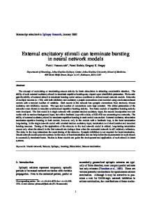
2. Model architectures 2.1. Feed forward neural network language model The architecture of a feed-forward NNLM is shown in Figure 1. The inputs to the neural network are indices of the previous n– 1 words, encoded using 1 of N (one-hot) coding. The feature vectors of each of the previous n–1 words are projected to a P -dimension continuous space using an N ⇥ P weight matrix. Since we use a one-hot representation for the words, this sim-

1000000

w i −2

P (w i=1 /hi )

W

0000001

W

N

H

U w i −1

N

p

V

w3 P (w i= j /hi )

P (w i= N /h i)

Figure 1: Feed-forward neural network language model[2, 3]

H

f w1

f

0100000

w (t )

w1

000100

010000

w i −2

w i −1

0001000

sj (t) = f

U

H

V

N

yk (t) = g

Figure 2: Recurrent neural network language model[5]

plifies to copying the ith row of N ⇥ P matrix in the case of the ith word in the vocabulary. The same weight matrix is used to project other words in the context. The P -dimensional features of the context words are concatenated and provided as an input to the hidden layer, which typically uses a tanh activation function. In the output layer, a softmax function is used to compute the probability of a word given the context. The size of the softmax layer is the size of the vocabulary, N . The activations of projection and hidden layer, and the output probability distribution are computed as follows: X

uji fi + bj

i=1

ak =

H X

!

8j = 1, ......., H

(1)

vkj hj + bk

j=1

e ak yk = P N k=1

eak

8k = 1, ......, N .

(2)

In this work, we use a factored output layer [6] to reduce the computational complexity. 2.2. Recurrent neural network language models

X

xi (t)uji

(4)

sj (t)vkj

!

(5)

1)]

Where x(t) is the input vector, s(t) is the state of hidden layer at time t and y(t) is the output probability distribution. f , g are sigmoid activation and softmax functions, respectively. The objective of training is to maximize the likelihood of training data by minimizing the cross entropy difference between the target and output probability distributions, using BPTT. The number of steps for which the error is propagated back in time is optimized for minimum perplexity on a validation set. In all the experiments reported in this work, the error is propagated three steps back in time and a factored output layer is used to reduce the computational complexity. 2.3. Pre-trained Recurrent Neural Network Language Model (PT-RNNLM) In Figure 3, we show an architecture in which an RNNLM and a feed-forward NNLM are combined. The feed-forward and recurrent networks have the same number of hidden and output nodes, and the output layer weights of the two networks are shared. In the first phase of training, only the feed-forward weights are trained (using back-propagation). When the feedforward network has been trained for a number of iterations, the output layer weights are shared with the RNNLM, which may be interpreted as an initialisation or pre-training. During testing we only use the RNNLM part of PT-RNNLM to compute the probability distribution. Again, we used a factored output layer to reduce the computational requirement. We evaluated these models using text data (Wall Street Journal) and a perplexity measure, and using speech data (TED talks) and a word error rate (WER) measure.

3. Text experiments

The architecture of a RNN is shown in Figure 2. The input to the network at time t is the index of the previous word and the state of the hidden layer at time t–1. The index of the previous word is encoded using 1 of N coding. The hidden layer at time t and the output probability distribution are computed as follows: x(t) = [w(t), s(t

H s (t−1)

!

j

s (t−1)

hj = tanh

X i

H

(n 1)P

s (t) w4

Figure 3: Pre-trained recurrent neural network language model

y (t )

s (t)

H w2

p

w (t )

C

(3)

We report performed experiments on the Wall Street Journal (WSJ) data in the Penn Treebank (PTB)1 . Sections 0–20 were used as training data, sections 21–22 were used as validation data, and sections 23–24 used as test data. A 10,000 (10k) word vocabulary was used, with out of vocabulary words being mapped to a special token . The number of tokens 1 http://www.cis.upenn.edu/

treebank/

Model 3-gram NNLM RNNLM PT-RNNLM

Valid. PPL 162.4 173.4 155.5 150.7

+KN3 143.0 130.9 128.7

Test PPL 152.9 162.4 148.3 143.4

+KN3 135.1 124.9 123.0

Table 1: Perplexity of n-gram, NNLM, RNNLM and PTRNNLM trained on WSJ data. 100 hidden nodes and 100 output classes are used in NNLM, RNNLM and PT-RNNLM

4. Speech experiments 4.1. TED ASR task TED2 (Technology, Entertainment, Design) organises an international lecture series in wide range of disciplines. The lectures are transcribed (and translated) using crowdsourcing, thus providing about 200 hours of verbatim-transcribed data, which have been used for ASR and machine translation evaluation as part of the IWSLT evaluation campaign3 . In this work, we used the dev2010 and tst2010 sets for development and the tst2011 set for evaluation. The neural network language models are applied to the ASR system by re-scoring N-best lists (produced from a system using an n-gram language model). These scores may be interpolated with n-gram scores, with the interpolation coefficients being optimized on development data. 4.2. ASR system

Figure 4: The number of iterations of pre-training Vs perplexity of PT-RNNLM

in the training, validation and test sets were 930K, 74K and 82K words respectively. In each experiment reported in this section, 100 hidden nodes were used in NNLM, RNNLM and PTRNNLM. To reduce the computational complexity, a factored output layer is used in NNLM, RNNLM and PT-RNNLM. The dimension of the features in NNLM is 50. The baseline 3-gram is Kneser-Ney smoothed (KN3) with default count cut-offs. In the PT-RNNLM, first the weights of the NNLM were fine tuned, until the difference in entropy between iterations on a validation set was smaller than a predefined threshold. The weights of the RNNLM were then fine tuned, by initialising the output layer parameters with the fine tuned output layer parameters of NNLM. Perplexity (PPL) results are given in Table 1. We can observe 4.2% and 3.0% relative improvements in PPL for the RNNLM over the 3-gram baseline, on validation and test sets respectively. The PT-RNNLM further reduces PPL by 3.0% and 3.3% relative on the validation and test sets. There is a further 10–15% relative reduction in PPL (on both data sets) when the neural network models are interpolated with the KN3 baseline LMs. We investigated the behaviour of the PT-RNNLM with respect to the number of iterations of pre-training (Figure 4). There is a significant reduction in PPL after just one iteration of pre-training, and a slight downward trend for a further eight iterations, before the curve flattens. From this we can conclude a few iterations of pre-training is necessary to improve the prediction accuracy of RNNLM, and the feed-forward network does not need to be trained to completion.

The ASR system [18, 19] uses deep neural network-based acoustic models in both Tandem and Hybrid configurations, both of which use the Multi Level Adaptive Neural Network (MLAN) architecture for domain adaptation [18]. In the first step, deep neural networks were trained on out-of-domain (OOD). In the next step, the bottleneck features generated on in-domain data using DNNs trained on OOD data are concatenated with the in-domain features. These concatenated features are used to train Tandem and Hybrid MLAN HMMs. The training data consisted of 143 hours of transcribed and aligned TED lectures, and 127 hours of transcribed AMI4 meeting data used to train the OOD networks in MLAN. To avoid the overlap between development and evaluation sets all the selected lectures for training are dated before 2010. Tandem MLANs are trained with four hidden layers, each consists of 1024 hidden neurons. Six hidden layers are used in Hybrid MLANs, each layer consists of 2048 hidden neurons. All the scripts are written in Theano [20] and the models were trained on NVIDIA GeForce GTX 690 GPUs. 4.3. Language models 4.3.1. n-grams The ASR system uses Kneser-Ney (KN) smoothed n-gram language models for decoding and lattice rescoring. The n-gram language models are obtained by interpolating the language models trained on 2.4M in-domain and 312M OOD word tokens. Given the mismatch between in-domain and OOD data, the relevant sentences to the task domain are selected by computing the cross entropy difference (CED) score [21] for each sentence s: DS = {s|HI (s)

HO (s) < ⌧ }

(6)

where HI (s) is a cross-entropy of a sentence with a LM trained on in-domain data, HO (s) is a cross-entropy of a sentence with a LM trained on a random subset of the OOD data of similar size to the TED in-domain data, and ⌧ is a threshold to control the size of DS . The OOD data sources include Europarl, News Commentary, News Crawl, and Gigaword. In the final ASR system KN smoothed 3-gram and 4-gram LMs are used for decoding and lattice rescoring, respectively. 2 http://www.ted.com

3 http://www.iwslt2013.org

4 https://www.idiap.ch/dataset/ami

Model

PPL

4-gram RNNLM-7.4M PT-RNNLM-7.4M RNNLM-12.4M PT-RNNLM-12.4M RNNLM-22.4M PT-RNNLM-22.4M

124 161 159 145 144 132 129

Tandem MLAN HMM dev2010 tst2010 tst2011 15.47 13.50 10.57 15.04 13.13 10.30 14.94 13.03 10.22 14.85 12.78 10.10 14.75 12.72 10.13 14.71 12.59 10.06 14.46 12.57 9.86

Table 2: % WERs of n-gram, RNNLM and PT-RNNLM, trained on combination of in-domain and subsets of OOD data (Tandem acoustic model). 4.3.2. RNN language models Given the complexity of training RNNLM and PT-RNNLM on large amounts of data, we have trained the RNNLM and PTRNNLM on combination of in-domain and different subsets of OOD data, selected using CED metric, as described in Section 4.3.1. All the distinct words in the in-domain data are retained and the words with frequency 1 in the OOD data are replaced with label. The neural nets are trained until the difference in entropy between two successive iterations is less than a predefined threshold. In all the experiments reported in this work the threshold is 0.01. The validation data for early stopping – the combination of dev2010 and tst2010 – contains a total 44K tokens. 4.4. Results We report WER and PPL on the dev2010, tst2010 and tst2011 data sets. The RNNLM and PT-RNNLM are trained on combinations of in-domain data (2.4M word tokens) and three subsets of OOD data (5M, 10M and 20M tokens). The number of hidden neurons and number of classes in the output layer are optimized for better WER. The models trained on 7.4M tokens consists of 300 hidden neurons and the models trained on 12.4M and 22.4M tokens consists of 500 hidden neurons. In all the experiments reported here 100 classes are used in the output layer to reduce the computational complexity. All the models were trained on a computing cluster hosting Intel Xeon E5645 processors. Approximately, it takes 30 hours, 70 hours and one week to train the models on 7.4M, 12.4M, 22.4M tokens respectively. The WERs after rescoring the the 100-best lists of Tandem MLAN HMMs are given in Table 2. The PT-RNNLM reduces the WERs by 0.1% over the RNNLM, in second section of Table 2. The models trained on more OOD data in combination with the in-domain data further reduce the WERs. In third section of Table 2, the reductions in the WERs with the PT-RNNLM are in the range of 0.06%-0.1%. Surprisingly the WER of PT-RNNLM on tst2011 is slightly higher than RNNLM. Similarly, the models trained on 22.4M tokens further reduce the WERs, in fourth section of Table 2. If we compare all the reported results on development and test sets, the proposed PT-RNNLM reduces the WERs in most of the cases and the reductions are consistent across data sets. We also report the WER after rescoring the 100-best lists produced using Hybrid MLAN HMMs. In second section of Table 3, we can observe, the PT-RNNLM reduces WERs of dev2010 by 0.1%, tst2011 by 0.25% and the WER of tst2010 is almost equal to that of RNNLM. As expected the models trained on more OOD data in combination with the in-domain data fur-

ther reduce the WERs. In section three and four of Table 3, we can observe the reductions in WERs are in the range of 0.1%0.23% and 0.1%-0.15%, respectively. To measure the statistical significance of a difference between two speech recognition algorithms, a paired test can be run on their respective error rates, measured per utterance or per segment so as to represent a set of independent samples [22]. In the present case, the appropriate granularity of measurement was judged to be at the level of results per TED talk, since the results within any one talk were on a fixed speaker and topic, and hence were not independent samples, but the speaker and topic changed between talks. Also it was the overall difference between RNNLM and PT-RNNLM that was of interest, rather than the difference on a specific training set size and with a specific acoustic model type. Therefore, a paired samples t-test (two-tailed) was run on the per-talk average word error rates with RNNLM and PT-RNNLM, where the averaging for each talk and language modelling technique was over the three training data sizes (7.4M, 12.4M and 22.4M words) and the tandem and hybrid models. This was done on the full set of 27 talks (8 in dev2010, 11 in tst2010 and 8 in tst2011). The result was a highly significant difference (p = 0.000275) in favour of PTRNNLM. This is significant at the 0.001 level, as recommended in a recent analysis of significance levels with regard to strength of evidence assessed by the corresponding Bayesian tests [23]. Model

PPL

4-gram RNNLM-7.4M PT-RNNLM-7.4M RNNLM-12.4M PT-RNNLM-12.4M RNNLM-22.4M PT-RNNLM-22.4M

124 161 159 145 144 132 129

Hybrid MLAN HMM dev2010 tst2010 tst2011 15.14 13.48 11.22 14.91 13.04 10.83 14.81 13.05 10.58 14.61 12.81 10.47 14.52 12.67 10.24 14.45 12.57 10.07 14.30 12.48 9.95

Table 3: % WERs of n-gram, RNNLM and PT-RNNLM, trained on combination of in-domain and subsets of OOD data (Hybrid acoustic model).

5. Conclusions and Future work In this work we have proposed feed forward pre-training for RNNLM by sharing the output weights of NNLM with the RNNLM. We report perplexity results on WSJ/PTB data, with the PT-RNNLM reducing perplexity on both the validation and test sets. We also investigated how many iterations of feed forward pre-training is necessary to improve the prediction accuracy of RNNLM. We have observed a few iterations of pretraining is sufficient. Finally we report the WERs on by rescoring 100-best lists of Tandem and Hybrid MLAN HMMs for the IWSLT TED talk recognition task, and observed a small but significant reduction in WER from the PT-RNNLM over the RNNLM. There are a number of further approaches which we are investigating to combine feed-forward and recurrent NNLMs. This includes co-training rather than pre-training (i.e. training the output weights is interleaved between the feed-forward and recurrent neural networks), sharing the projected continuous space representations between the two architectures and combining the feed-forward and recurrent architectures without output weight sharing.

6. References [1] F. Jelinek, Statistical Methods for Speech Recognition. Press, 1998.

MIT

[2] Y. Bengio, R. Ducharme, P. Vincent, and C. Jauvin, “A neural probabilistic language model,” Journal of Machine Learning Research, vol. 3, pp. 1137–1155, 2003. [3] H. Schwenk, “Continuous space language models,” Computer Speech & Language, vol. 21, no. 3, pp. 492–518, 2007. [4] J. Park, X. Liu, M. J. F. Gales, and P. C. Woodland, “Improved neural network based language modelling and adaptation,” in Proc Interspeech, 2010, pp. 1041–1044. [5] T. Mikolov, M. Karafi´at, L. Burget, J. Cernock´y, and S. Khudanpur, “Recurrent neural network based language model,” in Proc Interspeech, 2010, pp. 1045–1048. [6] T. Mikolov, S. Kombrink, L. Burget, J. Cernock´y, and S. Khudanpur, “Extensions of recurrent neural network language model,” in Proc IEEE ICASSP, 2011, pp. 5528–5531. [7] P. J. Werbos, “Backpropagation through time: what it does and how to do it,” Proceedings of the IEEE, vol. 78, no. 10, pp. 1550– 1560, 1990. [8] S. Hochreiter, “Untersuchungen zu dynamischen neuronalen netzen,” Diploma thesis, Institut f¨ur Informatik, Technische Universit¨at M¨unchen, 1991. [9] Y. Bengio, P. Simard, and P. Frasconi, “Learning long-term dependencies with gradient descent is difficult,” IEEE Trans. Neural Networks, vol. 5, no. 2, pp. 157–166, 1994. [10] T. Robinson and F. Fallside, “A recurrent error propagation network speech recognition system,” Computer Speech and Language, vol. 5, pp. 259–274, 1991. [11] T. Robinson, M. Hochberg, and S. Renals, “The use of recurrent networks in continuous speech recognition,” in Automatic Speech and Speaker Recognition – Advanced Topics, C. H. Lee, K. K. Paliwal, and F. K. Soong, Eds. Kluwer Academic Publishers, 1996, ch. 10, pp. 233–258. [12] A. J. Robinson, G. D. Cook, D. P. W. Ellis, E. Fosler-Lussier, S. J. Renals, and D. A. G. Williams, “Connectionist speech recognition of broadcast news,” Speech Communication, vol. 37, no. 1–2, pp. 27–45, 2002. [13] R. Williams and D. Zipser, “A learning algorithm for continually running fully recurrent neural networks,” Neural Computation, vol. 1, no. 2, pp. 270–280, 1989. [14] U. Naumann, The Art of Differentiating Computer Programs: An Introduction to Algorithmic Differentiation. SIAM, 2012. [15] I. Sutskever, J. Martens, G. Dahl, and G. Hinton, “On the importance of initialization and momentum in deep learning,” in Proc ICML, 2013. [16] E. Hasler, P. Bell, A. Ghoshal, B. Haddow, P. Koehn, F. McInnes, S. Renals, and P. Swietojanski, “The UEDIN system for the IWSLT 2012 evaluation,” in Proc. International Workshop on Spoken Language Translation, 2012. [17] P. Bell, F. McInnes, S. Gangireddy, M. Sinclair, A. Birch, and S. Renals, “The UEDIN English ASR system for the IWSLT 2013 evaluation,” in Proc. International Workshop on Spoken Language Translation, 2013. [18] P. Bell, P. Swietojanski, and S. Renals, “Multi-level adaptive networks in tandem and hybrid ASR systems,” in ICASSP. IEEE, 2013, pp. 6975–6979. [19] P. Bell, H. Yamamoto, P. Swietojanski, Y. Wu, F. McInnes, C. Hori, and S. Renals, “A lecture transcription system combining neural network acoustic and language models,” in Proc Inbterspeech, 2013, pp. 3087–3091. [20] J. Bergstra, O. Breuleux, F. Bastien, P. Lamblin, R. Pascanu, G. Desjardins, J. Turian, D. Warde-Farley, and Y. Bengio, “Theano: a CPU and GPU math expression compiler,” in Proceedings of the Python for Scientific Computing Conference (SciPy), 2010.

[21] R. C. Moore and W. D. Lewis, “Intelligent selection of language model training data,” in ACL (Short Papers), 2010, pp. 220–224. [22] L. Gillick and S. Cox, “Some statistical issues in the comparison of speech recognition algorithms,” in Proc. ICASSP, 1989, pp. 532–535. [23] V. E. Johnson, “Revised standards for statistical evidence,” Proc. National Academy of Sciences of the USA, vol. 110, no. 48, pp. 19 313–19 317, 2013.