Multimodal Neural Language Models
Ryan Kiros Ruslan Salakhutdinov Richard Zemel Department of Computer Science, University of Toronto Canadian Institute for Advanced Research
Abstract We introduce two multimodal neural language models: models of natural language that can be conditioned on other modalities. An imagetext multimodal neural language model can be used to retrieve images given complex sentence queries, retrieve phrase descriptions given image queries, as well as generate text conditioned on images. We show that in the case of image-text modelling we can jointly learn word representations and image features by training our models together with a convolutional network. Unlike many of the existing methods, our approach can generate sentence descriptions for images without the use of templates, structured prediction, and/or syntactic trees. While we focus on imagetext modelling, our algorithms can be easily applied to other modalities such as audio.
RKIROS @ CS . TORONTO . EDU RSALAKHU @ CS . TORONTO . EDU ZEMEL @ CS . TORONTO . EDU
In this paper we introduce multimodal neural language models, models of natural language that can be conditioned on other modalities. A multimodal neural language model represents a first step towards tackling the previously described modelling challenges. Unlike most previous approaches to generating image descriptions, our model makes no use of templates, structured models, or syntactic trees. Instead, it relies on word representations learned from millions of words and conditioning the model on high-level image features learned from deep neural networks. We introduce two methods based on the log-bilinear model of Mnih & Hinton (2007): the modality-biased logbilinear model and the factored 3-way log-bilinear model. We then show how to learn word representations and image features together by jointly training our language models with a convolutional network. Experimentation is performed on three datasets with image-text descriptions: IAPR TC-12, Attributes Discovery, and the SBU datasets. We further illustrate capabilities of our models through quantitative retrieval evaluation and visualizations of our results.
1. Introduction Descriptive language is almost never isolated from other modalities. Advertisements come with images of the product that is being sold, social media profiles contain both descriptions and images of the user while multimedia websites that play audio and video have associated descriptions and opinions of the content. Consider the task of creating an advertisement to sell an item. An algorithm that can model both text descriptions and pictures of the item would allow a user to (a): search for pictures given a text description of the desired content; (b): find similar item descriptions given uploaded images; and (c): automatically generate text to describe the item given pictures. What these tasks have in common is the need to go beyond simple bagof-word representations of text alone to model complex descriptions with an associated modality. Proceedings of the 31 st International Conference on Machine Learning, Beijing, China, 2014. JMLR: W&CP volume 32. Copyright 2014 by the author(s).
2. Related Work Our related work can largely be separated into three groups: neural language models, image content description and multimodal representation learning. Neural Language Models: A neural language model improves on n-gram language models by reducing the curse of dimensionality through the use of distributed word representations. Each word in the vocabulary is represented as a real-valued feature vector such that the cosine of the angles between these vectors is high for semantically similar words. Several models have been proposed based on feedforward networks (Bengio et al., 2003), log-bilinear models (Mnih & Hinton, 2007), skip-gram models (Mikolov et al., 2013) and recurrent neural networks (Mikolov et al., 2010; 2011). Training can be sped up through the use of hierarchical softmax (Morin & Bengio, 2005) or noise contrastive estimation (Mnih & Teh, 2012).
Multimodal Neural Language Models
Figure 1. Left two columns: Sample description retrieval given images. Right two columns: description generation. Each description was initialized to ‘in this picture there is’ or ‘this product contains a’, with 50 subsequent words generated.
Image Description Generation: A growing body of research has explored how to generate realistic text descriptions given an image. Farhadi et al. (2010) consider learning an intermediate meaning space to project image and sentence features allowing them to retrieve text from images and vice versa. Kulkarni et al. (2011) construct a CRF using unary potentials from objects, attributes and prepositions and high-order potentials from text corpora, using an n-gram model for decoding and templates for constraints. To allow for more descriptive and poetic generation, Mitchell et al. (2012) propose the use of syntactic trees constructed from 700,000 Flickr images and text descriptions. For large scale description generation, Ordonez et al. (2011) showed that non-parametric approaches are effective on a dataset of one million image-text captions. More recently, Socher et al. (2014) show how to map sentence representations from recursive networks into the same space as images. We note that unlike most existing work, our generated text comes directly from language model samples without any additional templates, structure, or constraints.
duced the multimodal deep Boltzmann machine as a joint model of images and text. Unlike Srivastava & Salakhutdinov (2012), our proposed models are conditional and go beyond bag-of-word features. More recently, Socher et al. (2013) and Frome et al. (2013) propose methods for mapping images into a text representation space learned from a language model that incorporates global context (Huang et al., 2012) or a skip-gram model (Mikolov et al., 2013), respectively . This allowed Socher et al. (2013); Frome et al. (2013) to perform zero-shot learning, generalizing to classes the model has never seen before. Similar to our work, the authors combine convolutional networks with a language model but our work instead focuses on text generation and retrieval as opposed to object classification.
Multimodal Representation Learning: Deep learning methods have been successfully used to learn representations from multiple modalities. Ngiam et al. (2011) proposed using deep autoencoders to learn features from audio and video, while Srivastava & Salakhutdinov (2012) intro-
3. The Log-Bilinear Model (LBL)
The remainder of the paper is structured as follows. We first review the log-bilinear model of Mnih & Hinton (2007) as it forms the foundation for our work. We then introduce our two proposed models as well as how to perform joint image-text feature learning. Finally, we describe our experiments and results.
The log-bilinear language model (LBL) (Mnih & Hinton, 2007) is a deterministic model that may be viewed as a feed-forward neural network with a single linear hidden
Multimodal Neural Language Models
layer. As a neural language model, the LBL operates on word representation vectors. Each word w in the vocabulary is represented as a D-dimensional real-valued vector rw ∈ RD . Let R denote the K × D matrix of word representation vectors where K is the vocabulary size. Let (w1 , . . . wn−1 ) be a tuple of n − 1 words where n − 1 is the context size. The LBL model makes a linear prediction of the next word representation as ˆ r=
n−1 X
(i)
C rwi ,
(1)
i=1
where C(i) , i = 1, . . . , n − 1 are D × D context parameter matrices. Thus, ˆ r is the predicted representation of rwn . The conditional probability P (wn = i|w1:n−1 ) of wn given w1 , . . . , wn−1 is exp(ˆ rT ri + bi ) , P (wn = i|w1:n−1 ) = PK rT rj + bj ) j=1 exp(ˆ
(2)
where b ∈ RK is a bias vector with a word-specific bias bi . Eq. 2 may be seen as scoring the predicted representation ˆ r of wn against the actual representation rwn through an inner product, followed by normalization based on the inner products amongst all other word representations in the vocabulary. In the context of a feed-forward neural network, the weights between the output layer and linear hidden layer is the word representation matrix R where the output layer uses a softmax activation. Learning can be done with standard backpropagation.
4. Multimodal Log-Bilinear Models Suppose that along with each training tuple of words (w1 , . . . wn ) there is an associated vector x ∈ RM corresponding to the feature representation of the modality to be conditioned on, such as an image. Assume for now that these features are computed in advance. In Section 5 we show how to jointly learn both text and image features. 4.1. Modality-Biased Log-Bilinear Model (MLBL-B) Our first proposed model is the modality-biased logbilinear model (MLBL-B) which is a straightforward extension of the LBL model. The MLBL-B model adds an additive bias to the next predicted word representation ˆ r which is computed as ! n−1 X (i) ˆ r= C rwi + C(m) x, (3) i=1
where C(m) is a D × M context matrix. Given the predicted next word representation ˆ r, computing the conditional probability P (wn = i|w1:n−1 , x) of wn given w1 , . . . , wn−1 and x remains unchanged from the LBL
model. The MLBL-B can be viewed as a feedforward network by taking the LBL network and adding a context channel based on the modality x, as shown in Fig. 2a. This model also shares resemblance to the quadratic model of Grangier et al. (2006). Learning in this model involves a straightforward application of backpropagation as in the LBL model. 4.2. The Factored 3-way Log-Bilinear Model (MLBL-F) A more powerful model to incorporate modality conditioning is to gate the word representation matrix R by the features x. By doing this, R becomes a tensor for which each feature x can specify its own hidden to output weight matrix. More specifically, let R(1) , . . . , R(m) be K × D matrices specified by feature components 1, . . . , M of x. The hidden to output weights corresponding to x are computed as M X Rx = xi R(i) , (4) i=1 x
where R denotes the word representations with respect to x. The motivation for using a modality specific word representation is as follows. Suppose x is an image containing a picture of a cat, with context words (there, is, a). A language model that is trained without knowledge of image features would score the predicted next word representation ˆ r high with words such as dog, building or car. If each image has a corresponding word representation matrix Rx , the representations for attributes that are not present in the image would be modified such that the inner product of ˆ r with the representation of cat would score higher than the inner product of ˆ r with the representations of dog, building or car. As is, the tensor R requires K × D × M parameters which makes using a general 3-way tensor impractical even for modest vocabulary sizes. A common solution to this approach (Memisevic & Hinton, 2007; Krizhevsky et al., 2010) is to factor R into three lower-rank matrices Wf rˆ ∈ RF ×D , Wf x ∈ RF ×M and Wf h ∈ RF ×K , such that Rx = (Wf h )> · diag(Wf x x) · Wf rˆ,
(5)
where diag(·) denotes the matrix with its argument on the diagonal. These matrices are parametrized by F , the number of factors, as shown in Fig. 2b. Let E = (Wf rˆ)> Wf h denote the D × K matrix of word embeddings. Given the context w1 , . . . , wn−1 , the predicted next word representation ˆ r is given by: ! n−1 X (i) ˆ r= C E(:, wi ) + C(m) x, (6) i=1
where E(:, wi ) denotes the column of E for the word representation of wi . Given a predicted next word representation
Multimodal Neural Language Models
steam
steam rw 1
ship
C2
rw 2
in
rw 3
rw 1
C1 ˆ r
R
h
C3
aardvark abacus ... zebra
Cm
(a) Modality-Biased Log-Bilinear Model (MLBL-B)
ship
C2
C1
rw 2
in
rw 3
ˆ r C3
Wf rˆ
Wf h Wf x
h
aardvark abacus ... zebra
Cm
(b) Factored 3-way Log-Bilinear Model (MLBL-F)
Figure 2. Our proposed models. Left: The predicted next word representation ˆ r is a linear prediction of word features rw1 , rw2 , rw3 (blue connections) biased by image features x. Right: The word representation matrix R is replaced by a factored tensor for which the hidden-to-output connections are gated by x.
ˆ r, the factor outputs are f = (Wf rˆˆ r) • (Wf x x),
(7)
where • is a component-wise product. The conditional probability P (wn = i|w1:n−1 , x) of wn given w1 , . . . , wn−1 and x can be written as � exp (Wf h (:, i))> f + bi P (wn = i|w1:n−1 , x) = PK �, fh > j=1 exp (W (:, j)) f + bj where Wf h (:, i) denotes the column of Wf h corresponding to word i. We call this the MLBL-F model. As with the LBL and MLBL-B models, training can be achieved using a straightforward application of backpropagation. Unlike the other models, extra care needs to be taken when adjusting the learning rates for the matrices of the factored tensor. It is sensible that pre-computed word embeddings could be used as a starting point to training, as opposed to random initialization of the word representations. Indeed, all of our experiments use the embeddings of Turian et al. (2010) for initialization. In the case of the LBL and MLBL-B models, each pre-trained word embedding can be used to initialize the rows of R. In the case of the MLBL-F model where R is a factored tensor, we can let E be the D × K matrix of pre-trained embeddings. Since E = (Wf rˆ)> Wf h , we can initialize the MLBL-F model with pre-trained embeddings by simply applying an SVD to E.
5. Joint Image-Text Feature Learning Up until now we have not made any assumptions on the type of modality being used for the feature representation x. In this section, we consider the case where the conditioned modality consists of images and show how to jointly learn image and word features along with the model parameters. One way of incorporating image representation learning is to use a convolutional network for which the outputs are
used either as an additive bias or for gating. Gradients from the loss could then be backpropagated from the language model through the convolutional network to update filter weights. Unfortunately, learning on every image in this architecture is computationally demanding. Since each training tuple of words comes with an associated image, then the number of training elements becomes large even with a modest size training set. For example, if the training set consisted of 10,000 images and each image had a text description of 20 words, then the number of training elements for the model becomes 200,000. For large image databases this could quickly scale to millions of training instances. To speed up computation, we follow Wang et al. (2012); Swersky et al. (2013) and learn our convolutional networks on small feature maps learned using k-means as opposed to the original images. We follow the pipeline of Coates & Ng (2011). Given training images, r × r patches are randomly extracted, contrast normalized and whitened. These are used for training a dictionary with spherical k-means. These filters are convolved with the image and a soft activation encoding is applied. If the image is of dimensions nV ×nH ×3 and kf filters are learned, the resulting feature maps are of size (nV − r + 1) × (nH − r + 1) × kf . Each slice of this region is then split into a G × G grid for which features within each region are max-pooled. This results in an output of size G × G × kf . It is these outputs that are used as inputs to the convolutional network. For all of our experiments, we use G = 9 and kf = 128. Each 9 × 9 × 128 input is convolved with 64 3 × 3 filters resulting in feature maps of size 7 × 7 × 64. Rectified linear units (ReLUs) are used for activation followed by a response normalization layer (Krizhevsky et al., 2012). The response-normalized feature maps are then max-pooled with a pooling window of 3 × 3 and a stride of 2, resulting in outputs of size 3 × 3 × 64. One fully-connected layer with ReLU activation is added. It is the feature responses at this layer that are used either for additive biasing or gating in the MLBL-B and MLBL-F models, respectively.
Multimodal Neural Language Models
6. Generation and Retrieval
7. Experiments
The standard approach to evaluating language models is through perplexity
We perform experimental evaluation of our proposed models on three publicly available datasets:
log2 C(w1:n |x) = −
1 X log2 P (wn = i|w1:n−1 , x), Nw 1:n
where w1:n−1 runs through each subsequence of length n − 1 and N is the length of the sequence. Here we use perplexity not only as a measure of performance but also as a link between text and the additional modality. First, consider the task of retrieving training images from a text query w1:N . For each image x in the training set, we compute C(w1:N |x) and return the images for which C(w1:N |x) is lowest. Intuitively, images when conditioned on by the model that achieve low perplexity are those that are a good match to the query description. The task of retrieving text from an image query is trickier for the following reasons. It is likely that there are many ‘easy’ sentences for which the language model will assign low perplexity to independent of the query image being conditioned on. Thus, instead of retrieving text from the training set for which C(w1:N |x) is lowest conditioned on the query image x, we instead look at the ratio C(w1:N |x)/C(w1:N |˜ x) where x ˜ denotes the mean image in the training set (computed in feature space). Thus, if w1:N is a good explanation of x, then C(w1:N |x) < C(w1:N |˜ x) and we can simply retrieve the text for which this ratio is smallest. While this leads to better search results, it is conceivable that using the image itself as a query for other images and returning their corresponding descriptions may in itself work well as a query strategy. For example, an image taken at night would ideally return a description describing this, which would be more likely to occur if we first retrieved nearby images which were also taken at night. We found the most effective way of performing description retrieval is as follows: first retrieve the top kr training images as a shortlist based on the Euclidean distance between x and images in the training set. Then retrieve the descriptions for which C(w1:N |x)/C(w1:N |˜ x) is smallest for each description w1:N in the shortlist. We found that combining these two strategies is more effective than using either alone. In the case when a convolutional network is used, we first map the images through the convolutional network and use the output representations for computing distances. Finally, we generate text given an image as follows: Suppose we are given an initialization w1:n−1 , where n − 1 is the context size. We compute P (wn = i|w1:n−1 , x) and obtain a sample w ˜ from this distribution, appending w ˜ to our initialization. This procedure is then repeated for as long as desired.
IAPR TC-12 This data set consists of 20,000 images across various domains, such as landscapes, portraits, indoor and sports scenes. Accompanying each image is a text description of one to three sentences describing the content of the image. The dataset was initially released for crosslingual retrieval (Grubinger et al., 2006) but has since been used extensively for other tasks such as image annotation. We used a publicly available train/test split for our experiments. Attribute Discovery This dataset contains roughly 40,000 images related to products such as bags, clothing and shoes as well as subcategories of each product, such as highheels and sneakers. Each image is accompanied by a webretrieved text description which often reads as an advertisement for the product. Unlike the IAPR dataset, the text descriptions are not guaranteed to be descriptive of the image and often contain noisy, unrelated text. This dataset was proposed as a means of discovering visual attributes from noisy text (Berg et al., 2010). We used a random train/test split for our experiments which will be made publicly available. SBU Captioned Photos We obtained a subset of roughly 400,000 images from the SBU dataset (Ordonez et al., 2011) which contain images and short text descriptions. This dataset is used to induce word embeddings learned from both images and text for qualitative comparison. 7.1. Details of Experiments We perform four experiments, three of which are quantitative and one of which is qualitative: Bleu Evaluation Our main evaluation criteria is based on Bleu (Papineni et al., 2002). Bleu was designed for automated evaluation of statistical machine translation and can be used in our setting to measure similarity of descriptions. Previous work on generating text descriptions for images use Bleu as a means of evaluation, where the generated sentence is used as a candidate for the gold standard reference generation. Given the diversity of possible image descriptions, Bleu may penalize candidates which are arguably descriptive of image content as noted by Kulkarni et al. (2011) and may not always be the most effective evaluation (Hodosh et al., 2013), though Bleu remains the standard evaluation criteria for such models. Given a model, we generate a candidate description as described in Section 6, generating as many words as there are in the reference sentence and compute the Bleu score of the candidate with the reference. This is repeated over all test points ten times, in order to account for the variability in the generated sentences. For baselines, we also compare against the
Multimodal Neural Language Models Table 1. Sample neighbors (by cosine similarity) of words learned from the SBU dataset. First row: neighbors from Collobert & Weston (2008) (C&W). Second row: neighbors from a LBL model (without images). Third row: neighbors from a MLBL-F model (with images). gloomy classroom flower lighthouse cup terrain
tranquil dismal hazy laptop pub library bamboo bird plant breakwater monument pier championship cider bag shorelines seas headland
sensuous slower stormy dorm cabin desk silk tiger flowers icefield lagoon ship trophy bottle bottle topography paces chasm
somber feeble foggy desk library restroom gold monster fruit lagoon kingdom dock bowl needle container vegetation descent creekbed
log-bilinear model was well as image-conditioned models conditioned on random images. This allows us to obtain further evidence of the relevance of generated text. Finally, we compare against the models of Gupta et al. (2012) and Gupta & Mannem (2012) who report Bleu scores for their models on the IAPR dataset.1 Perplexity Evaluation Each of our proposed models are trained on both datasets and the perplexity of the language models are evaluated. As baselines, we also include the basic log-bilinear model as well as two n-gram models. To evaluate the effectiveness of using pre-trained word embeddings, we also train a log-bilinear model where the word representations are randomly initialized. We hypothesize that image-conditioned models should result in lower perplexity than models which are only trained on text without knowledge of their associated images. Retrieval Evaluation We quantitatively evaluate the performance of our model for doing retrieval. First consider the task of retrieving images from sentence queries. Given a test sentence, we compute the model perplexity conditioned on each test image and rank each image accordingly. Let kr denote the number of retrieved images. We define a sentence to be correctly matched if the matching image to the sentence query is ranked in the top kr images sorted by model perplexity. Retrieving sentences from image queries is performed equivalently. Since our models use a shortlist (see Section 6) of nearest images for retrieving sentences, we restrict our search to images within the shortlist, for 1
We note that an exact comparison cannot be made with these methods since Gupta & Mannem (2012) assume tags are given as input along with images and both methods apply 10-fold CV. The use of tags can substantially boost the relevance of generated sentences. Nonetheless, these methods provide context for our results.
bleak realistic crisp computer bedroom office bark cow green nunnery mosque castle league box oil convection yards ranges
cheerful brighter cloudless canteen office cabinet flesh fish plants waterway skyline marina tournament fashion net canyons rays crest
dreary strong dull darkroom cottage kitchen crab leaf rose walkway truck pool cups shoe jam slopes floors pamagirri
which the matching sentence is guaranteed to be in. For additional comparison, we include a strong imagebased bag-of-words baseline to determine whether a language model (and word ordering) is necessary for imagedescription retrieval tasks. This model works as follows: given image features, we learn a linear transformation onto independent logistic units, one for each P word in the description. Descriptions are scored as − N1 w1:n logP (wn = w|x). For retrieving images, we project each image and rank those which result in the highest description score. For retrieving sentences, we return those which result in the highest score given the word probabilities computed from the image. Since we use a shortlist for our models when performing sentence retrieval, we also use the same shortlist (relative to the image features used) to allow for fair comparison. A validation batch was used to tune the weight decay. Qualitative Results We trained a LBL model and a MLBL-F model on the SBU examples. Both language models were trained on the same text, but the MLBL-F also conditioned on images using DeCAF features (Donahue et al., 2013). Both models were trained using perplexity as a criteria for early stopping, and with the same context size and vocabulary. Table 1 shows sample nearest neighbors from both models. When trained on images and text, the MLBL-F model can learn to capture both visual and semantic similarities, resulting in very different nearest neighbors than the LBL model and C&W embeddings. These word embeddings will be made publicly available. We use three types of image features in our experiments: Gist (Oliva & Torralba, 2001), DeCAF (Donahue et al., 2013), and features learned jointly with a convolutional net.
Multimodal Neural Language Models Table 2. Results on IAPR TC-12. PPL refers to perplexity while B-n indicates Bleu scored with n-grams. Back-off GTn refers to n-grams with Katz backoff and Good-Turing discounting. Models which use a convolutional network are indicated by -conv, while -conv-R indicates using random images for conditioning. skmeans refers to the features of Kiros & Szepesv´ari (2012). M ODEL TYPE
PPL.
B-1
B-2
B-3
BACK - OFF GT2 BACK - OFF GT3 LBL MLBL-B- CONV- R MLBL-B- SKMEANS MLBL-F- SKMEANS MLBL-B-G IST MLBL-F-G IST MLBL-B- CONV MLBL-F- CONV MLBL-B-D E CAF MLBL-F-D E CAF G UPTA ET AL . G UPTA & M ANNEM
54.5 55.6 20.1 28.7 18.0 20.3 20.8 28.8 20.6 21.7 24.7 21.8 -
0.323 0.312 0.327 0.325 0.349 0.348 0.348 0.341 0.349 0.341 0.373 0.361 0.15 0.33
0.145 0.131 0.144 0.143 0.161 0.165 0.164 0.151 0.165 0.156 0.187 0.176 0.06 0.18
0.059 0.059 0.068 0.069 0.079 0.085 0.083 0.074 0.085 0.073 0.098 0.092 0.01 0.07
7.2. Details of Training Each of our language models were trained using the following hyperparameters: all context matrices used a weight decay of 1.0×10⁻⁴ while word representations used a weight decay of 1.0 × 10⁻⁵ . All other weight matrices, including the convolutional network filters use a weight decay of 1.0 × 10⁻⁴ . We used batch sizes of 20 and an initial learning rate of 0.2 (averaged over the minibatch) which was exponentially decreased at each epoch by a factor of 0.998. Gated methods used an initial learning rate of 0.02. Initial momentum was set to 0.5 and was increased linearly to 0.9 over 20 epochs. The word representation matrices were initialized to the 50 dimensional pre-trained embeddings of Turian et al. (2010). We used a context size of 5 for each of our models. Perplexity was computed starting with word C + 1 for all methods where C is the largest context size used in comparison (5 in our experiments). Perplexity was not evaluated on descriptions shorter than C + 3 words for all models. Since features used have varying dimensionality, an additional layer was added to map images to 256 dimensions, so that across all experiments the input size to the bias and gating units are equivalent. Note that we did not explore varying the word embedding dimensionalities, context sizes or number of factors. For each of our experiments, we split the training set into 80% training and 20% validation. Each model was trained while monitoring the perplexity on the validation set. Once the perplexity no longer improved for 5 epochs, the objective value on the training set was recorded. The training and validation sets were then fused and training continued until the objective value on the validation batch matched the recorded training objective. At this point, training stopped
Table 3. Results on the Attributes Discovery dataset. M ODEL TYPE
PPL.
B-1
B-2
B-3
BACK - OFF GT2 BACK - OFF GT3 LBL MLBL-B- CONV- R MLBL-B-G IST MLBL-F-G IST MLBL-B- CONV MLBL-F- CONV MLBL-B-D E CAF MLBL-F-D E CAF
117.7 93.4 97.6 154.4 95.7 115.1 99.2 113.2 98.3 133.0
0.163 0.166 0.161 0.166 0.185 0.182 0.189 0.175 0.186 0.178
0.033 0.032 0.031 0.035 0.044 0.042 0.048 0.042 0.045 0.041
0.009 0.011 0.009 0.012 0.013 0.013 0.017 0.014 0.014 0.012
and evaluation was performed on the test set. 7.3. Generation and Perplexity Results Tables 2 and 3 show results on the IAPR and Attributes dataset, respectively. On both datasets, each of our multimodal models outperforms both the log-bilinear and ngram models on Bleu scores. Our multimodal models also outperform Gupta et al. (2012) and result in comparable performance to Gupta & Mannem (2012). It should be noted that Gupta & Mannem (2012) assumes that both images and tags are given as input, where the presence of tags give substantial information about general image content. What is perhaps most surprising is that simple language models independent of images can also achieve nontrivial Bleu scores. For further comparison, we computed Bleu scores on the convolutional MLBL-B model when random images are used for conditioning. Moreover, we also computed Bleu scores on IAPR with LBL and MLBLB-DeCAF when stopwords are removed, obtaining (0.166, 0.052, 0.013) and (0.224, 0.082, 0.028) respectively. This gives us strong evidence that the gains in Bleu scores are obtained directly from capturing and associating word representations from image content. One observation from our results is that perplexity does not appear to be correlated with Bleu scores.2 On the IAPR dataset, the best perplexity is obtained using the MLBL-B model with fixed features, even though the best Bleu scores are obtained with a convolutional model. Similarly, both Back-off GT3 and LBL have the lowest perplexities on the Attributes dataset but are worse with respect to Bleu. Using more than 3-grams did not improve results on either dataset. For additional comparison, we also ran an experiment training LBL on both datasets using random word initialization, achieving perplexity scores of 23.4 and 109.6. This indicates the benefit of initialization from pre-trained word representations. Perhaps unsurprisingly, perplexity 2
This is likely due to high variance on held-out perplexities due to the shortness of text. We note that perplexity is lower on the training set with multimodal models.
Multimodal Neural Language Models Table 4. F-scores for retrieval on IAPR TC-12 when a text query is used to retrieve images (T → I) or when an image query is used to retrieve text (I → T ). Each row corresponds to DeCAF, Conv and Gist features, respectively.
T →I
Table 5. F-scores for retrieval on Attributes Discovery when a text query is used to retrieve images (T → I) or when an image query is used to retrieve text (I → T ). Each row corresponds to DeCAF, Conv and Gist features, respectively.
I→T
T →I
I→T
BOW
MLBL - B
MLBL - F
BOW
MLBL - B
MLBL - F
BOW
MLBL - B
MLBL - F
BOW
MLBL - B
MLBL - F
0.890 0.726 0.832
0.889 0.788 0.799
0.899 0.851 0.792
0.755 0.687 0.599
0.731 0.719 0.675
0.568 0.736 0.612
0.808 0.730 0.826
0.852 0.839 0.844
0.835 0.815 0.818
0.579 0.607 0.555
0.580 0.590 0.621
0.504 0.576 0.579
is much worse on the convolutional MLBL-B model when random images are used for conditioning.
included on the web page of the first author.
8. Conclusion 7.4. Retrieval Results Tables 4 and 5 illustrate the results of our retrieval experiments. In the majority of our experiments either the multimodal models outperform or are competitive with the bag-of-words baseline. The baseline when combined with DeCAF features is exceptionally strong. Perhaps this is unsurprising, given that these features were trained to predict object classes on ImageNet. The generality of these features also make it effective for predicting word occurrences, particularly if they are visual. For non-DeCAF experiments, our models improve on the baseline for 6 out of 8 tasks and result in near similar performance on another. The MLBL-F model performed best when combined with a convolutional net on IAPR while the MLBL-B model performed better on the remaining tasks. All 12 retrieval curves are included in the supplementary material. 7.5. Qualitative results The supplementary material contains qualitative results from our models. In general, the model does a good job at retrieving text with general characteristics of a scene or retrieving the correct type of product on the Attributes Discovery dataset, being able to distinguish between different kinds of sub-products, such as shoes and boots. The most common mistakes that the model makes are retrieving text with extraneous descriptions that do not exist in the image, such as describing people that are not present. We also observed errors on shorter queries where single words, such as sunset and lake, indicate key visual concepts that the model is not able to pick up on. For generating text, the model was initialized with ‘in this picture there is’ or ’this product contains a’ and proceeded to generate 50 words conditioned on the image. The model is often able to describe the general content of the image, even if it does not get specifics correct such as colors of clothing. This gives visual confirmation of the increased Bleu scores from our models. Several additional results are
In this paper we proposed multimodal neural language models. We described two novel language models and showed in the context of image-text learning how to jointly learn word representations and image features. Our models can obtain improved Bleu scores to existing approaches for sentence generation while generally outperforming a strong bag-of-words baseline for description and image retrieval. To our surprise, we found additive biasing with high-level image features to be quite effective. A key advantage of the multiplicative model though is speed of training: even with learning rates an order of magnitude smaller these models typically required substantially fewer epochs to achieve the same performance. Unlike MLBL-B, MLBL-F requires additional care in early stopping and learning rate selection. This work takes a first step towards generating image descriptions with a multimodal language model and sets a baseline when no additional structures are used. For future work, we intend to explore adding additional structures to improve syntax as well as combining our methods with a detection algorithm. ACKNOWLEDGMENTS We would also like to thank the anonymous reviewers for their valuable comments and suggestions. This work was supported by Google and ONR Grant N00014-14-1-0232.
References Bengio, Yoshua, Ducharme, R´ejean, Vincent, Pascal, and Janvin, Christian. A neural probabilistic language model. J. Mach. Learn. Res., 3:1137–1155, March 2003. Berg, Tamara L, Berg, Alexander C, and Shih, Jonathan. Automatic attribute discovery and characterization from noisy web data. In ECCV, pp. 663–676. Springer, 2010. Coates, Adam and Ng, Andrew. The importance of encoding versus training with sparse coding and vector quantization. In ICML, pp. 921–928, 2011.
Multimodal Neural Language Models Collobert, Ronan and Weston, Jason. A unified architecture for natural language processing: Deep neural networks with multitask learning. In ICML, pp. 160–167. ACM, 2008.
Mikolov, Tomas, Chen, Kai, Corrado, Greg, and Dean, Jeffrey. Efficient estimation of word representations in vector space. arXiv preprint arXiv:1301.3781, 2013.
Donahue, Jeff, Jia, Yangqing, Vinyals, Oriol, Hoffman, Judy, Zhang, Ning, Tzeng, Eric, and Darrell, Trevor. Decaf: A deep convolutional activation feature for generic visual recognition. arXiv preprint arXiv:1310.1531, 2013.
Mitchell, Margaret, Han, Xufeng, Dodge, Jesse, Mensch, Alyssa, Goyal, Amit, Berg, Alex, Yamaguchi, Kota, Berg, Tamara, Stratos, Karl, and Daum´e III, Hal. Midge: Generating image descriptions from computer vision detections. In EACL, pp. 747–756, 2012.
Farhadi, Ali, Hejrati, Mohsen, Sadeghi, Mohammad Amin, Young, Peter, Rashtchian, Cyrus, Hockenmaier, Julia, and Forsyth, David. Every picture tells a story: Generating sentences from images. In ECCV, pp. 15–29. Springer, 2010.
Mnih, Andriy and Hinton, Geoffrey. Three new graphical models for statistical language modelling. In ICML, pp. 641–648. ACM, 2007.
Frome, Andrea, Corrado, Greg S, Shlens, Jon, Bengio, Samy, Dean, Jeffrey, and MarcAurelio Ranzato, Tomas Mikolov. Devise: A deep visual-semantic embedding model. 2013.
Mnih, Andriy and Teh, Yee Whye. A fast and simple algorithm for training neural probabilistic language models. arXiv preprint arXiv:1206.6426, 2012.
Grangier, David, Monay, Florent, and Bengio, Samy. A discriminative approach for the retrieval of images from text queries. In Machine Learning: ECML 2006, pp. 162–173. Springer, 2006. Grubinger, Michael, Clough, Paul, M¨uller, Henning, and Deselaers, Thomas. The iapr tc-12 benchmark: A new evaluation resource for visual information systems. In International Workshop OntoImage, pp. 13–23, 2006. Gupta, Ankush and Mannem, Prashanth. From image annotation to image description. In NIP, pp. 196–204. Springer, 2012.
Morin, Frederic and Bengio, Yoshua. Hierarchical probabilistic neural network language model. In AISTATS, pp. 246–252, 2005. Ngiam, Jiquan, Khosla, Aditya, Kim, Mingyu, Nam, Juhan, Lee, Honglak, and Ng, Andrew. Multimodal deep learning. In ICML, pp. 689–696, 2011. Oliva, Aude and Torralba, Antonio. Modeling the shape of the scene: A holistic representation of the spatial envelope. IJCV, 42(3):145–175, 2001.
Gupta, Ankush, Verma, Yashaswi, and Jawahar, CV. Choosing linguistics over vision to describe images. In AAAI, 2012.
Ordonez, Vicente, Kulkarni, Girish, and Berg, Tamara L. Im2text: Describing images using 1 million captioned photographs. In NIPS, pp. 1143–1151, 2011.
Hodosh, Micah, Young, Peter, and Hockenmaier, Julia. Framing image description as a ranking task: data, models and evaluation metrics. JAIR, 47(1):853–899, 2013.
Papineni, Kishore, Roukos, Salim, Ward, Todd, and Zhu, WeiJing. Bleu: a method for automatic evaluation of machine translation. In ACL, pp. 311–318. ACL, 2002.
Huang, Eric H, Socher, Richard, Manning, Christopher D, and Ng, Andrew Y. Improving word representations via global context and multiple word prototypes. In ACL, pp. 873–882, 2012.
Socher, Richard, Ganjoo, Milind, Manning, Christopher D, and Ng, Andrew. Zero-shot learning through cross-modal transfer. In NIPS, pp. 935–943, 2013.
Kiros, Ryan and Szepesv´ari, Csaba. Deep representations and codes for image auto-annotation. In NIPS, pp. 917–925, 2012.
Socher, Richard, Le, Quoc V, Manning, Christopher D, and Ng, Andrew Y. Grounded compositional semantics for finding and describing images with sentences. TACL, 2014.
Krizhevsky, Alex, Hinton, Geoffrey E, et al. Factored 3-way restricted boltzmann machines for modeling natural images. In AISTATS, pp. 621–628, 2010.
Srivastava, Nitish and Salakhutdinov, Ruslan. Multimodal learning with deep boltzmann machines. In NIPS, pp. 2231–2239, 2012.
Krizhevsky, Alex, Sutskever, Ilya, and Hinton, Geoff. Imagenet classification with deep convolutional neural networks. In NIPS, pp. 1106–1114, 2012.
Swersky, Kevin, Snoek, Jasper, and Adams, Ryan. Multi-task bayesian optimization. In NIPS, 2013.
Kulkarni, Girish, Premraj, Visruth, Dhar, Sagnik, Li, Siming, Choi, Yejin, Berg, Alexander C, and Berg, Tamara L. Baby talk: Understanding and generating simple image descriptions. In CVPR, pp. 1601–1608. IEEE, 2011. Memisevic, Roland and Hinton, Geoffrey. Unsupervised learning of image transformations. In CVPR, pp. 1–8. IEEE, 2007. Mikolov, Tomas, Karafi´at, Martin, Burget, Lukas, Cernock`y, Jan, and Khudanpur, Sanjeev. Recurrent neural network based language model. In INTERSPEECH, pp. 1045–1048, 2010. Mikolov, Tomas, Deoras, Anoop, Povey, Daniel, Burget, Lukas, and Cernocky, Jan. Strategies for training large scale neural network language models. In ASRU, pp. 196–201. IEEE, 2011.
Turian, Joseph, Ratinov, Lev, and Bengio, Yoshua. Word representations: a simple and general method for semi-supervised learning. In ACL, pp. 384–394. Association for Computational Linguistics, 2010. Wang, Tao, Wu, David J, Coates, Adam, and Ng, Andrew Y. Endto-end text recognition with convolutional neural networks. In ICPR, pp. 3304–3308. IEEE, 2012.