Feature Extraction for Anomaly Detection in Maritime Trajectories

JOEL SUNDHOLM

Master’s Thesis at CSC Supervisor: Hedvig Kjellström Examiner: Danica Kragic Jensfelt Project Provider: Saab AB Supervisor at Project Provider: Rikard Laxhammar

Abstract The operators of a maritime surveillance system are hard pressed to make complete use of the near real-time information flow available today. To assist them in this matter there has been an increasing amount of interest in automated systems for the detection of anomalous trajectories. Specifically, it has been proposed that the framework of conformal anomaly detection can be used, as it provides the key property of a well-tuned alarm rate. However, in order to get an acceptable precision there is a need to carefully tailor the nonconformity measure used to determine if a trajectory is anomalous. This also applies to the features that are used by the measure. To contribute to a better understanding of what features are feasible and how the choice of feature space relates to the types of anomalies that can be found we have evaluated a number of features on real maritime trajectory data with simulated anomalies. It is found that none of the tested feature spaces was best for detecting all anomaly types in the test set. While one feature space might be best for detecting one kind of anomaly, another feature space might be better for other anomalies. There are indications that the best possible nonconformity measure should capture both absolute anomalies, such as an anomalous position, as well as relative anomalies, such as strange turns or stops.

Extrahering av egenskaper för anomalidetektion i maritima banor Referat För operatörerna av ett marint övervakningssystem är det en omöjlighet att göra en genomgripande analys av all realtidsdata som finns tillgänglig idag. För att assistera dem i deras arbete har det på senare tid utvecklats ett intresse för system som per automatik kan upptäcka anomaliska skeppsbanor. Specifikt har det föreslagits att ramverket conformal anomaly detection kan användas på grund av att det tillhandahåller en välkalibrerad larmfrekvens vilket är en nyckelegenskap för ett anomalidetektionssystem. För att åstadkomma en acceptabel precision finns det dock ett behov att omsorgsfullt skräddarsy den funktion, eller nonconformity measure, som används för att avgöra om en bana är anomalisk eller ej. Av vikt är också att skräddarsy de features som matas in i funktionen. För att bidra till en bättre förståelse för vilka features som är användbara och hur valet av dem påverkar vilka typer av anomalier vi kan upptäcka har en rad features utvärderats på riktig inspelad sjötrafiksdata med simulerade anomalier. Slutsatserna som kan dras från våra experiment är att ingen feature-rymd är bäst på att upptäcka alla sorters anomalier. Det finns indikationer på att den bästa möjliga feature-rymden bör kunna upptäcka både absoluta anomalier, så som en anomalisk position, såväl som relativa anomalier, det vill säga anomaliska rörelser.

Contents 1 Introduction 1.1 Contribution . . . . . . . . . . . . . . . . . . . . . . . . . . . . . . . 1.2 Outline . . . . . . . . . . . . . . . . . . . . . . . . . . . . . . . . . .

1 2 2

2 Background 2.1 Anomaly Detection . . . . . . . . . . . . . . . . . . . . . . . . . . . . 2.2 Conformal Prediction . . . . . . . . . . . . . . . . . . . . . . . . . . 2.3 Conformal Prediction in Anomaly Detection . . . . . . . . . . . . . .

3 3 4 6

3 Related Work 3.1 Remarks on Related Work . . . . . . . . . . . . . . . . . . . . . . . .

7 10

4 Feature Extraction from Maritime Trajectories 4.1 Feature Spaces . . . . . . . . . . . . . . . . . . . . . . . . . 4.1.1 Sliding Window and Resampling . . . . . . . . . . . 4.1.2 Spatial, Velocity, Speed, and Combination Features . 4.1.3 Course Feature . . . . . . . . . . . . . . . . . . . . . 4.2 Feature Scaling . . . . . . . . . . . . . . . . . . . . . . . . . 4.3 Evaluation . . . . . . . . . . . . . . . . . . . . . . . . . . . . 4.3.1 Algorithm and Implementation . . . . . . . . . . . . 4.3.2 Performance Measures . . . . . . . . . . . . . . . . . 4.4 Dataset . . . . . . . . . . . . . . . . . . . . . . . . . . . . . 4.4.1 Preprocessing Performed by Brax and Laxhammar . 4.4.2 Anomaly Types . . . . . . . . . . . . . . . . . . . . .

. . . . . . . . . . .

. . . . . . . . . . .

. . . . . . . . . . .

. . . . . . . . . . .

. . . . . . . . . . .

11 11 11 12 14 15 16 16 17 18 18 20

5 Results and Discussion 5.1 Summary of Results . . . . 5.2 Anomaly Types Revisited . 5.2.1 Circle and Land . . 5.2.2 Missed Turn . . . . 5.2.3 Unexpected Stop . . 5.2.4 Unusual Speed . . . 5.2.5 Strange Manoeuvre . 5.2.6 Summary . . . . . .

. . . . . . . .

. . . . . . . .

. . . . . . . .

. . . . . . . .

. . . . . . . .

27 27 28 29 32 32 32 33 34

. . . . . . . .

. . . . . . . .

. . . . . . . .

. . . . . . . .

. . . . . . . .

. . . . . . . .

. . . . . . . .

. . . . . . . .

. . . . . . . .

. . . . . . . .

. . . . . . . .

. . . . . . . .

. . . . . . . .

. . . . . . . .

. . . . . . . .

. . . . . . . .

. . . . . . . .

. . . . . . . .

6 Conclusions 6.1 Contributions . . . . . . . . . . . . . . . . . . . . . . . . . . . . . . . 6.2 Further Research . . . . . . . . . . . . . . . . . . . . . . . . . . . . . 6.3 Final Remarks . . . . . . . . . . . . . . . . . . . . . . . . . . . . . .

37 37 37 38

Bibliography

39

Appendices

41

A Additional Tables A.1 Circle and Land . . A.2 Missed Turn . . . . A.3 Unexpected Stop . A.4 Unusual Speed . . A.5 Strange Manoeuvre

. . . . .

. . . . .

. . . . .

. . . . .

. . . . .

. . . . .

. . . . .

. . . . .

. . . . .

. . . . .

. . . . .

. . . . .

. . . . .

. . . . .

. . . . .

. . . . .

. . . . .

. . . . .

. . . . .

. . . . .

. . . . .

. . . . .

. . . . .

. . . . .

. . . . .

. . . . .

. . . . .

. . . . .

43 44 45 46 47 48

Acknowledgements I would like to take this opportunity to thank everyone who has been helpful during the writing of this thesis at Saab Security and Defence Solutions, and CSC, Royal Institute of Technology (KTH). Christopher Brax and Saab Electronic Defence Systems are thanked for having prepared the dataset that has been used, without which this project would have been much more difficult. Thanks also go to Hedvig Kjellström, my supervisor at KTH, who have been most supportive during this work. Special thanks go to my supervisor at Saab, Rikard Laxhammar, and all the other members of the datafusion group who made this time both fun and inspiring.

Chapter 1

Introduction Maritime surveillance is an important source of information that can be used to disrupt and prevent dangerous or illegal activity occurring at sea. Examples of such activities are sea traffic violations, commanding a vessel under the influence of alcohol or other drugs, smuggling, and piracy, to name a few. For the detection of such events there is an increasing amount of near real-time information available from radar and the Automatic Identification System (AIS). The use of the latter is now required for all ships of 300 gross tonnage or more engaged on international voyages, cargo ships of 500 gross tonnage or more not engaged on international voyages, and passenger ships irrespective of size [19]. It is also required for all fishing boats greater than 15 meters in length sailing in the jurisdiction of a EU member state [18]. Initially conceived for collision avoidance AIS contains information about location and velocity but also other things that may be of interest in a security application such as identity, destination, cargo, and size. The messages are sent at a variable refresh rate of between 2 seconds and 2 minutes depending on vessel behaviour such that the refresh rate is high when the ship is travelling at high speeds and low when the ship is at anchor [20]. In order for the available information to be useful it must be analysed in a timely manner, meaning that a warning should come early enough as to allow for appropriate actions to be taken. In the case of a ship moving toward shallow water the warning should come soon enough that the ship might be contacted and a grounding averted. This is a challenge for the human operators of the surveillance system who would be much helped by an automated system. There are two general approaches for constructing such an automated system; rule-based and statistical. While the rule-based approach is conceptually simple and easy to implement, it will only be able to detect events for which a rule has been defined. This does not only have the disadvantage that a great many rules need to be defined and kept up to date through changes in season and legislation or procedure; it will still only be able to cover the events of interest that have first been conceived by a human operator. The statistical or data driven approach only requires historical information to determine if an event deviates significantly from the normal pattern.

1

CHAPTER 1. INTRODUCTION

The process is also known as anomaly detection and it is what we will focus on for the rest of the thesis. While the information available from AIS go beyond the exclusively spatiotemporal data, we will only consider the detection of anomalous trajectories. To succeed at this task we need to break it down. A trajectory is in our case a twodimensional vessel path on the ocean surface that includes velocity and time data, but this does not tell us what makes a trajectory normal or anomalous. A more thorough discussion on this can be found in Chapters 2 and 3 but in principle what constitutes an anomaly depends on the nonconformity measures we use. The problem is thus to reach an agreement between what we as humans consider an anomaly to be, e.g. a ship about to hit ground, and what the methods do. Furthermore, there are indications that the nonconformity measures by which we find the anomalies may be less important for what we find than the features that we use with them [15]. As will hopefully become clear in Chapter 3, the possible feature spaces are not as explored and evaluated as the possible nonconformity measures, and therefore it is on the feature spaces that the thesis will concentrate.

1.1

Contribution

The contribution of this thesis is a better understanding of what feature space or spaces are best suited for automatic detection of anomalous ship trajectories from AIS data.

1.2

Outline

The report is organized in the following way. Chapter 2 covers the basics required to understand the framework within which the thesis will be done. Chapter 3 covers the contemporary research in maritime trajectory analysis but also related fields such as video surveillance applications and general time-series analysis. In Chapter 4 the developed methods are presented as well as the evaluation framework and the dataset on which the methods are run. Chapter 5 gives a summary and visual representation of the results. It also features a discussion of those results organized per anomaly type we evaluate on. Chapter 6 concludes the report and highlights the most important results and gives a discussion on what work remains to be done in the future. For the interested reader the detailed results of all experiments are provided in Appendix A.

2

Chapter 2

Background This chapter will cover the basic concepts and methods needed to give a context to the remainder of the thesis. It begins by introducing the concept of anomaly detection and mentions some of the methods that have been used for this purpose. It then goes on to a brief overview of the framework of conformal prediction, which is a prerequisite for the summary of conformal anomaly detection that concludes the chapter.

2.1

Anomaly Detection

Anomaly or outlier detection is the process of finding elements in data that somehow deviate from what is normal or expected. The purpose can be to exclude the outliers from the dataset if for example the assumption is that they have arisen through measurement noise. In the data mining community, however, anomaly detection is often used when the overwhelming majority of data is uninteresting and only a few samples require further attention. Examples of such cases where anomaly detection has seen widespread use are financial transactions, network intrusion detection systems, fault detection systems, and military surveillance [4]. If we want to understand how to detect an anomaly we must first decide what it is we want to detect. While there are several possible definitions, they are for the most part very similar, and the methods used to discover them are usually the same [4]. For the purpose of this thesis we will therefore simply choose to use the following definition which suits our needs. It was given by Hawkins [10] in 1980: [An outlier is] an observation which deviates so much from other observations as to arouse suspicions that it was generated by a different mechanism. The definition fits well into the scope of anomaly detection because it does not imply that we know what to expect from an anomaly other than that it should deviate from previous observations. It also stresses the fact that an anomaly should be suspected 3

CHAPTER 2. BACKGROUND

to have arisen through a different mechanism than the other observations. In other words, the anomaly is, in some sense of the word, interesting. It should now apparent that in order to construct an anomaly detector we need to be able to measure how much an observation deviates from other observations. It might not sound complicated but a large part of the field of machine learning is devoted to solving this task. A multitude of different methods have been developed and they measure everything from similarity to distance to likelihood. Exactly what the method measures is not always important and almost any of these methods could potentially be used for anomaly detection. What is most important for any distance or similarity function within the scope of anomaly detection is that it should adequately capture the differences that we want to detect. What that is can of course vary between applications and even within applications. An example of the latter in maritime surveillance is that an interesting anomaly could be a ship that visits a number of ports in an unusual sequence as this might give rise to suspicions of smuggling. Another interesting anomaly could be a ship that anchors in a forbidden zone. Both of these scenarios are potentially interesting anomalies but it is not clear if they could both be detected using the same method. In the first scenario it might be best to simply look at the sequence of ports that the ship visits, and in the second scenario it might be best to look at a combination of position and velocity vectors. Perhaps the same method of measuring difference can be used, e.g. k-nearest neighbours according to Euclidean distance, but in this case the very features that we choose to consider are different. Other popular methods include different types of clustering and One Class Support Vector Machines [4]. Furthermore our previously stated requirement that anomalies should be detected in a timely manner implies that we need an algorithm that can be used on incomplete trajectories [15].

2.2

Conformal Prediction

A weakness of most machine learning algorithms is that they do not produce any reliable measures of confidence for their predictions [8]. One attempt to rectify this is the framework of conformal prediction which is a way of producing levels of confidence in new predictions while making use of existing algorithms for classification or regression [24, 27]. It was introduced by Vovk et al. who refer to the addition of confidence as hedging the predictions. It is different from other machine learning techniques in that it does not produce a prediction but rather a set of predictions, usually denoted Γ , which contains the true label with probability at least 1 −  ∈ (0, 1). The only assumption is that the data is independent and identically distributed [27]. An alternative way of expressing the above would be that if the assumption is true, conformal predictors guarantee that the probability of the true label yl+1 not being in the prediction set never exceeds , i.e.: P (yl+1 ∈ / Γ ) ≤  4

(2.1)

2.2. CONFORMAL PREDICTION

The way that we use existing machine learning algorithms within the framework of conformal prediction is as so called nonconformity measures which essentially are functions that measure a distance or nonconformity score between a new example and training data. This function could for instance measure the Euclidean distance between the new example and its nearest neighbour in the training set but in principle it could be any useful prediction technique from machine learning [8, 27]. If a suitable nonconformity measure has been chosen the conformal prediction algorithm itself is fairly straightforward: Algorithm 1: The Conformal Predictor Input: Nonconformity measure A, significance level , training set (z1 , . . . , zl ), set of possible labels Y, and new example xl+1 Output: Prediction set Γl+1 for the true label yl+1 corresponding to the new example xl+1 Γl+1 = ∅ foreach Y ∈ Y do zl+1 = (xl+1 , Y ) for i = 1 to l + 1 do Bi = {z1 , . . . , zl+1 } \ zi αi = A(Bi , zi ) end |{i=1,...,l+1:α ≥αl+1 }|

i pY = l+1 if pY >  then Γl+1 = Γl+1 ∪ Y end end

Put in words this means that we estimate the p-value pY ∈ (0, 1) for each possible label Y ∈ Y of the new example zl+1 as the proportion of α’s that are larger or equal to the last αl+1 . We then include in the prediction set Γl+1 only the labels with pY > . If used as stated above the framework of conformal prediction will give a measure of confidence for the predictions made by existing machine learning techniques but it does not come without a cost. It is required that we calculate the nonconformity scores for each possible label and example every time a new classification is made. If the training set is large and the underlying nonconformity measure is computationally expensive this can be infeasible. To deal with the high computational complexity of conformal prediction an alternative called inductive conformal prediction has been proposed [8, 27]. Their main drawback is that they have to potentially sacrifice some prediction power in order to reduce the computational complexity but the end result is that most of the computations have to be done only once which means it may well be worth it.

5

CHAPTER 2. BACKGROUND

2.3

Conformal Prediction in Anomaly Detection

The framework of conformal prediction has been adopted by Laxhammar [15] in the domain of anomaly detection with the realization that the method’s single parameter  can be used to tune the alarm rate. In fact, if the method is run in an online mode, then it is guaranteed that the alarm rate will be no greater than , up to statistical fluctuations (see [15] for details). Laxhammar argues that an intuitive way to tune the alarm rate is one of the most important features of an anomaly detector and proposes the following algorithm for a conformal anomaly detector: Algorithm 2: The Conformal Anomaly Detector Input: Nonconformity measure A, anomaly threshold , training set (z1 , . . . , zl ) and new example zl+1 Output: Indicator variable Anoml+1 ∈ {0, 1} for i = 1 to l + 1 do αi = A ({z1 , . . . , zl+1 } \ zi , zi }) end |{i=1,...,l+1:α ≥αl+1 }|

i pl+1 = l+1 if pl+1 <  then Anoml+1 = 1 else Anoml+1 = 0 end

Anoml+1 takes the value 1 if the new example is an anomaly and 0 otherwise. The nonconformity measure is a function that measures how much an example deviates from the training set, just like in Algorithm 1 in the previous section. As previously mentioned, Algorithm 1 is computationally expensive, and Algorithm 2 is its anomaly detection counterpart. However, just like in Algorithm 1, most of the calculations in Algorithm 2 can be omitted without great loss to classification performance. The modified algorithm is called the inductive conformal anomaly detector [15]. The nonconformity measure is the only design parameter in conformal anomaly detection [15]. Therefore, any potential for improved classification performance within the framework exists in this function and the features that are plugged into it. We will come back to this in Chapter 4.

6

Chapter 3

Related Work There has been an increasing interest for anomaly detection within the maritime domain in recent years. Some authors like Ekman and Holst[6] have interested themselves in higher level abstractions of trajectories, such as representing a trajectory as a series of turns and straight segments, instead of the more traditional way of treating a trajectory as a series of points in space. There is still interest in this approach as Avram[1] demonstrates when he extends the concept to include even more complex behaviour like U-turning and shuttling. When comparing two trajectories it is common not to compare them in their entirety but rather some subsequence or subtrajectory. In the extreme such an approach will only compare one sample point from the trajectories at a time. Put in other words this means that we will consider states instead of trajectories. If appropriate the state space may be extended by adding velocity and acceleration which may not be present in the raw data but are deducible from a series of position data with timestamps. This way of treating trajectory data will be referred to as point-based in the rest of this thesis. The weakness of such a representation of trajectory data is that it will certainly fail to model more complex vessel behaviour and the upside is that the data will be of comparatively low dimensionality. This representation has been used by Pallotta et al. [20] who built models of sea lanes using a point-based kernel method. The upside with their approach is that it not only provides the possibility to detect anomalies, but also to predict future motion of vessels that move in a normal pattern. This methodology is described by Gammerman, Vovk and Vapnik as an inductive-deductive method because it first constructs a general rule or model (induction) and later makes a prediction or classification (deduction) [8, 27, 9]. As an alternative to induction-deduction they propose transduction, in which a classification of an example is made directly from previous examples without the middle step of creating a model or rule. Examples of transduction are nearest neighbour based classifiers. Other time-series methods not directly designed for trajectories include the Discords algorithm proposed by Keogh et al. [12]. In short, the algorithm takes time series data and divides it into all possible subsequences of fixed length m. Each

7

CHAPTER 3. RELATED WORK

subsequence is then treated as a feature vector in a high dimensional space and the distance to the nearest non-overlapping neighbour is determined. Keogh et al. [12] used the Euclidean distance but in principle other functions could be used. This might not sound very novel but their main contribution is a way of increasing the computational efficiency using heuristics. It is a very intuitive and easy to implement method that manages to produce competitive results on trajectories and might therefore be used for benchmarking and evaluation purposes. In the field of video surveillance Piciarelli and Foresti [21] believe that while there are countless works on low-level image analysis there remains much to be done in terms of higher level interpretation of scenes. They have proposed an online trajectory clustering method in which the clusters are organized in a tree structure that describes the relations between the clusters. The tree branches have associated probabilities which makes it possible to model future behaviour of the trajectories. The method was tested on real video surveillance data with interesting results. The most related work to the thesis has been done by Laxhammar whose work will be the foundation upon which we will build. In some of his early work [14] he used a point-based approach with Gaussian Mixture Models and the ExpectationMaximization algorithm. He has since then pointed out some of the weaknesses of parametric solutions in the scope of trajectory anomaly detection [13]. In particular he shows how Gaussian Mixture Models will fail to accurately model sea lanes because the data is far from normally distributed. To then make the assumption that the data is normally distributed on some level by using a Gaussian Mixture Model will cause a rather severe inconsistency. Surprisingly, Laxhammar et al. were unable to show that it would negatively affect the classification performance when compared to kernel based methods which are more capable of capturing the shape of the true distribution. More recently he has identified six key properties that an algorithm for anomaly detection in surveillance applications should possess. According to Laxhammar, an algorithm should be: Non-parametric, Parameter-light, Well-calibrated, Sequential detection capable, Unsupervised online learning capable, Multi-scale. He has proposed two non-parametric nonconformity measures that can operate within the framework of conformal anomaly detection in the maritime domain, the directed Hausdorff distance k-nearest neighbours, and the sequential sub-trajectory local outlier nonconformity measures [15]. He then goes on to claim that the latter fulfils all of the requirements stated above. It is however clear from his evaluations that the methods do not prove to have significantly better classification performance than the Discords algorithm. In addition, if the Discords algorithm was to be adopted as a nonconformity measure in the framework of conformal anomaly detection, it too would meet all the requirements. Chen et al. [5] has developed a novel distance function which they call Edit Distance on Real sequence (EDR). They assume that only the shape of the trajectory is important and ignore the time components of the data. They claim that their approach is more resistant to noise and outliers than Euclidean distance and dynamic 8

time warping (DTW). They argue that this follows from the fact that they quantize the distance between two trajectory sample points to 0 if the Chebyshev distance between them is less than , and 1 otherwise. In addition, they claim that EDR is more accurate than the longest common subsequence (LCSS), a method used and promoted by Vlachos et al. [26] for its good performance on noisy datasets. Finally, they present a number of pruning techniques that can be used to increase the performance of a k-NN search in a database. In fact, most authors that deal with time-series data have not interested themselves in the time component. There are, however, exceptions such as van Kreveld and Luo [25] who stress the importance of the time dimension in the computation of similarity between two trajectories. This stands in sharp contrast to the many elastic measures that instead try to make the data time invariant by allowing various degrees of stretching in the time dimension. Van Kreveld and Luo have developed methods for minimizing the Euclidean distance between two trajectories over the time dimension. They do however only find exact solutions to the problem in the case of discrete time shifts. Kang et al. [11] argue that the division of space into cells often leads to a more natural representation of a trajectory. Their motivation for this is essentially that for a person moving in a building, a room number might be a more useful representation of the person’s position than the (x,y,z) coordinates. To deal with such a representation they propose an extension to the LCSS similarity measure which includes the time spent in each cell. This extended feature space should make it possible to capture some aspects of a trajectory that is overlooked by a standard LCSS implementation. The idea of dividing space into cells has also been used by Rhodes et al. [23] who also discretized the velocity space. They point out that the use of discrete features gives rise to the problem of choosing an appropriate scale and that the optimal scale may vary between regions. Wang et al. [28] have addressed the fact that in recent years many new similarity measures have been proposed for time series data and that these new methods are often accompanied by specific claims about their usefulness that generally are supported by quantitative experimental observations. However they argue that often these experiments are too narrow in scope by only focusing on demonstrating their newly proposed method’s superiority over some other method on one or a few data sets. To make a more comprehensive experimental comparison they have applied 9 different similarity measures on 38 publicly available datasets. The evaluated methods include Euclidean and Manhattan distance, as well as elastic measures like DTW and LCSS. Their results show that while the best elastic methods perform better than Euclidean distance for small datasets this difference disappears when the amount of data grows larger. In addition to this they also show that despite claims in the literature some of the newer elastic methods fail to perform significantly better than older and simpler ones like DTW. That the Euclidean distance metric is hard to beat has been further confirmed by Zhang et al. [30], especially when combined with principal component analysis. However they seem to find DTW too computationally expensive, something that 9

CHAPTER 3. RELATED WORK

is often claimed but also disputed in the literature [22]. With various speed-up techniques Wang et al. [28] and Rakthanmanon et al. [22] have shown that DTW can be made computationally feasible. Zheng et al. [29] have compared three kinds of nonconformity measures for a conformal predictor. These were the k-nearest neighbour, support vector machine, and logistic regression. Their findings agree with several others that have been covered in this chapter. While they were able to show that kNN and SVM performed better than logistic on one dataset, they were unable to show any significant difference between kNN and SVM.

3.1

Remarks on Related Work

The choice of features and nonconformity measure is likely to affect the character of the anomalies we detect [15]. One reason for this can be that a trajectory can be anomalous at one scale but not at another. In that case it may be possible to construct a set of parallel anomaly detectors, where one or more is concerned with relatively local aspects of the trajectories and the others with more global properties, like what ports the vessels visit, in what order, and how well this corresponds to what is declared via AIS. It was however shown in [15] that even if we restrict ourselves to one scale different features will still produce very varying results on the anomalies considered. The two feature spaces evaluated by [15] were the spatial positions in the trajectory and the velocities. This is fairly uncommon, of all the related works cited in this report very few have explicitly used the time or velocity parts of the trajectory or time series data. Indeed, the elastic methods mentioned are trying to make the data somewhat invariant in the time dimension. However, according to the results of [15] the spatial features seem to be more effective at catching anomalies related to position such as a ship grounding, while the velocity features seem better suited to catch behaviours such as unexpected stopping. It should be noted that in the case of [15] the feature spaces were evaluated separately and never together. However, for a stop to be unexpected it should occur in a location where it is unusual for ships to stop. If a ship stops in a port or harbour this should be considered normal behaviour while it should be classified as an anomaly if it occurs in the middle of a sea lane. It can therefore be suspected that a combination of spatial and velocity feature spaces can be more effective at catching such anomalies. While it seems unlikely that one specific set of features would clearly outperform all others for all kinds of anomalies, there seems to be a need to explore possible feature spaces further.

10

Chapter 4

Feature Extraction from Maritime Trajectories As has been mentioned in the previous chapters, the choice of feature space is one of the most important design decisions made in the creation of an anomaly detector. This chapter presents a number of feature spaces developed for use in the nonconformity measure function that was put in its context in Algorithm 1 and more importantly in Algorithm 2. The feature spaces are rescaled and then evaluated on a dataset consisting of real data with synthetic anomalies. In addition to the new feature spaces intended for use in maritime trajectories we evaluate the previously used spatial and velocity feature spaces for comparative purposes. We also evaluate the components of the new features individually to demonstrate their respective information content.

4.1

Feature Spaces

This section describes how a number of feature vectors can be extracted from an AIS trajectory. First of all the trajectory is resampled. It is then divided into subtrajectories with the sliding window technique. Lastly the various feature spaces are created with simple operations.

4.1.1

Sliding Window and Resampling

To calculate the distance between two feature vectors many functions, such as the Euclidean distance, requires the vectors to be of equal dimensionality. In the case of trajectories this simply means that in order be able to compare two instances they need to have the same number of sample points. However, there are situations in which there is a variable sampling frequency or missing samples and then that has to be dealt with. As described in Chapter 1, AIS data is subject to both these complications. Each feature vector we want to compare must therefore be processed to be of both the same length and the same duration. To achieve this, the data 11

CHAPTER 4. FEATURE EXTRACTION FROM MARITIME TRAJECTORIES 1 is linearly interpolated and then resampled with a constant sampling frequency dt . To make sure that all trajectories we want to compare are of length w we will do the following. Consider a time series

T S = (x1 , x2 , ..., xN )

(4.1)

where N is the number of sample points in the series. It can be broken down into several feature vectors of length w : w < N f1 =(x1 , x2 , . . . , xw ) f2 =(x2 , x3 , . . . , xw+1 ) .. .

(4.2)

fN −w =(xN −w , xN −w+1 , . . . , xN ) This is the sliding window technique, and w is the window size. This approach will allow us to make maximum use of the available data as each sample point will be used w times. In our case the resulting overlapping sub-trajectories will ensure that the trajectory can be re-evaluated once each time step dt. This is a requirement for the timely manner criterion mentioned in Chapters 1 and 2. Because the subtrajectories within a trajectory are not independent it is important to avoid self matching. In an online setting this can be achieved by adding a trajectory to the training set only after it has terminated. Though it might not be trivial to decide when that is, the following experiments evaluate the features in an offline setting which lets us avoid the problem altogether. The benefits provided by the methods described above come at a price. We now have introduced two parameters; window size w and time step dt. We will evaluate our feature spaces at five different parameter settings, which will be the exact same as in [15].

4.1.2

Spatial, Velocity, Speed, and Combination Features

Most of the data mining on trajectories seems to be performed with purely spatial feature vectors fspa = (x1 , y1 , x2 , y2 , . . . , xw , yw ) (4.3) where each pair xi , yi represents a position sample from the trajectory of length w. For reference this approach will be evaluated also in this work. While this is the dominant approach in the literature some authors have investigated the use of very high level features such as turning and shuttling behaviour and some have investigated more low level features than only spatial ones. Specifically it was found by Laxhammar [15] that anomaly detectors can perform very differently when using velocity fvel = (vx1 , vy1 , vx2 , vy2 , . . . , vxw , vyw ) 12

(4.4)

4.1. FEATURE SPACES

f6 f5 f4

f3 f2 f1 Figure 4.1. Image illustrating how the velocity and combination features were extracted. The first element of the trajectory is excluded (red cross) and the average velocity between two samples (green arrow) is associated with the position of the last of the two. fi is thus all the features associated with index i, i.e. xi , yi , vxi , vyi , where vxi is really the average x component of the speed between i − 1 and i.

instead of spatial features. The latter performed better on some anomalies and the previous on others. The velocities were extracted from the spatial data by calculating the mean velocity between two subsequent positions. This reduces the length of the entire trajectory by one sample point. To explore this further and try to find a feature space that captures the best from both spatial and velocity spaces they will be combined. As has been previously mentioned, this might prove an effective way to discover for instance unexpected stops. This new feature space fspavel = (x1 , y1 , vx1 , vy1 , x2 , y2 , vx2 , vy2 , . . . , xw , yw , vxw , vyw )

(4.5)

will have double the dimensionality of its two components which makes it four dimensional per sample point. Like before, each velocity was extracted from the spatial data by calculating the mean velocity between two subsequent positions. It was then associated with the latter of the two positions. The procedure is illustrated in Figure 4.1. To add to the understanding of the importance of the speed and course components of the velocity feature, they will be evaluated separately. That is, we will 13

CHAPTER 4. FEATURE EXTRACTION FROM MARITIME TRAJECTORIES

construct a feature vector fspe = ((vx21 + vy21 )1/2 , (vx22 + vy22 )1/2 , . . . , (vx2w + vy2w )1/2 )

(4.6)

containing the speed only. For the course we will do something similar, but this is covered in the next section. In the case of the speed, it will also be used in combination with the spatial features to form a feature space of three dimensions per sample point. That is, the feature space will be: fspaspe = (x1 , y1 , (vx21 + vy21 )1/2 , x2 , y2 , (vx22 + vy22 )1/2 , . . . , xw , yw , (vx2w + vy2w )1/2 ). (4.7) The last feature space we will consider is the same as the spatial, but with the mean position subtracted from it. This creates a relative feature space which is conceptually similar to the velocity space but may perform differently. The last feature space is thus: frelspa = (x1 − x ¯, y1 − y¯, x2 − x ¯, y2 − y¯, . . . , xw − x ¯, yw − y¯, ) where x ¯=

4.1.3

(4.8)

x1 + x2 + · · · + xw y1 + y2 + · · · + yw , y¯ = . w w

Course Feature

Along with the feature spaces previously mentioned a course only space will be evaluated. While there may be few real world situations in which this feature by itself is able to distinguish an anomalous trajectory it is included for the sake of completeness. To avoid having to deal with the peculiarities concerning the periodicity of the course during resampling the velocities of the craft will be used for internal representation and the distance function will be altered instead. The feature vectors will thus be the same as fvel from equation 4.4. There is more than one distance function that can be used for the purpose of measuring angular distance between vectors. One example is the cosine distance which can be defined as one minus the cosine similarity: d1 (f1 , f2 ) = (1 − similarity) = 1 − cos(θ) = 1 −

f1 · f2 ||f1 ||||f2 ||

(4.9)

where θ is the angle between the vectors f1 and f2 . This distance measure will produce a result of 0 for identical vectors and 2 for anti parallel vectors. The obvious drawback of the above measure is that it is not totally invariant in speed. However this is not a big problem as it can be fixed with a small modification after which we arrive at the following form: d2 (f1 , f2 ) = w −

w X

cos(θi ) = w −

i=1

w X i=1

14

ϕ1i · ϕ2i ||ϕ1i ||||ϕ2i ||

(4.10)

4.2. FEATURE SCALING

where i is the index of each pair of corresponding Cartesian velocity samples in the compared trajectories, i.e. ϕ1i corresponds to the i:th pair in f1 , a two dimensional vector on the form (vxi , vyi ). This distance measure will produce a result of 0 for identical vectors and 2w for anti parallel vectors. Another possibility is to simply add up the angle between each sample as follows:

d3 (f1 , f2 ) =

w X

θi .

(4.11)

i=1

The last possibility considered in this work is to transform all velocity vectors to unit length and take the Euclidean distance between them. The upside with this approach is that it should work well with common indexing methods for fast nearest neighbour searching.

4.2

Feature Scaling

When we create a feature space of mixed physical quantities, such as a combination of position and velocity, it is important that we apply some sort of normalization. If we skip this step it is likely that one quantity will dominate the others to such a degree that they might as well be omitted entirely. In the dataset used for this work the standard deviations in position space as measured in meters is about three orders of magnitude larger than the standard deviations in velocity space as measured in meters per second. For the purpose of this work the chosen normalization technique is standardization or z-normalization which essentially is the calculation of standard scores or z-values. In short, this is a measure of how far from the mean each data point lies in terms of standard deviations. The standard score of a value x is z=

x−µ σ

(4.12)

where µ and σ are the mean and standard deviation of the population, respectively. This is a signed and dimensionless quantity. A negative score thus indicates that a value lies below the mean of the population. When the entire dataset has been standardized it will have unit variance owing to the division by the standard deviation. Note that in our case the mean and standard deviation of the population should be understood as the mean and standard deviation of the training set. This may differ significantly from the mean and standard deviation of the true distribution if the training set size is small, such as it initially may be if an anomaly detector is started in an online learning mode in a new location. The error will decrease with growing training set size but it is important to remember to keep the mean and standard deviation up to date. 15

CHAPTER 4. FEATURE EXTRACTION FROM MARITIME TRAJECTORIES

4.3

Evaluation

To evaluate the different feature spaces the evaluation framework in [15] will be used. The obvious benefit is that because the same evaluation has been performed on the same dataset, the results will be comparable.

4.3.1

Algorithm and Implementation

The Discords algorithm, originally proposed by Keogh et al. [12], was used by Laxhammar [15] for comparison with his own nonconformity measures. It was found to have competitive performance on the dataset used. Owing to this and the relative simplicity of the algorithm, it will be used as our nonconformity measure for evaluating the different feature spaces from Section 4.1. The implementation of the Discords algorithm is basically the same as in [15]. To a large extent the same code was used but some functionality was added to allow for the usage of all the feature spaces described in Section 4.1. As in [15] the nearest neighbour searches were implemented using a kD-tree to speed up the search time. The naïve implementation of the Discords algorithm is outlined below: Algorithm 3: The Discords Nonconformity Measure Input: Training set (z1 , . . . , zl ), new example zl+1 , and window length w. Output: Nonconformity score α. α = −∞ for k = 1 to length(zl+1 ) − w do a = (zi,k , zi,k+1 , . . . , zi,k+w ) nearestN eighbourDistance = ∞ for i = 1 to l + 1 do for j = 1 to length(zi ) − w do b = (zi,j , zi,j+1 , . . . , zi,j+w ) tmp = distE (a, b) if tmp < nearestN eighbourDistance then nearestN eighbourDistance = tmp end end end if nearestN eighbourDistance > α then α = nearestN eighbourDistance end end where distE is the Euclidean distance function. In words this means that we find the subtrajectory of the new example zl+1 that has the longest distance to its nearest subtrajectory in the training set (z1 , . . . , zl ). This distance is then used as the nonconformity score α of zl+1 . 16

4.3. EVALUATION

4.3.2

Performance Measures

The performance measures chosen by Laxhammar are the area under receiver operating characteristics (ROC) curve (AUC), the partial area under ROC curve (pAUC), as well as the sensitivity, also known as true positive rate (tpr), at the false positive rate (f pr) of 0.01. The tpr is equal to the number of correctly classified positive examples divided by the total number of positive examples. In our case that means that the tpr is the number of correctly classified anomalies divided by the total number of anomalies. The f pr is the number of incorrectly classified negative examples, i.e. false alarms, divided by the total number of negative examples. The ROC curve is conceptually a plot of the tpr against the f pr for all possible classification threshold settings [7]. It is calculated by first determining the nonconformity scores of a list of labelled examples. The list is then sorted according to the nonconformity scores. Finally, the list is iterated through, counting the number of true and false positives at the threshold corresponding to the current nonconformity score. From those numbers N pairs of tpr and f pr can be determined, where N is the number of labelled examples in the list. The greatest advantage of the algorithm outlined above is that it runs in linear time because it does not, like the naïve approach, require the tpr and f pr to be calculated at every possible threshold setting. Examples of ROC curves can be seen in Figure 4.2. One advantage of this measure is that it circumvents the need to choose a threshold to evaluate at. It may even be used to find a suitable threshold setting. A disadvantage of the ROC curve is that it is not possible to directly and quantitatively compare two curves to each other to determine which is best. The AUC is an attempt to make this possible by assigning each ROC curve a scalar number, namely the area under it. Because the tpr and f pr both lie on the interval [0, 1], the AUC will also be in the interval [0, 1]. As can be seen in Figure 4.2, a random classifier will have a ROC curve the shape of a straight line with slope 1 which cuts through the origin. A consequence of this is that the AUC of a random classifier will be 0.5. The value of the AUC is determined by numerical integration. In cases where it is of paramount importance that the f pr be kept low, a large portion of the AUC curve is of little interest. Because an anomaly per definition is an unusual occurrence it belongs to this category. If f pr is too large the precision, or ratio of correctly classified examples will become very low. To relate to the real world it would mean that a large fraction of the alarms given by the surveillance system would be false or unwanted. This could easily cause the operator to stop caring about the alarms or turn off the system altogether. The pAUC has been proposed to better capture the characteristic of the curve in the interesting range, e.g. f pr ∈ (0, 0.05) [16, 17]. A situation in which pAUC might be preferable to AUC is illustrated in Figure 4.2. In this work, as in [15], the pAUC is rescaled to the interval [0, 1]. This should not be confused with the standardized pAUC that is sometimes mentioned in the literature [16, 17], that from the AUC retains the property that a random classifier has a value of 0.5. For the 17

CHAPTER 4. FEATURE EXTRACTION FROM MARITIME TRAJECTORIES

1 0.9 0.8 0.7

tpr

0.6 Solid RO C C urve Dotted RO C C urve fpr = 0.05 Random Perform ance

0.5 0.4 0.3 0.2 0.1 0 0

0.1

0.2

0.3

0.4

0.5 fpr

0.6

0.7

0.8

0.9

1

Figure 4.2. Illustration of how a ROC curve (solid) can be superior to another (dotted) in the interesting region, here defined as f pr ∈ (0, 0.05), even though it has a lower AUC value.

pAUC used in this work and [15], the value for a random classifier will vary with the chosen interval. Specifically, for f pr = 0.01, it will take on a value of 0.005.

4.4

Dataset

For the evaluation of the feature spaces a dataset produced by Brax [3] will be used. It was created for the evaluation of anomaly detectors in the maritime domain and the same dataset has since been used by Laxhammar [15] for the same purpose. Here follows a review of the dataset and the preprocessing that has been applied to it by the two authors mentioned above. For a more detailed description of the preprocessing steps the reader is referred to the original sources.

4.4.1

Preprocessing Performed by Brax and Laxhammar

The dataset is derived from approximately 57 million raw AIS reports that were obtained through 50 days of continuous recording from the 2nd February 2010 to the 6th April 2010. A number of preprocessing steps have been applied to 18

4.4. DATASET

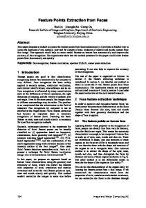
Figure 4.3. Area in which the data was recorded. The image was exported from Google Earth by Brax [3]( ©2010 Tele Atlas, ©2010 Europa Technologies, ©2010 Google, Data SIO, NOAA, U.S. Navy, NGA, GEBCO). Reproduced from Brax [3] with permission.

the raw data. An area well within AIS coverage was selected and all the reports originating from outside this area were discarded, as were duplicates and reports from vessels belonging to ship types other than cargo, tanker and passenger. The area includes the port of Gothenburg with surrounding waters and can be seen in Figure 4.3. Reports belonging to the same vessel were grouped together using the unique identification number present in each report. To reduce the size of the data each trajectory was resampled every 100 meters in case the speed was greater than 0.01 knots or every 60 seconds if the speed was less than 0.01 knots. In the case of two consecutive AIS reports having a time difference greater than 30 minutes the trajectory was split in two. The resulting dataset consists of 8867 trajectories that were split into a training set of size 7980 and an evaluation set size of 887. Two labelled test sets, normal and abnormal, each of size 604 were created using the evaluation set. In this work only a subset of the original abnormal set will be used. The reason for this is that the other 19

CHAPTER 4. FEATURE EXTRACTION FROM MARITIME TRAJECTORIES

anomaly types of the original set involves multiclass anomaly detection. This falls outside the scope of the evaluation of feature spaces. The total size of the abnormal set is therefore reduced to 304 trajectories. The normal test set was obtained by random sampling without replacement form the evaluation set. The abnormal test set and the normal test set can be combined to form five different anomaly test sets, each containing 604 normal trajectories, and either 2 or 100 abnormal trajectories. In other words, we put one anomaly type in each anomaly test set. The abnormal test set trajectories were created in collaboration with subject experts in order to make the trajectories both interesting from an operators perspective as well as realistic. A short description of the five anomaly types present in the abnormal test set can be found below.

4.4.2

Anomaly Types

This is a list with short descriptions of the anomaly types used in the evaluation of the methods described in Section 4.1. Figures 4.4 - 4.8 show the anomalous trajectories plotted against a background of normal traffic trajectories. 1. The circle and land anomaly is based on a real incident in which a ship ran in circles before it eventually ran aground. Thinkable underlying mechanisms for this anomaly include sleeping at the helm and malfunctioning rudder. The anomalies were created by hand, which is a very tedious process, and therefore only two instances were created. 2. The missed turn anomaly is an interpretation of the case of when a ship is following a shipping lane and then fails to turn and is heading towards shallow water. Like the above this anomaly class was manually constructed and only two instances exist. They are located in risk areas where, according to domain experts, ships may miss a turn. 3. The unexpected stop anomaly reflects a situation where a ship comes to a stop for approximately 50 minutes before resuming its route. These anomalies were automatically generated and 100 instances exist. 4. The unusual speed anomaly reflects the situation where a ship suddenly starts to move very slowly or fast. The anomalies were created by randomly selecting a sub-trajectory of length 50 and increase or decrease the speed within the sub-trajectory by 90 % with equal probability. 100 instances of this anomaly type were automatically generated. 5. The strange manoeuvres anomaly corresponds to a sudden streak of erratic course changes before the ship resumes its normal route. It was created by translating each point of a randomly selected sub-trajectory a distance ∆d perpendicular to its current course. ∆d was uniformly sampled from the interval [−500, 500]. The durations of the anomalies were generated by an 20

4.4. DATASET

unknown unimodal distribution with mean 11 minutes and standard deviation 3.7.

21

CHAPTER 4. FEATURE EXTRACTION FROM MARITIME TRAJECTORIES

6

6.42

x 10

6.41

6.4

6.39

6.38

6.37

6.36

−5

−4

−3

−2

−1

0

1 4

x 10

6

x 10

6.396

6.394

6.392

6.39

6.388

6.386

−8000

−6000

−4000

−2000

0

2000

Figure 4.4. Overview (top) and zoomed-in view (bottom) of the two circle and land anomalies, where red and green correspond to the abnormal and normal segments, respectively, and the blue trajectories correspond to the training set. The lengths of the top and bottom abnormal segments are 14 and 38 minutes, respectively. Figure with caption reproduced from Laxhammar [15] with permission.

22

4.4. DATASET 6

6.42

x 10

6.41

6.4

6.39

6.38

6.37

6.36

−5

−4

−3

−2

−1

0

1 4

x 10

6

x 10

6.396

6.394

6.392

6.39

6.388

6.386

6.384

6.382

−10000

−8000

−6000

−4000

−2000

0

2000

Figure 4.5. Overview (top) and zoomed-in view (bottom) of the two missed turn anomalies, where red and green correspond to the abnormal and normal segments, respectively, and the blue trajectories correspond to the training set. The lengths of the left and right abnormal segments are 8 and 15 minutes respectively. Figure with caption reproduced from Laxhammar [15] with permission.

23

CHAPTER 4. FEATURE EXTRACTION FROM MARITIME TRAJECTORIES

6

6.42

x 10

6.41

6.4

6.39

6.38

6.37

6.36

−5

−4

−3

−2

−1

0

1 4

x 10

Figure 4.6. Plot of the 100 anomalous trajectories involved in unexpected stops. red and green correspond to the unexpected stops and the normal segments, respectively, and the blue trajectories correspond to the full training set. Figure with caption reproduced from Laxhammar [15] with permission.

24

4.4. DATASET 6

6.42

x 10

6.41

6.4

6.39

6.38

6.37

6.36

−5

−4

−3

−2

−1

0

1 4

x 10

6

x 10 6.371

6.37

6.369

6.368

6.367

6.366

6.365

6.364

6.363

6.362

6.361

−2.4

−2.2

−2

−1.8

−1.6

−1.4 4

x 10

Figure 4.7. Overview (top) and zoomed-in view (bottom) of two arbitrarily selected trajectories from the set of 100 unusual speed anomalies. Red and green correspond to the abnormal and normal segments, respectively, and the blue trajectories correspond to the full training set. In order to visualise the relative speed of the normal and abnormal segments, the two trajectories have been uniformly sampled in time and the velocity vectors between successive points plotted. Note that the left and right abnormal segments correspond to high-speed and low-speed segments, respectively, which is indicated by the length of the velocity vectors. Figure with caption reproduced from Laxhammar [15] with permission.

25

CHAPTER 4. FEATURE EXTRACTION FROM MARITIME TRAJECTORIES 6

6.42

x 10

6.41

6.4

6.39

6.38

6.37

6.36

−5

−4

−3

−2

−1

0

1 4

x 10

6

x 10

6.374

6.372

6.37

6.368

6.366

6.364

6.362 −2.4

−2.2

−2

−1.8

−1.6

−1.4 4

x 10

Figure 4.8. Overview (top) and zoomed-in view (bottom) of an arbitrarily selected trajectory from the set of 100 strange manoeuvre anomalies. Red and green correspond to the abnormal and normal segments, respectively, and the blue trajectories correspond to the full training set. Figure with caption reproduced from Laxhammar [15] with permission.

26

Chapter 5

Results and Discussion This chapter will present and interpret the results that were obtained through the experiments described in the previous chapter. It begins with a summary of the most important results along with a few illustrative figures and then goes on to a short discussion for each anomaly type.

5.1

Summary of Results

This section is a summary of the results from the evaluation of the proposed feature spaces (Section 4.1) on the dataset described in Section 4.4. In Tables 5.1-5.4 the results of all feature spaces averaged over all anomalies are presented. For a more exhaustive presentation of the results over each individual anomaly type, the reader is referred to Appendix A. In the case of the course only feature all the distance functions mentioned in Section 4.1.3 were evaluated with very similar results. Because they did not prove to be competitive only the results obtained with the distance function given in equation 4.10 are presented. In Figure 5.1, the AUC measured when the Discords algorithm was run on the five different anomaly test sets is presented in a visually more appealing way. The results for pAUC is presented in an identical fashion in Figure 5.2. The results in the figures are for window length w = 11, and time step dt = 30. What motivated that particular parameter choice was that it performed best, averaged over all anomalies and feature spaces in terms of both AUC and pAUC, although closely followed by w = 3, dt = 30. Finally, all feature spaces have been evaluated with the parameter setting with which they on average performed best. The results are presented in Figure 5.3 and the exact results and parameter settings can be found in Table 5.5. 27

CHAPTER 5. RESULTS AND DISCUSSION Table 5.1. Mean AUC

spa 0.836 0.879 0.863 0.843 0.799

w = 3, dt = 30 w = 11, dt = 30 w = 11, dt = 60 w = 11, dt = 120 w = 11, dt = 180

vel 0.928 0.937 0.919 0.893 0.814

spavel 0.960 0.959 0.952 0.927 0.829

spaspe 0.961 0.927 0.905 0.885 0.824

spe 0.901 0.890 0.874 0.884 0.801

dir 0.721 0.721 0.751 0.740 0.688

relspa 0.926 0.922 0.907 0.866 0.876

dir 0.032 0.073 0.134 0.120 0.005

relspa 0.423 0.492 0.392 0.311 0.175

dir 0.054 0.132 0.180 0.226 0.012

relspa 0.656 0.616 0.442 0.346 0.220

Table 5.2. Mean Partial AUC for f pr ∈ (0, 0.01)

spa 0.402 0.301 0.212 0.119 0.162

w = 3, dt = 30 w = 11, dt = 30 w = 11, dt = 60 w = 11, dt = 120 w = 11, dt = 180

vel 0.344 0.396 0.405 0.291 0.267

spavel 0.381 0.465 0.385 0.283 0.229

spaspe 0.343 0.380 0.507 0.352 0.385

spe 0.319 0.274 0.229 0.255 0.303

Table 5.3. Mean Sensitivity (tpr) for f pr = 0.01

w = 3, dt = 30 w = 11, dt = 30 w = 11, dt = 60 w = 11, dt = 120 w = 11, dt = 180

spa 0.402 0.418 0.250 0.182 0.222

vel 0.708 0.538 0.488 0.328 0.306

spavel 0.608 0.698 0.462 0.330 0.340

spaspe 0.640 0.542 0.662 0.500 0.474

spe 0.652 0.458 0.316 0.372 0.362

Table 5.4. Average Mean detection delay (seconds) for f pr = 0.01

w = 3, dt = 30 w = 11, dt = 30 w = 11, dt = 60 w = 11, dt = 120 w = 11, dt = 180

5.2

spa 338 2076 1332 1569 1456

vel 188 151 407 767 1340

spavel 90 287 340 697 1481

spaspe 277 225 382 471 621

spe 314 211 234 485 559

dir 1561 -888 454 8611 1120

relspa 247 180 549 817 1265

Anomaly Types Revisited

This section will go through each anomaly type and highlight the most interesting parts of the results that were presented in the previous section. Not only the best results are considered interesting, but also those that do not agree well with what was expected. 28

5.2. ANOMALY TYPES REVISITED

1 0.9 0.8 0.7

AUC

0.6 0.5 0.4 0.3 Spatial Velocity SpatialAndVelocity SpatialAndSpeed Speed Course RelativeSpatial

0.2 0.1

cl c ir

n ea

0 a nd dl

t ur ed s s mi

n u

p ne x

ec

sto ted

p

e l sp a u s u nu

ed str

a

ng e

ma

eu no

vre

Figure 5.1. Plot of AUC performance for each feature space over all anomaly types. The dashed line marks the performance of a random classifier. Parameters used were w = 11 and dt = 30.

5.2.1

Circle and Land

The circle and land anomaly type was the one on which the best classification performance, in terms of pAUC, was reached. While that might suggest that it is an easy anomaly to detect there is one important factor to consider before that conclusion is drawn. As was described in Section 4.4.2, there exists only two instances of this anomaly type because it was hand-crafted in a very time-consuming manner. This has an unfortunate but inevitable impact on the reliability of the results. Furthermore a qualitative analysis of the two anomalies we have can say something about how well the obtained results are likely to generalize. The two anomalous tracks quite quickly venture out into areas where there is no training data, as can be seen in Figure 4.4. This makes the tracks easy to pick up by the spatial feature with the shortest possible window length without taking into account the anomalous circular behavior. It can be seen Figures 5.1 - 5.3 that the spatial feature indeed performs well on this anomaly. Though, as was described in Section 4.4.2, the real world inspiration for this anomaly type was a grounding incident. Because 29

CHAPTER 5. RESULTS AND DISCUSSION

1 Spatial Velocity SpatialAndVelocity SpatialAndSpeed Speed Course RelativeSpatial

0.9 0.8 0.7

pAUC

0.6 0.5 0.4 0.3 0.2 0.1

cl c ir

n ea

0 a nd dl

t ur ed s s mi

n u

p ne x

ec

sto ted

p

e l sp a u s u nu

ed str

a

ng e

ma

eu no

vre

Figure 5.2. Plot of pAUC performance for each feature space over all anomaly types. The dashed line marks the performance of a random classifier. Parameters used were w = 11 and dt = 30.

ships are unlikely to have previously traveled in very shallow water, there may be some merit to the method of only considering the ships position. However, the relative spatial feature space performed very well on this anomaly. In contrast to the spatial feature space it is impossible for the algorithm to detect that the ship is traveling where no other ship has traveled before. Therefore it can be concluded that the relative spatial feature space was indeed able to detect the circular behavior of this anomaly type. The same analysis can largely be made about the velocity only feature space as well, even though it did not perform at quite the same level. Surprisingly, this anomaly proved to be the Achilles heel of the spatial and speed combination feature space. With two thirds of the feature space being made up of the spatial features it was expected to perform reasonably well, and at least as well as the spatial and velocity feature space. Although very few anomaly samples were tested this can be seen as a first indication of the limitations of this feature space. Fortunately there is one easy way to remedy the inadequacy of the few anomaly 30

5.2. ANOMALY TYPES REVISITED

1 0.9 0.8 0.7 Spatial Velocity SpatialAndVelocity SpatialAndSpeed Speed Course RelativeSpatial

pAUC

0.6 0.5 0.4 0.3 0.2 0.1

cl c ir

n ea

0 a nd dl

m

t ur ed is s

n u

p ne x

ec

sto ted

p

e l sp a u s u nu

ed str

a

ng e

ma

eu no

vre

Figure 5.3. Plot of pAUC performance for each feature space over all anomaly types. The dashed line marks the performance of a random classifier. The parameters w and dt were optimized so that each feature space was evaluated with the parameters with which it performed best on average. The exact performance and parameters for each feature space can be seen in Table 5.5.

Table 5.5. Partial AUC for f pr ∈ (0, 0.01) and optimized parameters

circle and land missed turn unexpected stop unusual speed strange manoeuvre

spa w=3 dt = 30 1.000 1.000 0.000 0.010 0.000

vel w = 11 dt = 60 1.000 0.000 0.086 0.246 0.691

spavel w = 11 dt = 30 0.857 0.143 0.254 0.321 0.747

31

spaspe w = 11 dt = 60 0.286 0.286 0.716 0.801 0.444

spe w=3 dt = 30 0.214 0.214 0.354 0.426 0.387

dir w = 11 dt = 60 0.429 0.000 0.001 0.010 0.229

relspa w = 11 dt = 30 1.000 0.000 0.249 0.540 0.671

CHAPTER 5. RESULTS AND DISCUSSION

samples, and that is to evaluate on a larger set of circle and land anomalies. To avoid the time-consuming process of crafting the anomalies by hand it should be possible to automatically generate a large number of anomalies. This is an issue that we will come back to.

5.2.2

Missed Turn

The missed turn anomaly type has two things in common with the circle and land anomaly type. Both have only two instances for the same reason, and all four anomaly tracks quickly venture far from any training data in the spatial space. As with the circle and land anomaly type, this leads to good performance for the spatial feature. The most important difference between the two anomaly types is that the missed turn has no anomalous circling behavior. This absence is likely what causes the poor performance of all the relative feature spaces in terms of pAUC, including relative spatial, velocity, and course feature spaces.

5.2.3

Unexpected Stop

It was previously suggested in this work that feature spaces that consist only of positions or velocities should not be the best for detecting unexpected stops. This was one of the motivations for creating the combination feature spaces. As can be seen in Figure 5.1 and more clearly in Figure 5.2 the combination feature spaces do indeed perform better than the separate spatial and velocity features. In particular, the spatial and speed feature performed clearly better than the rest. A bit surprisingly the relative spatial features performed about as good as the spatial and velocity feature, and the speed only feature even performed slightly better. It should perhaps be noted that the second best pAUC performance after spatial and speed feature was the spatial feature with the longest tested sliding window, w = 11 and dt = 180 (see Appendix A). However, this parameter setting was not particularly good with the other anomalies, especially not the circle and land and missed turn anomalies, in which the spatial feature excelled with shorter window lengths. That the spatial feature performed badly on this anomaly with its on average best sliding window parameters can be clearly seen in Figure 5.3.

5.2.4

Unusual Speed

There is a description in Section 4.4.2 of how the unusual speed anomaly test set was created by randomly selecting sub-trajectories and altering their speed, either increasing or decreasing it. This random selection process should ensure that the probability of anomalous speed is not conditionally dependent on position. In other words, the position alone should not contain any information as to whether a trajectory has an anomalous speed or not. This is enough to give rise to the suspicion that the spatial feature space might not be very effective at detecting this anomaly. Especially not at short sliding window lengths where the absolute position of the 32

5.2. ANOMALY TYPES REVISITED

trajectory dominate the movement. When the results, e.g. in Figure 5.3, are considered we can conclude that spatial feature indeed proved to be inferior to the other measures at detecting this anomaly. Instead, it was expected that better results should come from the relative feature spaces, i.e. the relative spatial, the speed and the velocity. However, while they performed much better than the spatial feature space, it was the spatial and speed feature space that was clearly best. In addition, the result that the spatial data contributed to the classification performance is consistent in the sense that the spatial and velocity feature space was better than velocity with their optimal parameter settings, see Figure 5.3. A possible explanation for these results goes back to the speed distribution in the data and the way that the anomaly type was created. The explanation has to do with the normal distribution of the speed which is dependent on the position of a ship. Specifically, ships, on average, move slower in the port area. One reason for that is that they anchor and perform complex manoeuvres there but there is also a speed limit which has an impact on the speed distribution. In this respect, the unusual speed anomaly type is very similar to the previously covered unexpected stop anomaly type. The combination feature spaces allow a ship moving very slowly in the open sea to be classified as an anomaly even though a low speed is normal in the port area. Of course it also works the other way, if a ship is moving fast in the port area, or at least significantly above the speed limit, it may be classified as an anomaly even though it may be a moderate speed at open sea.

5.2.5

Strange Manoeuvre

The strange manoeuvre anomaly type is similar to the unusual speed in that the spatial feature space was expected to perform badly. The logic behind the expectation is that while the artificial anomaly had the positions of each trajectory sample changed, see Figure 4.8, it never moved them far enough to deviate significantly from the sea lanes. Just like in the case of the unusual speed anomaly the expectation was that the relative feature spaces should perform better than the purely spatial and as can be seen in Figures 5.2-5.3, they did. What is different from the unusual speed anomaly type is that it was not expected that the combination feature spaces should perform any better than the velocity and relative spatial feature spaces. However, the pattern from the unusual speed anomaly type repeats itself, the spatial and velocity is better than velocity and the spatial and speed is better than speed. While this was surprising the difference is not as big as in the unusual speed case. There is one aspect of the results in the strange manoeuvre anomaly type that is very peculiar; the speed only feature space shows decent performance. According to how the data was created there is no obvious reason for this. The speed is not supposed to be altered at all in this anomaly which suggests it should perform along the lines of a random classifier, but it does not. This raised the suspicion 33

CHAPTER 5. RESULTS AND DISCUSSION

12

10

Speed (m /s)

8

6

4

2

0 0

1000

2000

3000

4000 5000 T im e (s)

6000

7000

8000

Figure 5.4. The speed of a randomly selected trajectory from the strange manoeuvre data set is plotted against time. The anomalous part (red) does not seem to significantly differ from the normal part (green).

that the speed of the trajectories had been inadvertently altered when the strange manoeuvre anomalies were created. However, when the speed of the anomalous trajectories is examined, see Figure 5.4, it becomes clear that the explanation is not that simple. What causes the speed feature space to perform as well as it does remains unknown but it is likely that further analysis of the data will result in the discovery of some inconsistency in the speed. The strange manoeuvre and circle and land anomaly types were the only ones which the course feature space showed any promise at all. However, to be fair, they are also the only ones that can be expected to be anomalous in the course feature space, because they are the only ones that involve any turning. Even though the course only feature is so specific that it can only capture these two anomalies, it still performed much worse than the other feature spaces.

5.2.6

Summary

By looking at the optimized results in Figure 5.3 and Table 5.5 it can be concluded that no single feature space has very good performance across all anomaly types. 34

5.2. ANOMALY TYPES REVISITED

The best feature space for the two first anomaly types is clearly the spatial only with a short window length. It is likely that for those anomaly spaces the performance would be even better if we considered a point feature space, i.e. f = (x, y), for the dominating factor seems to be the absolute position of the ship. The last three anomaly types were, on average, best tackled by the spatial and speed feature space. This is also the feature space that scored the best average over all anomaly types in terms of pAUC, see Table 5.1. However, in terms of sensitivity, the spatial and velocity feature space was the best, also Table 5.1. This proves our previous argument that not only are the measures we use on our data important, but the measures we use to evaluate those measures are important as well (Section 4.3).

35

Chapter 6

Conclusions This is the final chapter in which we discuss the main conclusions that can be drawn from this work. We also discuss how the work may be used in a live anomaly detector and some potential future work.

6.1

Contributions

In this work a total of seven feature spaces have been evaluated within the context of anomaly detection in maritime trajectories. The ones that performed the best were the ordinary spatial only feature space that is widely used in the literature, but also the spatial and speed feature space which has been proposed in this thesis. To our knowledge, no one has used this particular feature space before even though it is very easily implemented. The two feature spaces seem to complement each other reasonably well, an observation that might be of importance for future work, but more will be said on this in the next section.

6.2

Further Research

While this work has given some new insights, much remains to be done. For one, the evaluation of the feature space would benefit from the use of real anomaly data instead of the synthetic anomalies that were used in this work. The obvious problem with the collection of real anomalous data is that anomalies are scarce. Therefore, another approach may be to improve the way that the synthetic data is generated. It would be best if the generating process is a physically consistent simulation of a ship performing manoeuvres corresponding to the five anomaly types that were used in this work. This would reduce the occurrence of instantaneous speed changes, i.e. infinite accelerations, and other physically impossible phenomenon in the data. The two hand-crafted anomaly types, the circle and land and missed turn, would of course benefit the most as the number of examples could be drastically increased. Another promising lead for improved anomaly detection performance is the simultaneous usage of two or more of the feature spaces. As was mentioned in Section 37

CHAPTER 6. CONCLUSIONS

5.2.6, the spatial and the spatial and speed feature spaces complement each other reasonably well. This can be taken as a sign that two nonconformity measures, each utilizing one of those feature spaces, could potentially achieve a better overall performance than anything that has been proposed so far. The effects of the combination of two nonconformity measures, possibly in a hierarchical manner, must be examined. For instance, what will the implications be on the well-tuned alarm rate otherwise inherently present in conformal anomaly detectors? To be explored is also the possibility of scaling the different parts of a feature space. In the case of the spatial and speed anomaly this would mean that we scale the speed up or down by a certain amount that could be optimized through crossvalidation. In this work we just assumed that all the different components should be equally scaled to a mean of zero and a variance of one. A more systematic approach to this issue would be very welcome.

6.3

Final Remarks

The development of a maritime trajectory anomaly detector is likely a long process. Careful consideration must be given to which types of anomalies are most important to detect as this decision will have a big impact on what methods are best suited to the task. This is probably best done in collaboration with the operators which will utilize the system once it has been constructed. In the case of conformal anomaly detection this means the selection of the most appropriate nonconformity measure, but also the features which we plug into it. It is our hope that this work has contributed to the understanding of the importance of the selection of the feature space in the construction of anomaly detectors in the specific, and machine learning in general.

38

Bibliography [1]

V. Avram. A spatio-temporal data representation framework with applications to anomaly detection in the maritime domain. Master’s thesis, Simon Fraser University, 2012.

[2]

S. Axelsson. The base-rate fallacy and the difficulty of intrusion detection. ACM Transactions on Information and System Security (TISSEC), 3(3):185– 205, August 2000.

[3]

C. Brax. Anomaly Detection in the Surveillance Domain. PhD thesis, Örebro University, 2011.

[4]

V. Chandola, A. Banerjee, and V. Kumar. Anomaly detection: A survey. ACM Computing Surveys, 41(3):1–58, 2009.

[5]

Lei Chen, M. Tamer Özsu, and Vincent Oria. Robust and fast similarity search for moving object trajectories. In Proceedings of the 2005 ACM SIGMOD International Conference on Management of Data, SIGMOD ’05, pages 491– 502, New York, NY, USA, 2005. ACM.

[6]

Jan Ekman and Anders Holst. Anomaly detection in vessel motion. Internal Report, 2003.

[7]

T. Fawcett. An introduction to ROC analysis. Pattern Recognition Letters Special issue: ROC analysis in pattern recognition, 27(8):861–874, June 2006.

[8]

A. Gammerman and V. Vovk. Hedging predictions in machine learning. The Computer Journal, 50(2):151–163, 2007.

[9]

Alexander Gammerman, Volodya Vovk, and Vladimir Vapnik. Learning by transduction. In Proceedings of the Fourteenth conference on Uncertainty in artificial intelligence, pages 148–155. Morgan Kaufmann Publishers Inc., 1998.

[10] D. Hawkins. Identification of Outliers. Chapman and Hall, London, 1980. [11] Hye-Young Kang, Joon-Seok Kim, and Ki-Joune Li. Similarity measures for trajectory of moving objects in cellular space. In Proceedings of the 2009 ACM Symposium on Applied Computing, SAC ’09, pages 1325–1330, New York, NY, USA, 2009. ACM. 39

BIBLIOGRAPHY

[12] E. Keogh, J. Lin, and A. Fu. Hot sax: Efficiently finding the most unusual time series subsequence. In Proceedings of the 5th IEEE International Conference on Data Mining, 2005. [13] R. Laxhammar, G. Falkman, and E. Sviestins. Anomaly detection in sea traffic a comparison of the gaussian mixture model and the kernel density estimator. In Proceedings of the 12th International Conference on Information Fusion, pages 756–763, Seattle, USA, July 2009. [14] Rikard Laxhammar. Anomaly detection for sea surveillance. In Proceedings of the 11th International Conference on Information Fusion, pages 1–8, Cologne, Germany, July 2008. [15] Rikard Laxhammar. Conformal Anomaly Detection. PhD thesis, University of Skövde, 2014. [16] Hua Ma, Andriy I. Bandos, Howard E. Rockette, and David Gur. On use of partial area under the roc curve for evaluation of diagnostic performance. Statistics in Medicine, 32(20):3449–3458, 2013. [17] Donna Katzman McClish. Analyzing a portion of the roc curve. Medical Decision Making, 9(3):190–195, August 1989. [18] Commission of the European Communities. Common position adopted by the council on 6 june 2008 with a view to the adoption of a directive of the european parliament and of the council amending directive 2002/59/ec establishing a community vessel traffic monitoring and information system, 2008. [19] International Maritime Organization. International Convention for the Safety of Life at Sea (SOLAS), Chapter V: Safety of Navigation, Regulation 19, 2002. [20] G. Pallotta, M. Vespe, and K. Bryan. Vessel pattern knowledge discovery from ais data: A framework for anomaly detection and route prediction. Entropy, 15:2218–2245, 2013. [21] C. Piciarelli and G.L. Foresti. On-line trajectory clustering for anomalous events detection. Pattern Recognition Letters - Special issue on vision for crime detection and prevention, 27, 2006. [22] Thanawin Rakthanmanon, Bilson Campana, Abdullah Mueen, Gustavo Batista, Brandon Westover, Qiang Zhu, Jesin Zakaria, and Eamonn Keogh. Searching and mining trillions of time series subsequences under dynamic time warping. In Proceedings of the 18th ACM SIGKDD International Conference on Knowledge Discovery and Data Mining, KDD ’12, pages 262–270, New York, NY, USA, 2012. ACM. 40

BIBLIOGRAPHY

[23] B.J. Rhodes, N.A. Bomberger, and M. Zandipour. Probabilistic associative learning of vessel motion patterns at multiple scales for maritime situation awareness. In Proceedings of the 10th International Conference on Information Fusion, Quebec, Canada, July 2007. [24] G. Shafer and V. Vovk. A Tutorial on Conformal Prediction. Journal of Machine Learning Research, 9:371–421, March 2008. [25] Marc van Kreveld and Jun Luo. The definition and computation of trajectory and subtrajectory similarity. In Proceedings of the 15th Annual ACM International Symposium on Advances in Geographic Information Systems, GIS ’07, pages 44:1–44:4, New York, NY, USA, 2007. ACM. [26] M. Vlachos, G. Kollios, and D. Gunopoulos. Discovering similar multidimensional trajectories. In Proceedings of the 18th IEEE International Conference on Data Engineering, 2002. [27] V. Vovk, A. Gammerman, and G. Shafer. Algorithmic Learning in a Random World. Springer-Verlag New York, Inc., Secaucus, NJ, USA, 2005. [28] Xiaoyue Wang, Abdullah Mueen, Hui Ding, Goce Trajcevski, Peter Scheuermann, and Eamonn Keogh. Experimental comparison of representation methods and distance measures for time series data. Data Mining and Knowledge Discovery, 26(2):275–309, 2013. [29] Jian-Xin Zeng, Hui-Li Gong, Ting Liu, Yue Men, and Ning Yang. Comparing and analysing three kinds of conformal predictor. In Fuzzy Systems and Knowledge Discovery (FSKD), 2012 9th International Conference on, pages 684–688, May 2012. [30] Z. Zhang, K. Huang, and Tan T. Comparison of similarity measures for trajectory clustering in outdoor surveillance scenes. In Proceedings of 18th International Conference on Pattern Recognition (ICPR), 2006.

41

Appendix A

Additional Tables

43

APPENDIX A. ADDITIONAL TABLES

A.1

Circle and Land

Table A.1. AUC

w = 3, dt = 30 w = 11, dt = 30 w = 11, dt = 60 w = 11, dt = 120 w = 11, dt = 180

spa 1.000 0.998 0.992 0.988 0.969

vel 0.996 0.998 1.000 1.000 0.999

spavel 0.997 0.998 1.000 1.000 0.998

spaspe 0.976 0.923 0.944 0.985 0.993

spe 0.878 0.772 0.860 0.982 0.985

dir 0.925 0.950 0.988 0.994 0.954

relspa 0.997 1.000 1.000 1.000 0.992

dir 0.000 0.000 0.429 0.500 0.000

relspa 0.714 1.000 1.000 1.000 0.500

dir 0.000 0.000 0.500 1.000 0.000

relspa 1.000 1.000 1.000 1.000 0.500

Table A.2. Partial AUC for f pr ∈ (0, 0.01)

w = 3, dt = 30 w = 11, dt = 30 w = 11, dt = 60 w = 11, dt = 120 w = 11, dt = 180

spa 1.000 0.857 0.429 0.357 0.357

vel 0.643 0.857 1.000 1.000 0.929

spavel 0.714 0.857 1.000 1.000 0.786

spaspe 0.143 0.000 0.286 0.143 0.429

spe 0.214 0.000 0.000 0.286 0.500

Table A.3. Sensitivity (tpr) for f pr = 0.01

w = 3, dt = 30 w = 11, dt = 30 w = 11, dt = 60 w = 11, dt = 120 w = 11, dt = 180

spa 1.000 1.000 0.500 0.500 0.500

vel 1.000 1.000 1.000 1.000 1.000

spavel 1.000 1.000 1.000 1.000 1.000

spaspe 0.500 0.000 0.500 0.500 0.500

spe 0.500 0.000 0.000 0.500 0.500

Table A.4. Mean detection delay (seconds) for f pr = 0.01

w = 3, dt = 30 w = 11, dt = 30 w = 11, dt = 60 w = 11, dt = 120 w = 11, dt = 180

spa 732 702 791 1691 2111

vel 237 267 267 267 267

spavel 267 267 267 267 267 44

spaspe 733 NaN 703 643 403

spe 703 NaN NaN 403 43

dir NaN NaN 643 1167 NaN

relspa 282 297 327 447 671

A.2. MISSED TURN

A.2

Missed Turn

Table A.5. AUC

w = 3, dt = 30 w = 11, dt = 30 w = 11, dt = 60 w = 11, dt = 120 w = 11, dt = 180

spa 1.000 0.995 0.964 0.895 0.725

vel 0.775 0.824 0.761 0.734 0.435

spavel 0.923 0.916 0.911 0.893 0.498

spaspe 0.921 0.799 0.689 0.622 0.354

spe 0.746 0.790 0.675 0.703 0.372

dir 0.488 0.480 0.533 0.474 0.351

relspa 0.804 0.741 0.714 0.644 0.803

dir 0.000 0.000 0.000 0.000 0.000

relspa 0.286 0.000 0.000 0.000 0.000

dir 0.000 0.000 0.000 0.000 0.000

relspa 0.500 0.000 0.000 0.000 0.000

Table A.6. Partial AUC for f pr ∈ (0, 0.01)

w = 3, dt = 30 w = 11, dt = 30 w = 11, dt = 60 w = 11, dt = 120 w = 11, dt = 180

spa 1.000 0.571 0.500 0.000 0.000

vel 0.071 0.000 0.000 0.000 0.000

spavel 0.000 0.143 0.000 0.000 0.000

spaspe 0.214 0.357 0.286 0.000 0.000

spe 0.214 0.286 0.000 0.000 0.000

Table A.7. Sensitivity (tpr) for f pr = 0.01

w = 3, dt = 30 w = 11, dt = 30 w = 11, dt = 60 w = 11, dt = 120 w = 11, dt = 180

spa 1.000 1.000 0.500 0.000 0.000

vel 0.500 0.000 0.000 0.000 0.000

spavel 0.000 0.500 0.000 0.000 0.000

spaspe 0.500 0.500 0.500 0.000 0.000

spe 0.500 0.500 0.000 0.000 0.000

Table A.8. Mean detection delay (seconds) for f pr = 0.01

w = 3, dt = 30 w = 11, dt = 30 w = 11, dt = 60 w = 11, dt = 120 w = 11, dt = 180

spa 241 331 393 NaN NaN

vel 663 NaN NaN NaN NaN

spavel NaN 693 NaN NaN NaN 45

spaspe 573 603 573 NaN NaN

spe 603 633 NaN NaN NaN

dir NaN NaN NaN NaN NaN

relspa 603 NaN NaN NaN NaN

APPENDIX A. ADDITIONAL TABLES

A.3

Unexpected Stop

Table A.9. AUC

w = 3, dt = 30 w = 11, dt = 30 w = 11, dt = 60 w = 11, dt = 120 w = 11, dt = 180

spa 0.623 0.813 0.856 0.885 0.898

vel 0.924 0.922 0.907 0.903 0.898

spavel 0.935 0.936 0.931 0.927 0.926

spaspe 0.961 0.962 0.960 0.951 0.949

spe 0.943 0.948 0.921 0.903 0.884

dir 0.672 0.661 0.723 0.793 0.807

relspa 0.887 0.921 0.918 0.907 0.900

dir 0.010 0.004 0.001 0.009 0.000

relspa 0.163 0.249 0.251 0.230 0.211

dir 0.010 0.010 0.000 0.010 0.000

relspa 0.280 0.410 0.290 0.300 0.300

Table A.10. Partial AUC for f pr ∈ (0, 0.01)

w = 3, dt = 30 w = 11, dt = 30 w = 11, dt = 60 w = 11, dt = 120 w = 11, dt = 180

spa 0.000 0.009 0.043 0.190 0.384

vel 0.175 0.096 0.086 0.157 0.184

spavel 0.291 0.254 0.176 0.224 0.254

spaspe 0.517 0.539 0.716 0.666 0.669

spe 0.354 0.250 0.270 0.317 0.346

Table A.11. Sensitivity (tpr) for f pr = 0.01

w = 3, dt = 30 w = 11, dt = 30 w = 11, dt = 60 w = 11, dt = 120 w = 11, dt = 180

spa 0.000 0.010 0.130 0.330 0.510

vel 0.420 0.220 0.180 0.210 0.220

spavel 0.630 0.510 0.280 0.340 0.460

spaspe 0.750 0.750 0.800 0.740 0.740

spe 0.700 0.490 0.380 0.450 0.440

Table A.12. Mean detection delay (seconds) for f pr = 0.01

w = 3, dt = 30 w = 11, dt = 30 w = 11, dt = 60 w = 11, dt = 120 w = 11, dt = 180

spa NaN 7014 1491 1372 1177

vel -2 179 845 1289 1589

spavel 3 301 452 763 1120 46

spaspe -4 32 90 355 554

spe 5 22 205 410 700

dir 2969 -3501 NaN 24005 NaN

relspa 233 141 1029 1611 1859

A.4. UNUSUAL SPEED

A.4

Unusual Speed

Table A.13. AUC

spa 0.699 0.789 0.777 0.743 0.708

w = 3, dt = 30 w = 11, dt = 30 w = 11, dt = 60 w = 11, dt = 120 w = 11, dt = 180

vel 0.954 0.948 0.935 0.868 0.836

spavel 0.956 0.949 0.934 0.866 0.830

spaspe 0.968 0.964 0.958 0.899 0.877

spe 0.959 0.953 0.944 0.893 0.875

dir 0.541 0.530 0.538 0.540 0.538

relspa 0.953 0.953 0.937 0.878 0.821

dir 0.001 0.019 0.010 0.020 0.006

relspa 0.401 0.540 0.476 0.273 0.131

dir 0.010 0.030 0.010 0.030 0.020

relspa 0.650 0.710 0.560 0.340 0.230

Table A.14. Partial AUC for f pr ∈ (0, 0.01)

spa 0.010 0.061 0.077 0.033 0.051

w = 3, dt = 30 w = 11, dt = 30 w = 11, dt = 60 w = 11, dt = 120 w = 11, dt = 180

vel 0.334 0.319 0.246 0.176 0.177

spavel 0.286 0.321 0.179 0.119 0.076

spaspe 0.478 0.601 0.801 0.649 0.531

spe 0.426 0.491 0.593 0.553 0.550

Table A.15. Sensitivity (tpr) for f pr = 0.01

w = 3, dt = 30 w = 11, dt = 30 w = 11, dt = 60 w = 11, dt = 120 w = 11, dt = 180

spa 0.010 0.070 0.100 0.050 0.080

vel 0.700 0.520 0.410 0.230 0.230

spavel 0.530 0.530 0.250 0.190 0.170

spaspe 0.780 0.830 0.910 0.760 0.690

spe 0.800 0.700 0.750 0.690 0.690

Table A.16. Mean detection delay (seconds) for f pr = 0.01

w = 3, dt = 30 w = 11, dt = 30 w = 11, dt = 60 w = 11, dt = 120 w = 11, dt = 180

spa 41 123 1376 924 1505

vel 70 66 143 422 2025

spavel 52 83 253 1118 1353 47

spaspe -62 75 147 352 447

spe 61 39 335 250 370

dir 1087 286 161 8302 3956

relspa 62 106 169 336 883

APPENDIX A. ADDITIONAL TABLES

A.5

Strange Manoeuvre Table A.17. AUC

w = 3, dt = 30 w = 11, dt = 30 w = 11, dt = 60 w = 11, dt = 120 w = 11, dt = 180

spa 0.859 0.800 0.727 0.701 0.697

vel 0.990 0.994 0.990 0.957 0.903

spavel 0.990 0.993 0.985 0.947 0.893

spaspe 0.980 0.987 0.976 0.967 0.947

spe 0.979 0.985 0.971 0.941 0.891

dir 0.979 0.985 0.974 0.899 0.790

relspa 0.990 0.993 0.969 0.903 0.863

dir 0.146 0.344 0.229 0.070 0.017

relspa 0.550 0.671 0.231 0.054 0.030

dir 0.250 0.620 0.390 0.090 0.040

relspa 0.850 0.960 0.360 0.090 0.070

Table A.18. Partial AUC for f pr ∈ (0, 0.01)

w = 3, dt = 30 w = 11, dt = 30 w = 11, dt = 60 w = 11, dt = 120 w = 11, dt = 180

spa 0.000 0.004 0.013 0.016 0.017

vel 0.499 0.707 0.691 0.120 0.047

spavel 0.616 0.747 0.569 0.070 0.030

spaspe 0.364 0.404 0.444 0.300 0.296

spe 0.387 0.343 0.284 0.120 0.117

Table A.19. Sensitivity (tpr) for f pr = 0.01

w = 3, dt = 30 w = 11, dt = 30 w = 11, dt = 60 w = 11, dt = 120 w = 11, dt = 180

spa 0.000 0.010 0.020 0.030 0.020

vel 0.920 0.950 0.850 0.200 0.080

spavel 0.880 0.950 0.780 0.120 0.070

spaspe 0.670 0.630 0.600 0.500 0.440

spe 0.760 0.600 0.450 0.220 0.180

Table A.20. Mean detection delay (seconds) for f pr = 0.01

w = 3, dt = 30 w = 11, dt = 30 w = 11, dt = 60 w = 11, dt = 120 w = 11, dt = 180

spa NaN 2210 2608 2291 1033

vel -29 92 371 1092 1481

spavel 39 92 386 642 3185

48

spaspe 146 191 397 534 1081

spe 200 151 164 879 1125

dir 627 551 557 971 -1716

relspa 57 177 671 875 1645