Feature Extraction and Image Processing

Dedication We would like to dedicate this book to our parents. To Gloria and to Joaquin Aguado, and to Brenda and the late Ian Nixon.

Feature Extraction and Image Processing Mark S. Nixon Alberto S. Aguado

Newnes OXFORD AUCKLAND BOSTON JOHANNESBURG MELBOURNE NEW DELHI

Newnes An imprint of Butterworth-Heinemann Linacre House, Jordan Hill, Oxford OX2 8DP 225 Wildwood Avenue, Woburn, MA 01801-2041 A division of Reed Educational and Professional Publishing Ltd A member of the Reed Elsevier plc group First edition 2002 © Mark S. Nixon and Alberto S. Aguado 2002 All rights reserved. No part of this publication may be reproduced in any material form (including photocopying or storing in any medium by electronic means and whether or not transiently or incidentally to some other use of this publication) without the written permission of the copyright holder except in accordance with the provisions of the Copyright, Designs and Patents Act 1988 or under the terms of a licence issued by the Copyright Licensing Agency Ltd, 90 Tottenham Court Road, London, England W1P 0LP. Applications for the copyright holder’s written permission to reproduce any part of this publication should be addressed to the publishers British Library Cataloguing in Publication Data A catalogue record for this book is available from the British Library ISBN 0 7506 5078 8 Typeset at Replika Press Pvt Ltd, Delhi 110 040, India Printed and bound in Great Britain

Preface .......................................................................

ix

Why did we write this book? ......................................... The book and its support .............................................. In gratitude .................................................................... Final message ..............................................................

ix x xii xii

1 Introduction ............................................................

1

1.1 Overview ................................................................. 1.2 Human and computer vision ................................... 1.3 The human vision system ....................................... 1.4 Computer vision systems ....................................... 1.5 Mathematical systems ............................................ 1.6 Associated literature ............................................... 1.7 References .............................................................

1 1 3 10 15 24 28

2 Images, sampling and frequency domain processing .................................................................

31

2.1 Overview ................................................................. 2.2 Image formation...................................................... 2.3 The Fourier transform ............................................. 2.4 The sampling criterion ............................................ 2.5 The discrete Fourier transform ( DFT) .................... 2.6 Other properties of the Fourier transform ............... 2.7 Transforms other than Fourier ................................ 2.8 Applications using frequency domain properties .... 2.9 Further reading ....................................................... 2.10 References ...........................................................

31 31 35 40 45 53 57 63 65 65

3 Basic image processing operations ....................

67

3.1 Overview ................................................................. 3.2 Histograms ............................................................. 3.3 Point operators ....................................................... 3.4 Group operations .................................................... 3.5 Other statistical operators....................................... 3.6 Further reading ....................................................... 3.7 References .............................................................

67 67 69 79 88 95 96

4 Low- level feature extraction ( including edge detection) ...................................................................

99

4.1 Overview ................................................................. 4.2 First-order edge detection operators ...................... 4.3 Second- order edge detection operators ................ 4.4 Other edge detection operators .............................. 4.5 Comparison of edge detection operators ............... 4.6 Detecting image curvature ...................................... 4.7 Describing image motion ........................................ 4.8 Further reading ....................................................... 4.9 References .............................................................

99 99 120 127 129 130 145 156 157

5 Feature extraction by shape matching ................

161

5.1 Overview ................................................................. 5.2 Thresholding and subtraction ................................. 5.3 Template matching ................................................. 5.4 Hough transform (HT)............................................. 5.5 Generalised Hough transform (GHT) ..................... 5.6 Other extensions to the HT ..................................... 5.7 Further reading ....................................................... 5.8 References .............................................................

161 162 164 173 199 213 214 214

6 Flexible shape extraction ( snakes and other techniques) ................................................................

217

6.1 Overview ................................................................. 6.2 Deformable templates ............................................ 6.3 Active contours (snakes) ........................................ 6.4 Discrete symmetry operator ................................... 6.5 Flexible shape models ............................................ 6.6 Further reading ....................................................... 6.7 References .............................................................

217 218 220 236 240 243 243

7 Object description .................................................

247

7.1 Overview ................................................................. 7.2 Boundary descriptions ............................................ 7.3 Region descriptors .................................................. 7.4 Further reading .......................................................

247 248 278 288

7.5 References .............................................................

288

8 Introduction to texture description, segmentation and classification .............................

291

8.1 Overview ................................................................. 8.2 What is texture?...................................................... 8.3 Texture description ................................................. 8.4 Classification .......................................................... 8.5 Segmentation ......................................................... 8.6 Further reading ....................................................... 8.7 References .............................................................

291 292 294 301 306 307 308

Appendices................................................................

311

9.1 Appendix 1: Homogeneous co-ordinate system ..... 9.2 Appendix 2: Least squares analysis ....................... 9.3 Appendix 3: Example Mathcad worksheet for Chapter 3 ...................................................................... 9.4 Appendix 4: Abbreviated Matlab worksheet ...........

311 314

Index...........................................................................

345

317 336

Preface Why did we write this book? We will no doubt be asked many times: why on earth write a new book on computer vision? Fair question: there are already many good books on computer vision already out in the bookshops, as you will find referenced later, so why add to them? Part of the answer is that any textbook is a snapshot of material that exists prior to it. Computer vision, the art of processing images stored within a computer, has seen a considerable amount of research by highly qualified people and the volume of research would appear to have increased in recent years. That means a lot of new techniques have been developed, and many of the more recent approaches have yet to migrate to textbooks. But it is not just the new research: part of the speedy advance in computer vision technique has left some areas covered only in scant detail. By the nature of research, one cannot publish material on technique that is seen more to fill historical gaps, rather than to advance knowledge. This is again where a new text can contribute. Finally, the technology itself continues to advance. This means that there is new hardware, new programming languages and new programming environments. In particular for computer vision, the advance of technology means that computing power and memory are now relatively cheap. It is certainly considerably cheaper than when computer vision was starting as a research field. One of the authors here notes that the laptop that his portion of the book was written on has more memory, is faster, has bigger disk space and better graphics than the computer that served the entire university of his student days. And he is not that old! One of the more advantageous recent changes brought by progress has been the development of mathematical programming systems. These allow us to concentrate on mathematical technique itself, rather than on implementation detail. There are several sophisticated flavours of which Mathcad and Matlab, the chosen vehicles here, are amongst the most popular. We have been using these techniques in research and in teaching and we would argue that they have been of considerable benefit there. In research, they help us to develop technique faster and to evaluate its final implementation. For teaching, the power of a modern laptop and a mathematical system combine to show students, in lectures and in study, not only how techniques are implemented, but also how and why they work with an explicit relation to conventional teaching material. We wrote this book for these reasons. There is a host of material we could have included but chose to omit. Our apologies to other academics if it was your own, or your favourite, technique. By virtue of the enormous breadth of the subject of computer vision, we restricted the focus to feature extraction for this has not only been the focus of much of our research, but it is also where the attention of established textbooks, with some exceptions, can be rather scanty. It is, however, one of the prime targets of applied computer vision, so would benefit from better attention. We have aimed to clarify some of its origins and development, whilst also exposing implementation using mathematical systems. As such, we have written this text with our original aims in mind. ix

The book and its support Each chapter of the book presents a particular package of information concerning feature extraction in image processing and computer vision. Each package is developed from its origins and later referenced to more recent material. Naturally, there is often theoretical development prior to implementation (in Mathcad or Matlab). We have provided working implementations of most of the major techniques we describe, and applied them to process a selection of imagery. Though the focus of our work has been more in analysing medical imagery or in biometrics (the science of recognising people by behavioural or physiological characteristic, like face recognition), the techniques are general and can migrate to other application domains. You will find a host of further supporting information at the book’s website http:// www.ecs.soton.ac.uk/~msn/book/.First, you will find the worksheets (the Matlab and Mathcad implementations that support the text) so that you can study the techniques described herein. There are also lecturing versions that have been arranged for display via a data projector, with enlarged text and more interactive demonstration. The website will be kept as up to date as possible, for it also contains links to other material such as websites devoted to techniques and to applications, as well as to available software and on-line literature. Finally, any errata will be reported there. It is our regret and our responsibility that these will exist, but our inducement for their reporting concerns a pint of beer. If you find an error that we don’t know about (not typos like spelling, grammar and layout) then use the mailto on the website and we shall send you a pint of good English beer, free! There is a certain amount of mathematics in this book. The target audience is for third or fourth year students in BSc/BEng/MEng courses in electrical or electronic engineering, or in mathematics or physics, and this is the level of mathematical analysis here. Computer vision can be thought of as a branch of applied mathematics, though this does not really apply to some areas within its remit, but certainly applies to the material herein. The mathematics essentially concerns mainly calculus and geometry though some of it is rather more detailed than the constraints of a conventional lecture course might allow. Certainly, not all the material here is covered in detail in undergraduate courses at Southampton. The book starts with an overview of computer vision hardware, software and established material, with reference to the most sophisticated vision system yet ‘developed’: the human vision system. Though the precise details of the nature of processing that allows us to see have yet to be determined, there is a considerable range of hardware and software that allow us to give a computer system the capability to acquire, process and reason with imagery, the function of ‘sight’. The first chapter also provides a comprehensive bibliography of material you can find on the subject, not only including textbooks, but also available software and other material. As this will no doubt be subject to change, it might well be worth consulting the website for more up-to-date information. The preference for journal references are those which are likely to be found in local university libraries, IEEE Transactions in particular. These are often subscribed to as they are relatively low cost, and are often of very high quality. The next chapter concerns the basics of signal processing theory for use in computer vision. It introduces the Fourier transform that allows you to look at a signal in a new way, in terms of its frequency content. It also allows us to work out the minimum size of a picture to conserve information, to analyse the content in terms of frequency and even helps to speed up some of the later vision algorithms. Unfortunately, it does involve a few x

Preface

equations, but it is a new way of looking at data and at signals, and proves to be a rewarding topic of study in its own right. We then start to look at basic image processing techniques, where image points are mapped into a new value first by considering a single point in an original image, and then by considering groups of points. Not only do we see common operations to make a picture’s appearance better, especially for human vision, but also we see how to reduce the effects of different types of commonly encountered image noise. This is where the techniques are implemented as algorithms in Mathcad and Matlab to show precisely how the equations work. The following chapter concerns low-level features which are the techniques that describe the content of an image, at the level of a whole image rather than in distinct regions of it. One of the most important processes we shall meet is called edge detection. Essentially, this reduces an image to a form of a caricaturist’s sketch, though without a caricaturist’s exaggerations. The major techniques are presented in detail, together with descriptions of their implementation. Other image properties we can derive include measures of curvature and measures of movement. These also are covered in this chapter. These edges, the curvature or the motion need to be grouped in some way so that we can find shapes in an image. Our first approach to shape extraction concerns analysing the match of low-level information to a known template of a target shape. As this can be computationally very cumbersome, we then progress to a technique that improves computational performance, whilst maintaining an optimal performance. The technique is known as the Hough transform and it has long been a popular target for researchers in computer vision who have sought to clarify its basis, improve it speed, and to increase its accuracy and robustness. Essentially, by the Hough transform we estimate the parameters that govern a shape’s appearance, where the shapes range from lines to ellipses and even to unknown shapes. Some applications of shape extraction require to determine rather more than the parameters that control appearance, but require to be able to deform or flex to match the image template. For this reason, the chapter on shape extraction by matching is followed by one on flexible shape analysis. This is a topic that has shown considerable progress of late, especially with the introduction of snakes (active contours). These seek to match a shape to an image by analysing local properties. Further, we shall see how we can describe a shape by its symmetry and also how global constraints concerning the statistics of a shape’s appearance can be used to guide final extraction. Up to this point, we have not considered techniques that can be used to describe the shape found in an image. We shall find that the two major approaches concern techniques that describe a shape’s perimeter and those that describe its area. Some of the perimeter description techniques, the Fourier descriptors, are even couched using Fourier transform theory that allows analysis of their frequency content. One of the major approaches to area description, statistical moments, also has a form of access to frequency components, but is of a very different nature to the Fourier analysis. The final chapter describes texture analysis, prior to some introductory material on pattern classification. Texture describes patterns with no known analytical description and has been the target of considerable research in computer vision and image processing. It is used here more as a vehicle for the material that precedes it, such as the Fourier transform and area descriptions though references are provided for access to other generic material. There is also introductory material on how to classify these patterns against known data but again this is a window on a much larger area, to which appropriate pointers are given. Preface

xi

The appendices include material that is germane to the text, such as co-ordinate geometry and the method of least squares, aimed to be a short introduction for the reader. Other related material is referenced throughout the text, especially to on-line material. The appendices include a printout of one of the shortest of the Mathcad and Matlab worksheets. In this way, the text covers all major areas of feature extraction in image processing and computer vision. There is considerably more material in the subject than is presented here: for example, there is an enormous volume of material in 3D computer vision and in 2D signal processing which is only alluded to here. But to include all that would lead to a monstrous book that no one could afford, or even pick up! So we admit we give a snapshot, but hope more that it is considered to open another window on a fascinating and rewarding subject.

In gratitude We are immensely grateful to the input of our colleagues, in particular to Dr Steve Gunn and to Dr John Carter. The family who put up with it are Maria Eugenia and Caz and the nippers. We are also very grateful to past and present researchers in computer vision at the Image, Speech and Intelligent Systems Research Group (formerly the Vision, Speech and Signal Processing Group) under (or who have survived?) Mark’s supervision at the Department of Electronics and Computer Science, University of Southampton. These include: Dr Hani Muammar, Dr Xiaoguang Jia, Dr Yan Chen, Dr Adrian Evans, Dr Colin Davies, Dr David Cunado, Dr Jason Nash, Dr Ping Huang, Dr Liang Ng, Dr Hugh Lewis, Dr David Benn, Dr Douglas Bradshaw, David Hurley, Mike Grant, Bob Roddis, Karl Sharman, Jamie Shutler, Jun Chen, Andy Tatem, Chew Yam, James Hayfron-Acquah, Yalin Zheng and Jeff Foster. We are also very grateful to past Southampton students on BEng and MEng Electronic Engineering, MEng Information Engineering, BEng and MEng Computer Engineering and BSc Computer Science who have pointed out our earlier mistakes, noted areas for clarification and in some cases volunteered some of the material herein. To all of you, our very grateful thanks.

Final message We ourselves have already benefited much by writing this book. As we already know, previous students have also benefited, and contributed to it as well. But it remains our hope that it does inspire people to join in this fascinating and rewarding subject that has proved to be such a source of pleasure and inspiration to its many workers. Mark S. Nixon University of Southampton

xii

Preface

Alberto S. Aguado University of Surrey

1 Introduction 1.1

Overview

This is where we start, by looking at the human visual system to investigate what is meant by vision, then on to how a computer can be made to sense pictorial data and then how we can process it. The overview of this chapter is shown in Table 1.1; you will find a similar overview at the start of each chapter. We have not included the references (citations) in any overview, you will find them at the end of each chapter. Table 1.1

Overview of Chapter 1

Main topic

Sub topics

Main points

Human vision system

How the eye works, how visual information is processed and how it can fail.

Sight, lens, retina, image, colour, monochrome, processing, brain, illusions.

Computer vision systems

How electronic images are formed, how video is fed into a computer and how we can process the information using a computer.

Picture elements, pixels, video standard, camera technologies, pixel technology, performance effects, specialist cameras, video conversion, computer languages, processing packages.

Mathematical systems

How we can process images using mathematical packages; introduction to the Matlab and Mathcad systems.

Ease, consistency, support, visualisation of results, availability, introductory use, example worksheets.

Literature

Other textbooks and other places to find information on image processing, computer vision and feature extraction.

Magazines, textbooks, websites and this book’s website.

1.2

Human and computer vision

A computer vision system processes images acquired from an electronic camera, which is like the human vision system where the brain processes images derived from the eyes. Computer vision is a rich and rewarding topic for study and research for electronic engineers, computer scientists and many others. Increasingly, it has a commercial future. There are now many vision systems in routine industrial use: cameras inspect mechanical parts to check size, food is inspected for quality, and images used in astronomy benefit from 1

computer vision techniques. Forensic studies and biometrics (ways to recognise people) using computer vision include automatic face recognition and recognising people by the ‘texture’ of their irises. These studies are paralleled by biologists and psychologists who continue to study how our human vision system works, and how we see and recognise objects (and people). A selection of (computer) images is given in Figure 1.1, these images comprise a set of points or picture elements (usually concatenated to pixels) stored as an array of numbers in a computer. To recognise faces, based on an image such as Figure 1.1(a), we need to be able to analyse constituent shapes, such as the shape of the nose, the eyes, and the eyebrows, to make some measurements to describe, and then recognise, a face. (Figure 1.1(a) is perhaps one of the most famous images in image processing. It is called the Lena image, and is derived from a picture of Lena Sjööblom in Playboy in 1972.) Figure 1.1(b) is an ultrasound image of the carotid artery (which is near the side of the neck and supplies blood to the brain and the face), taken as a cross-section through it. The top region of the image is near the skin; the bottom is inside the neck. The image arises from combinations of the reflections of the ultrasound radiation by tissue. This image comes from a study aimed to produce three-dimensional models of arteries, to aid vascular surgery. Note that the image is very noisy, and this obscures the shape of the (elliptical) artery. Remotely sensed images are often analysed by their texture content. The perceived texture is different between the road junction and the different types of foliage seen in Figure 1.1(c). Finally, Figure 1.1(d) is a Magnetic Resonance Image (MRI) of a cross-section near the middle of a human body. The chest is at the top of the image, and the lungs and blood vessels are the dark areas, the internal organs and the fat appear grey. MRI images are in routine medical use nowadays, owing to their ability to provide high quality images.

(a) Face from a camera

Figure 1.1

(b) Artery from ultrasound

(c) Ground by remote-sensing

(d) Body by magnetic resonance

Real images from different sources

There are many different image sources. In medical studies, MRI is good for imaging soft tissue, but does not reveal the bone structure (the spine cannot be seen in Figure 1.1(d)); this can be achieved by using Computerised Tomography (CT) which is better at imaging bone, as opposed to soft tissue. Remotely sensed images can be derived from infrared (thermal) sensors or Synthetic-Aperture Radar, rather than by cameras, as in Figure 1.1(c). Spatial information can be provided by two-dimensional arrays of sensors, including sonar arrays. There are perhaps more varieties of sources of spatial data in medical studies than in any other area. But computer vision techniques are used to analyse any form of data, not just the images from cameras. 2

Feature Extraction and Image Processing

Synthesised images are good for evaluating techniques and finding out how they work, and some of the bounds on performance. Two synthetic images are shown in Figure 1.2. Figure 1.2(a) is an image of circles that were specified mathematically. The image is an ideal case: the circles are perfectly defined and the brightness levels have been specified to be constant. This type of synthetic image is good for evaluating techniques which find the borders of the shape (its edges), the shape itself and even for making a description of the shape. Figure 1.2(b) is a synthetic image made up of sections of real image data. The borders between the regions of image data are exact, again specified by a program. The image data comes from a well-known texture database, the Brodatz album of textures. This was scanned and stored as computer images. This image can be used to analyse how well computer vision algorithms can identify regions of differing texture.

(a) Circles

Figure 1.2

(b) Textures

Examples of synthesised images

This chapter will show you how basic computer vision systems work, in the context of the human vision system. It covers the main elements of human vision showing you how your eyes work (and how they can be deceived!). For computer vision, this chapter covers the hardware and software used for image analysis, giving an introduction to Mathcad and Matlab, the software tools used throughout this text to implement computer vision algorithms. Finally, a selection of pointers to other material is provided, especially those for more detail on the topics covered in this chapter.

1.3

The human vision system

Human vision is a sophisticated system that senses and acts on visual stimuli. It has evolved for millions of years, primarily for defence or survival. Intuitively, computer and human vision appear to have the same function. The purpose of both systems is to interpret spatial data, data that is indexed by more than one dimension. Even though computer and human vision are functionally similar, you cannot expect a computer vision system to replicate exactly the function of the human eye. This is partly because we do not understand fully how the eye works, as we shall see in this section. Accordingly, we cannot design a system to replicate exactly its function. In fact, some of the properties of the human eye are Introduction

3

useful when developing computer vision techniques, whereas others are actually undesirable in a computer vision system. But we shall see computer vision techniques which can to some extent replicate, and in some cases even improve upon, the human vision system. You might ponder this, so put one of the fingers from each of your hands in front of your face and try to estimate the distance between them. This is difficult, and we are sure you would agree that your measurement would not be very accurate. Now put your fingers very close together. You can still tell that they are apart even when the distance between them is tiny. So human vision can distinguish relative distance well, but is poor for absolute distance. Computer vision is the other way around: it is good for estimating absolute difference, but with relatively poor resolution for relative difference. The number of pixels in the image imposes the accuracy of the computer vision system, but that does not come until the next chapter. Let us start at the beginning, by seeing how the human vision system works. In human vision, the sensing element is the eye from which images are transmitted via the optic nerve to the brain, for further processing. The optic nerve has insufficient capacity to carry all the information sensed by the eye. Accordingly, there must be some preprocessing before the image is transmitted down the optic nerve. The human vision system can be modelled in three parts: 1. the eye − this is a physical model since much of its function can be determined by pathology; 2. the neural system − this is an experimental model since the function can be modelled, but not determined precisely; 3. processing by the brain − this is a psychological model since we cannot access or model such processing directly, but only determine behaviour by experiment and inference. 1.3.1

The eye

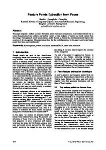
The function of the eye is to form an image; a cross-section of the eye is illustrated in Figure 1.3. Vision requires an ability to focus selectively on objects of interest. This is achieved by the ciliary muscles that hold the lens. In old age, it is these muscles which become slack and the eye loses its ability to focus at short distance. The iris, or pupil, is like an aperture on a camera and controls the amount of light entering the eye. It is a delicate system and needs protection, this is provided by the cornea (sclera). The choroid has blood vessels that supply nutrition and is opaque to cut down the amount of light. The retina is on the inside of the eye, which is where light falls to form an image. By this system, muscles rotate the eye, and shape the lens, to form an image on the fovea (focal point) where the majority of sensors are situated. The blind spot is where the optic nerve starts; there are no sensors there. Focusing involves shaping the lens, rather than positioning it as in a camera. The lens is shaped to refract close images greatly, and distant objects little, essentially by ‘stretching’ it. The distance of the focal centre of the lens varies from approximately 14 mm to around 17 mm depending on the lens shape. This implies that a world scene is translated into an area of about 2 mm2. Good vision has high acuity (sharpness), which implies that there must be very many sensors in the area where the image is formed. There are actually nearly 100 million sensors dispersed around the retina. Light falls on 4

Feature Extraction and Image Processing

Choroid

Ciliary muscle

Lens

Fovea

Blind spot Retina

Optic nerve

Figure 1.3

Human eye

these sensors to stimulate photochemical transmissions, which results in nerve impulses that are collected to form the signal transmitted by the eye. There are two types of sensor: first, the rods−these are used for black and white (scotopic) vision; and secondly, the cones–these are used for colour (photopic) vision. There are approximately 10 million cones and nearly all are found within 5° of the fovea. The remaining 100 million rods are distributed around the retina, with the majority between 20° and 5° of the fovea. Acuity is actually expressed in terms of spatial resolution (sharpness) and brightness/colour resolution, and is greatest within 1° of the fovea. There is only one type of rod, but there are three types of cones. These types are: 1. α − these sense light towards the blue end of the visual spectrum; 2. β − these sense green light; 3. γ − these sense light in the red region of the spectrum. The total response of the cones arises from summing the response of these three types of cones, this gives a response covering the whole of the visual spectrum. The rods are sensitive to light within the entire visual spectrum, and are more sensitive than the cones. Accordingly, when the light level is low, images are formed away from the fovea, to use the superior sensitivity of the rods, but without the colour vision of the cones. Note that there are actually very few of the α cones, and there are many more β and γ cones. But we can still see a lot of blue (especially given ubiquitous denim!). So, somehow, the human vision system compensates for the lack of blue sensors, to enable us to perceive it. The world would be a funny place with red water! The vision response is actually logarithmic and depends on brightness adaption from dark conditions where the image is formed on the rods, to brighter conditions where images are formed on the cones. One inherent property of the eye, known as Mach bands, affects the way we perceive Introduction

5

images. These are illustrated in Figure 1.4 and are the darker bands that appear to be where two stripes of constant shade join. By assigning values to the image brightness levels, the cross-section of plotted brightness is shown in Figure 1.4(a). This shows that the picture is formed from stripes of constant brightness. Human vision perceives an image for which the cross-section is as plotted in Figure 1.4(c). These Mach bands do not really exist, but are introduced by your eye. The bands arise from overshoot in the eyes’ response at boundaries of regions of different intensity (this aids us to differentiate between objects in our field of view). The real cross-section is illustrated in Figure 1.4(b). Note also that a human eye can distinguish only relatively few grey levels. It actually has a capability to discriminate between 32 levels (equivalent to five bits) whereas the image of Figure 1.4(a) could have many more brightness levels. This is why your perception finds it more difficult to discriminate between the low intensity bands on the left of Figure 1.4(a). (Note that that Mach bands cannot be seen in the earlier image of circles, Figure 1.2(a), due to the arrangement of grey levels.) This is the limit of our studies of the first level of human vision; for those who are interested, Cornsweet (1970) provides many more details concerning visual perception.

(a) Image showing the Mach band effect

200

200

mach0,x 100

seenx 100

0

50

100

x (b) Cross-section through (a)

Figure 1.4

0

50

100

x (c) Perceived cross-section through (a)

Illustrating the Mach band effect

So we have already identified two properties associated with the eye that it would be difficult to include, and would often be unwanted, in a computer vision system: Mach 6

Feature Extraction and Image Processing

bands and sensitivity to unsensed phenomena. These properties are integral to human vision. At present, human vision is far more sophisticated than we can hope to achieve with a computer vision system. Infrared guided-missile vision systems can actually have difficulty in distinguishing between a bird at 100 m and a plane at 10 km. Poor birds! (Lucky plane?) Human vision can handle this with ease. 1.3.2

The neural system

Neural signals provided by the eye are essentially the transformed response of the wavelength dependent receptors, the cones and the rods. One model is to combine these transformed signals by addition, as illustrated in Figure 1.5. The response is transformed by a logarithmic function, mirroring the known response of the eye. This is then multiplied by a weighting factor that controls the contribution of a particular sensor. This can be arranged to allow a combination of responses from a particular region. The weighting factors can be chosen to afford particular filtering properties. For example, in lateral inhibition, the weights for the centre sensors are much greater than the weights for those at the extreme. This allows the response of the centre sensors to dominate the combined response given by addition. If the weights in one half are chosen to be negative, whilst those in the other half are positive, then the output will show detection of contrast (change in brightness), given by the differencing action of the weighting functions.

Logarithmic response

Weighting functions

Sensor inputs

p1

log(p1)

w1 × log(p1)

p2

log(p2)

w2 × log(p2)

p3

log(p 3)

w3 × log(p3)

p4

log(p4)

w4 × log(p4)

p5

log(p5)

w5 × log(p5)

Figure 1.5

∑

Output

Neural processing

The signals from the cones can be combined in a manner that reflects chrominance (colour) and luminance (brightness). This can be achieved by subtraction of logarithmic functions, which is then equivalent to taking the logarithm of their ratio. This allows measures of chrominance to be obtained. In this manner, the signals derived from the Introduction

7

sensors are combined prior to transmission through the optic nerve. This is an experimental model, since there are many ways possible to combine the different signals together. For further information on retinal neural networks, see Ratliff (1965); an alternative study of neural processing can be found in Overington (1992). 1.3.3

Processing

The neural signals are then transmitted to two areas of the brain for further processing. These areas are the associative cortex, where links between objects are made, and the occipital cortex, where patterns are processed. It is naturally difficult to determine precisely what happens in this region of the brain. To date, there have been no volunteers for detailed study of their brain’s function (though progress with new imaging modalities such as Positive Emission Tomography or Electrical Impedance Tomography will doubtless help). For this reason, there are only psychological models to suggest how this region of the brain operates. It is well known that one function of the eye is to use edges, or boundaries, of objects. We can easily read the word in Figure 1.6(a), this is achieved by filling in the missing boundaries in the knowledge that the pattern most likely represents a printed word. But we can infer more about this image; there is a suggestion of illumination, causing shadows to appear in unlit areas. If the light source is bright, then the image will be washed out, causing the disappearance of the boundaries which are interpolated by our eyes. So there is more than just physical response, there is also knowledge, including prior knowledge of solid geometry. This situation is illustrated in Figure 1.6(b) that could represent three ‘Pacmen’ about to collide, or a white triangle placed on top of three black circles. Either situation is possible.

(a) Word?

Figure 1.6

(b) Pacmen?

How human vision uses edges

It is also possible to deceive the eye, primarily by imposing a scene that it has not been trained to handle. In the famous Zollner illusion, Figure 1.7(a), the bars appear to be slanted, whereas in reality they are vertical (check this by placing a pen between the lines): the small crossbars mislead your eye into perceiving the vertical bars as slanting. In the Ebbinghaus illusion, Figure 1.7(b), the inner circle appears to be larger when surrounded by small circles, than it appears when surrounded by larger circles. 8

Feature Extraction and Image Processing

(a) Zollner

Figure 1.7

(b) Ebbinghaus

Static illusions

There are dynamic illusions too: you can always impress children with the ‘see my wobbly pencil’ trick. Just hold the pencil loosely between your fingers then, to whoops of childish glee, when the pencil is shaken up and down, the solid pencil will appear to bend. Benham’s disk, Figure 1.8, shows how hard it is to model vision accurately. If you make up a version of this disk into a spinner (push a matchstick through the centre) and spin it anti-clockwise, you do not see three dark rings, you will see three coloured ones. The outside one will appear to be red, the middle one a sort of green, and the inner one will appear deep blue. (This can depend greatly on lighting – and contrast between the black and white on the disk. If the colours are not clear, try it in a different place, with different lighting.) You can appear to explain this when you notice that the red colours are associated with the long lines, and the blue with short lines. But this is from physics, not psychology. Now spin the disk clockwise. The order of the colours reverses: red is associated with the short lines (inside), and blue with the long lines (outside). So the argument from physics is clearly incorrect, since red is now associated with short lines not long ones, revealing the need for psychological explanation of the eyes’ function. This is not colour perception, see Armstrong (1991) for an interesting (and interactive!) study of colour theory and perception.

Figure 1.8

Benham’s disk

Naturally, there are many texts on human vision. Marr’s seminal text (Marr, 1982) is a computational investigation into human vision and visual perception, investigating it from Introduction

9

a computer vision viewpoint. For further details on pattern processing in human vision, see Bruce (1990); for more illusions see Rosenfeld (1982). One text (Kaiser, 1999) is available on line (http://www.yorku.ca/eye/thejoy.htm) which is extremely convenient. Many of the properties of human vision are hard to include in a computer vision system, but let us now look at the basic components that are used to make computers see.

1.4

Computer vision systems

Given the progress in computer technology, computer vision hardware is now relatively inexpensive; a basic computer vision system requires a camera, a camera interface and a computer. These days, some personal computers offer the capability for a basic vision system, by including a camera and its interface within the system. There are specialised systems for vision, offering high performance in more than one aspect. These can be expensive, as any specialist system is. 1.4.1

Cameras

A camera is the basic sensing element. In simple terms, most cameras rely on the property of light to cause hole/electron pairs (the charge carriers in electronics) in a conducting material. When a potential is applied (to attract the charge carriers), this charge can be sensed as current. By Ohm’s law, the voltage across a resistance is proportional to the current through it, so the current can be turned into a voltage by passing it through a resistor. The number of hole/electron pairs is proportional to the amount of incident light. Accordingly, greater charge (and hence greater voltage and current) is caused by an increase in brightness. In this manner cameras can provide as output, a voltage which is proportional to the brightness of the points imaged by the camera. Cameras are usually arranged to supply video according to a specified standard. Most will aim to satisfy the CCIR standard that exists for closed circuit television systems. There are three main types of camera: vidicons, charge coupled devices (CCDs) and, more recently, CMOS cameras (Complementary Metal Oxide Silicon – now the dominant technology for logic circuit implementation). Vidicons are the older (analogue) technology, which though cheap (mainly by virtue of longevity in production) are now being replaced by the newer CCD and CMOS digital technologies. The digital technologies, currently CCDs, now dominate much of the camera market because they are lightweight and cheap (with other advantages) and are therefore used in the domestic video market. Vidicons operate in a manner akin to a television in reverse. The image is formed on a screen, and then sensed by an electron beam that is scanned across the screen. This produces an output which is continuous, the output voltage is proportional to the brightness of points in the scanned line, and is a continuous signal, a voltage which varies continuously with time. On the other hand, CCDs and CMOS cameras use an array of sensors; these are regions where charge is collected which is proportional to the light incident on that region. This is then available in discrete, or sampled, form as opposed to the continuous sensing of a vidicon. This is similar to human vision with its array of cones and rods, but digital cameras use a rectangular regularly spaced lattice whereas human vision uses a hexagonal lattice with irregular spacing. Two main types of semiconductor pixel sensors are illustrated in Figure 1.9. In the passive sensor, the charge generated by incident light is presented to a bus through a pass 10

Feature Extraction and Image Processing

transistor. When the signal Tx is activated, the pass transistor is enabled and the sensor provides a capacitance to the bus, one that is proportional to the incident light. An active pixel includes an amplifier circuit that can compensate for limited fill factor of the photodiode. The select signal again controls presentation of the sensor’s information to the bus. A further reset signal allows the charge site to be cleared when the image is rescanned.

VDD

Tx Reset

Incident light

Incident light

Column bus

Select

Column bus (a) Passive

Figure 1.9

(b) Active

Pixel sensors

The basis of a CCD sensor is illustrated in Figure 1.10. The number of charge sites gives the resolution of the CCD sensor; the contents of the charge sites (or buckets) need to be converted to an output (voltage) signal. In simple terms, the contents of the buckets are emptied into vertical transport registers which are shift registers moving information towards

Vertical transport register

Vertical transport register

Vertical transport register

Horizontal transport register Signal conditioning

Video output

Control

Control inputs

Pixel sensors

Figure 1.10

CCD sensing element

Introduction

11

the horizontal transport registers. This is the column bus supplied by the pixel sensors. The horizontal transport registers empty the information row by row (point by point) into a signal conditioning unit which transforms the sensed charge into a voltage which is proportional to the charge in a bucket, and hence proportional to the brightness of the corresponding point in the scene imaged by the camera. CMOS cameras are like a form of memory: the charge incident on a particular site in a two-dimensional lattice is proportional to the brightness at a point. The charge is then read like computer memory. (In fact, a computer memory RAM chip can act as a rudimentary form of camera when the circuit – the one buried in the chip – is exposed to light.) There are many more varieties of vidicon (Chalnicon etc.) than there are of CCD technology (Charge Injection Device etc.), perhaps due to the greater age of basic vidicon technology. Vidicons were cheap but had a number of intrinsic performance problems. The scanning process essentially relied on ‘moving parts’. As such, the camera performance changed with time, as parts wore; this is known as ageing. Also, it is possible to burn an image into the scanned screen by using high incident light levels; vidicons also suffered lag that is a delay in response to moving objects in a scene. On the other hand, the digital technologies are dependent on the physical arrangement of charge sites and as such do not suffer from ageing, but can suffer from irregularity in the charge sites’ (silicon) material. The underlying technology also makes CCD and CMOS cameras less sensitive to lag and burn, but the signals associated with the CCD transport registers can give rise to readout effects. CCDs actually only came to dominate camera technology when technological difficulty associated with quantum efficiency (the magnitude of response to incident light) for the shorter, blue, wavelengths was solved. One of the major problems in CCD cameras is blooming, where bright (incident) light causes a bright spot to grow and disperse in the image (this used to happen in the analogue technologies too). This happens much less in CMOS cameras because the charge sites can be much better defined and reading their data is equivalent to reading memory sites as opposed to shuffling charge between sites. Also, CMOS cameras have now overcome the problem of fixed pattern noise that plagued earlier MOS cameras. CMOS cameras are actually much more recent than CCDs. This begs a question as to which is best: CMOS or CCD? Given that they will both be subject to much continued development though CMOS is a cheaper technology and because it lends itself directly to intelligent cameras with on-board processing. This is mainly because the feature size of points (pixels) in a CCD sensor is limited to about 4 µm so that enough light is collected. In contrast, the feature size in CMOS technology is considerably smaller, currently at around 0.1 µm. Accordingly, it is now possible to integrate signal processing within the camera chip and thus it is perhaps possible that CMOS cameras will eventually replace CCD technologies for many applications. However, the more modern CCDs also have on-board circuitry, and their process technology is more mature, so the debate will continue! Finally, there are specialist cameras, which include high-resolution devices (which can give pictures with a great number of points), low-light level cameras which can operate in very dark conditions (this is where vidicon technology is still found) and infrared cameras which sense heat to provide thermal images. For more detail concerning camera practicalities and imaging systems see, for example, Awcock and Thomas (1995) or Davies (1994). For practical minutiae on cameras, and on video in general, Lenk’s Video Handbook (Lenk, 1991) has a wealth of detail. For more detail on sensor development, particularly CMOS, the article (Fossum, 1997) is well worth a look.

12

Feature Extraction and Image Processing

1.4.2

Computer interfaces

The basic computer interface needs to convert an analogue signal from a camera into a set of digital numbers. The interface system is called a framegrabber since it grabs frames of data from a video sequence, and is illustrated in Figure 1.11. Note that intelligent cameras which provide digital information do not need this particular interface, just one which allows storage of their data. However, a conventional camera signal is continuous and is transformed into digital (discrete) format using an Analogue to Digital (A/D) converter. Flash converters are usually used due to the high speed required for conversion (say 11 MHz that cannot be met by any other conversion technology). The video signal requires conditioning prior to conversion; this includes DC restoration to ensure that the correct DC level is attributed to the incoming video signal. Usually, 8-bit A/D converters are used; at 6 dB/bit, this gives 48 dB which just satisfies the CCIR stated bandwidth of approximately 45 dB. The output of the A/D converter is often fed to look-up tables (LUTs) which implement designated conversion of the input data, but in hardware, rather than in software, and this is very fast. The outputs of the A/D converter are then stored in computer memory. This is now often arranged to be dual-ported memory that is shared by the computer and the framegrabber (as such the framestore is memory-mapped): the framegrabber only takes control of the image memory when it is acquiring, and storing, an image. Alternative approaches can use Dynamic Memory Access (DMA) or, even, external memory, but computer memory is now so cheap that such design techniques are rarely used.

Input video

Signal conditioning

A/D converter

Control

Look-up table

Image memory

Computer interface

Computer

Figure 1.11

A computer interface – the framegrabber

There are clearly many different ways to design framegrabber units, especially for specialist systems. Note that the control circuitry has to determine exactly when image data is to be sampled. This is controlled by synchronisation pulses that are supplied within the video signal and can be extracted by a circuit known as a sync stripper (essentially a high gain amplifier). The sync signals actually control the way video information is constructed. Television pictures are constructed from a set of lines, those lines scanned by a camera. In order to reduce requirements on transmission (and for viewing), the 625 lines (in the PAL system) are transmitted in two fields, each of 312.5 lines, as illustrated in Figure 1.12. (There was a big debate between the computer producers who don’t want interlacing, and the television broadcasters who do.) If you look at a television, but not directly, the flicker due to interlacing can be perceived. When you look at the television directly, persistence in the human eye ensures that you do not see the flicker. These fields are called the odd and Introduction

13

even fields. There is also an aspect ratio in picture transmission: pictures are arranged to be 1.33 times longer than they are high. These factors are chosen to make television images attractive to human vision, and can complicate the design of a framegrabber unit. Nowadays, digital video cameras can provide the digital output, in progressive scan (without interlacing). Life just gets easier!

Aspect ratio 4 3

Television picture

Even field lines

Figure 1.12

Odd field lines

Interlacing in television pictures

This completes the material we need to cover for basic computer vision systems. For more detail concerning practicalities of computer vision systems see, for example, Davies (1994) and Baxes (1994). 1.4.3

Processing an image

Most image processing and computer vision techniques are implemented in computer software. Often, only the simplest techniques migrate to hardware; though coding techniques to maximise efficiency in image transmission are of sufficient commercial interest that they have warranted extensive, and very sophisticated, hardware development. The systems include the Joint Photographic Expert Group (JPEG) and the Moving Picture Expert Group (MPEG) image coding formats. C and C++ are by now the most popular languages for vision system implementation: C because of its strengths in integrating high- and low-level functions, and the availability of good compilers. As systems become more complex, C++ becomes more attractive when encapsulation and polymorphism may be exploited. Many people now use Java as a development language partly due to platform independence, but also due to ease in implementation (though some claim that speed/efficiency is not as good as in C/C++). There is considerable implementation advantage associated with use of the JavaTM Advanced Imaging API (Application Programming Interface). There are some textbooks that offer image processing systems implemented in these languages. Also, there are many commercial packages available, though these are often limited to basic techniques, and do not include the more sophisticated shape extraction techniques. The Khoros image processing system has attracted much interest; this is a schematic (data-flow) image processing system where a user links together chosen modules. This allows for better visualisation of 14

Feature Extraction and Image Processing

information flow during processing. However, the underlying mathematics is not made clear to the user, as it can be when a mathematical system is used. There is a new textbook, and a very readable one at that, by Nick Efford (Efford, 2000) which is based entirely on Java and includes, via a CD, the classes necessary for image processing software development. A set of WWW links are shown in Table 1.2 for established freeware and commercial software image processing systems. What is perhaps the best selection can be found at the general site, from the computer vision homepage software site (repeated later in Table 1.5). Table 1.2

Software package websites

Packages (freeware or student version indicated by *) General Site

Carnegie Mellon

http://www.cs.cmu.edu/afs/cs/ project/cil/ftp/html/v-source.html

Khoros

Khoral Research Hannover U

http://www.khoral.com/ http://www.tnt.uni-hannover.de/ soft/imgproc/khoros/

AdOculos* (+ Textbook)

The Imaging Source

http://www.theimagingsource.com/ catalog/soft/dbs/ao.htm

CVIPtools* LaboImage*

Southern Illinois U Geneva U

http://www.ee.siue.edu/CVIPtools/ http://cuiwww.unige.ch/~vision/ LaboImage/labo.html

TN-Image*

Thomas J. Nelson

http://las1.ninds.nih.gov/tnimagemanual/tnimage-manual.html

1.5

Mathematical systems

In recent years, a number of mathematical systems have been developed. These offer what is virtually a word-processing system for mathematicians and many are screen-based using a Windows system. The advantage of these systems is that you can transpose mathematics pretty well directly from textbooks, and see how it works. Code functionality is not obscured by the use of data structures, though this can make the code appear cumbersome. A major advantage is that the system provides the low-level functionality and data visualisation schemes, allowing the user to concentrate on techniques alone. Accordingly, these systems afford an excellent route to understand, and appreciate, mathematical systems prior to development of application code, and to check the final code functions correctly. 1.5.1

Mathematical tools

Mathcad, Mathematica, Maple and Matlab are amongst the most popular of current tools. There have been surveys that compare their efficacy, but it is difficult to ensure precise comparison due to the impressive speed of development of techniques. Most systems have their protagonists and detractors, as in any commercial system. There are many books which use these packages for particular subjects, and there are often handbooks as addenda to the packages. We shall use both Matlab and Mathcad throughout this text as they are Introduction

15

perhaps the two most popular of the mathematical systems. We shall describe Matlab later, as it is different from Mathcad, though the aim is the same. The website links for the main mathematical packages are given in Table 1.3.

Table 1.3

Mathematical package websites

General Math-Net Links to the Mathematical World

Math-Net (Germany)

http://www.math-net.de/

Mathcad

MathSoft

http://www.mathcad.com/

Mathematica

Wolfram Research

http://www.wri.com/

Matlab

Mathworks

http://www.mathworks.com/

Vendors

1.5.2

Hello Mathcad, Hello images!

The current state of evolution is Mathcad 2001; this adds much to version 6 which was where the system became useful as it included a programming language for the first time. Mathcad offers a compromise between many performance factors, and is available at low cost. If you do not want to buy it, there was a free worksheet viewer called Mathcad Explorer which operates in read-only mode. There is an image processing handbook available with Mathcad, but it does not include many of the more sophisticated feature extraction techniques. Mathcad uses worksheets to implement mathematical analysis. The flow of calculation is very similar to using a piece of paper: calculation starts at the top of a document, and flows left-to-right and downward. Data is available to later calculation (and to calculation to the right), but is not available to prior calculation, much as is the case when calculation is written manually on paper. Mathcad uses the Maple mathematical library to extend its functionality. To ensure that equations can migrate easily from a textbook to application, Mathcad uses a WYSIWYG (What You See Is What You Get) notation (its equation editor is actually not dissimilar to the Microsoft Equation (Word) editor). Images are actually spatial data, data which is indexed by two spatial co-ordinates. The camera senses the brightness at a point with co-ordinates x, y. Usually, x and y refer to the horizontal and vertical axes, respectively. Throughout this text we shall work in orthographic projection, ignoring perspective, where real world co-ordinates map directly to x and y coordinates in an image. The homogeneous co-ordinate system is a popular and proven method for handling three-dimensional co-ordinate systems (x, y and z where z is depth). Since it is not used directly in the text, it is included as Appendix 1 (Section 9.1). The brightness sensed by the camera is transformed to a signal which is then fed to the A/D converter and stored as a value within the computer, referenced to the co-ordinates x, y in the image. Accordingly, a computer image is a matrix of points. For a greyscale image, the value of each point is proportional to the brightness of the corresponding point in the scene viewed, and imaged, by the camera. These points are the picture elements, or pixels. 16

Feature Extraction and Image Processing

Consider, for example, the matrix of pixel values in Figure 1.13(a). This can be viewed as a surface (or function) in Figure 1.13(b), or as an image in Figure 1.13(c). In Figure 1.13(c) the brightness of each point is proportional to the value of its pixel. This gives the synthesised image of a bright square on a dark background. The square is bright where the pixels have a value around 40 brightness levels; the background is dark, these pixels have a value near 0 brightness levels. This image is first given a label, pic, and then pic is allocated, :=, to the matrix defined by using the matrix dialog box in Mathcad, specifying a matrix with 8 rows and 8 columns. The pixel values are then entered one by one until the matrix is complete (alternatively, the matrix can be specified by using a subroutine, but that comes later). Note that neither the background, nor the square, has a constant brightness. This is because noise has been added to the image. If we want to evaluate the performance of a computer vision technique on an image, but without the noise, we can simply remove it (one of the advantages to using synthetic images). The matrix becomes an image when it is viewed as a picture, as in Figure 1.13(c). This is done either by presenting it as a surface plot, rotated by zero degrees and viewed from above, or by using Mathcad’s picture facility. As a surface plot, Mathcad allows the user to select a greyscale image, and the patch plot option allows an image to be presented as point values.

1 2  3  4 pic : =  1  2  1  1

2 2 1 1 2 1 2 2

3 3 38 45 43 39 1 1

4 2 39 44 44 41 2 3

1 1 37 41 40 42 2 1

(a) Matrix

Figure 1.13

1 2 36 42 39 40 3 1

2 2 3 2 1 2 1 4

1 1 1  1 3  1  1 2

40 30 20 10 0 2 4 6

6

pic (b) Surface plot

(c) Image

Synthesised image of a square

Mathcad stores matrices in row-column format. The co-ordinate system used throughout this text has x as the horizontal axis and y as the vertical axis (as conventional). Accordingly, x is the column count and y is the row count so a point (in Mathcad) at co-ordinates x,y is actually accessed as picy,x. The origin is at co-ordinates x = 0 and y = 0 so pic0,0 is the magnitude of the point at the origin and pic2,2 is the point at the third row and third column and pic3,2 is the point at the third column and fourth row, as shown in Code 1.1 (the points can be seen in Figure 1.13(a)). Since the origin is at (0,0) the bottom right-hand point, at the last column and row, has co-ordinates (7,7). The number of rows and the number of columns in a matrix, the dimensions of an image, can be obtained by using the Mathcad rows and cols functions, respectively, and again in Code 1.1. pic2,2=38 pic3,2=45 rows(pic)=8 cols(pic)=8 Code 1.1

Accessing an image in Mathcad

Introduction

17

This synthetic image can be processed using the Mathcad programming language, which can be invoked by selecting the appropriate dialog box. This allows for conventional for, while and if statements, and the earlier assignment operator which is := in non-code sections is replaced by ← in sections of code. A subroutine that inverts the brightness level at each point, by subtracting it from the maximum brightness level in the original image, is illustrated in Code 1.2. This uses for loops to index the rows and the columns, and then calculates a new pixel value by subtracting the value at that point from the maximum obtained by Mathcad’s max function. When the whole image has been processed, the new picture is returned to be assigned to the label newpic. The resulting matrix is shown in Figure 1.14(a). When this is viewed as a surface, Figure 1.14(b), the inverted brightness levels mean that the square appears dark and its surroundings appear white, as in Figure 1.14(c).

New_pic:= for x∈0..cols(pic)–1 for y∈0..rows(pic)–1 newpicturey,x ←max(pic)–picy,x newpicture Code 1.2

Processing image points in Mathcad

 44  43   42   41 new_pic =  44   43   44  44

43 43 44 44 43 44 43 43

42 42 7 0 2 6 44 44

41 43 6 1 1 4 43 42

(a) Matrix

Figure 1.14

44 44 8 4 5 3 43 44

44 43 9 3 6 5 42 44

43 43 42 43 44 43 44 41

44  44  44   44  42   44   44  43 

4 6

40 30 20 10 0 2

new_pic (b) Surface plot

6

(c) Image

Image of a square after inversion

Routines can be formulated as functions, so they can be invoked to process a chosen picture, rather than restricted to a specific image. Mathcad functions are conventional, we simply add two arguments (one is the image to be processed, the other is the brightness to be added), and use the arguments as local variables, to give the add function illustrated in Code 1.3. To add a value, we simply call the function and supply an image and the chosen brightness level as the arguments. add_value(inpic,value):= for x 0..cols(inpic)–1 for y 0..rows(inpic)–1 newpicturey,x ←inpicy,x+value newpicture Code 1.3

18

Function to add a value to an image in Mathcad

Feature Extraction and Image Processing

Mathematically, for an image which is a matrix of N × N points, the brightness of the pixels in a new picture (matrix), N, is the result of adding b brightness values to the pixels in the old picture, O, given by: Nx,y = Ox,y + b

∀ x, y ∈ 1, N

(1.1)

Real images naturally have many points. Unfortunately, the Mathcad matrix dialog box only allows matrices that are 10 rows and 10 columns at most, i.e. a 10 × 10 matrix. Real images can be 512 × 512, but are often 256 × 256 or 128 × 128, this implies a storage requirement for 262 144, 65 536 and 16 384 pixels, respectively. Since Mathcad stores all points as high precision, complex floating point numbers, 512 × 512 images require too much storage, but 256 × 256 and 128 × 128 images can be handled with ease. Since this cannot be achieved by the dialog box, Mathcad has to be ‘tricked’ into accepting an image of this size. Figure 1.15 shows the image of a human face captured by a camera. This image has been stored in Windows bitmap (.BMP) format. This can be read into a Mathcad worksheet using the READBMP command (yes, capitals please! – Mathcad can’t handle readbmp), and is assigned to a variable. It is inadvisable to attempt to display this using the Mathcad surface plot facility as it can be slow for images, and require a lot of memory.

0 1 2 0 78 75 73 1 74 71 74 2 70 73 79 3 70 77 83 4 74 77 79 Face = 5 76 77 78 6 75 79 78 7 76 77 70 8 75 76 61 9 77 76 55 10 77 70 45 11 73 60 37 12 71 53 34

3 4 79 83 77 79 77 74 77 66 70 53 64 45 60 43 48 36 40 33 34 27 27 19 26 18 26 18

5 6 77 73 71 66 64 55 52 42 37 29 30 22 28 16 24 12 21 12 16 9 9 7 5 7 6 7

7 79 71 55 47 37 26 20 21 24 21 26 32 33

8 9 79 77 74 79 66 78 63 74 53 68 45 66 48 71 51 73 55 79 56 84 61 88 68 88 67 88

10 11 79 78 79 77 77 81 75 80 77 78 80 86 81 91 84 91 88 91 93 95 97 97 95 99 96 103

(a) Part of original image as a matrix

(c) Bitmap of original image

Figure 1.15

0 1 2 3 4 New face = 5 6

0 1 158 155 154 151 150 153 150 157 154 157 156 157 155 159

2 3 153 159 154 157 159 157 163 157 159 150 158 144 158 140

4 163 159 154 146 133 125 123

5 6 157 153 151 146 144 135 132 122 117 109 110 102 108 96

7 8 159 159 151 154 135 146 127 143 117 133 106 125 100 128

7 8 9 10 11 12

156 157 155 156 157 156 157 150 153 140 151 133

150 128 141 120 135 114 125 107 117 106 114 106

116 113 107 90 98 98

104 101 96 89 85 86

101 131 104 135 101 136 106 141 112 148 113 147

92 92 89 87 87 87

(b) Part of processed image as a matrix

(d) Bitmap of processed image

Processing an image of a face

Introduction

19

It is best to view an image using Mathcad’s picture facility or to store it using the WRITEBMP command, and then look at it using a bitmap viewer. So if we are to make the image of the face brighter, by addition, by the routine in Code 1.3, via the code in Code 1.4, the result is as shown in Figure 1.15. The matrix listings in Figure 1.15(a) and Figure 1.15(b) show that 80 has been added to each point (these only show the top left-hand section of the image where the bright points relate to the blonde hair, the dark points are the gap between the hair and the face). The effect will be to make each point appear brighter as seen by comparison of the (darker) original image, Figure 1.15(c), with the (brighter) result of addition, Figure 1.15(d). In Chapter 3 we will investigate techniques which can be used to manipulate the image brightness to show the face in a much better way. For the moment though, we are just seeing how Mathcad can be used, in a simple way, to process pictures. face :=READBMP(rhdark) newface :=add_value(face,80) WRITEBMP(rhligh) :=newface Code 1.4

Processing an image

Naturally, Mathcad was used to generate the image used to demonstrate the Mach band effect; the code is given in Code 1.5. First, an image is defined by copying the face image (from Code 1.4) to an image labelled mach. Then, the floor function (which returns the nearest integer less than its argument) is used to create the bands, scaled by an amount appropriate to introduce sufficient contrast (the division by 21.5 gives six bands in the image of Figure 1.4(a)). The cross-section and the perceived cross-section of the image were both generated by Mathcad’s X-Y plot facility, using appropriate code for the perceived cross-section. mach := face mach := for x∈0..cols(mach)–1 for y∈0..rows(mach)–1   machy,x←40·floor  x   21.5 

mach Code 1.5

Creating the Image of Figure 1.4(a)

The translation of the Mathcad code into application can be rather prolix when compared with the Mathcad version by the necessity to include low-level functions. Since these can obscure the basic image processing functionality, Mathcad is used throughout this book to show you how the techniques work. The translation to application code is perhaps easier via Matlab (it offers direct compilation of the code). There is also an electronic version of this book which is a collection of worksheets to help you learn the subject; and an example Mathcad worksheet is given in Appendix 3 (Section 9.3). You can download these worksheets from this book’s website (http://www.ecs.soton.ac.uk/~msn/book/) and there is a link to Mathcad Explorer there too. You can then use the algorithms as a basis for developing your own application code. This provides a good way to verify that your code 20

Feature Extraction and Image Processing

actually works: you can compare the results of your final application code with those of the original mathematical description. If your final application code and the Mathcad implementation are both correct, the results should be the same. Naturally, your application code will be much faster than in Mathcad, and will benefit from the GUI you’ve developed. 1.5.3

Hello Matlab!

Matlab is rather different from Mathcad. It is not a WYSIWYG system but instead it is more screen-based. It was originally developed for matrix functions, hence the ‘Mat’ in the name. Like Mathcad, it offers a set of mathematical tools and visualisation capabilities in a manner arranged to be very similar to conventional computer programs. In some users’ views, a WYSIWYG system like Mathcad is easier to start with but there are a number of advantages to Matlab, not least the potential speed advantage in computation and the facility for debugging, together with a considerable amount of established support. Again, there is an image processing toolkit supporting Matlab, but it is rather limited compared with the range of techniques exposed in this text. The current version is Matlab 5.3.1, but these systems evolve fast! Essentially, Matlab is the set of instructions that process the data stored in a workspace, which can be extended by user-written commands. The workspace stores the different lists of data and these data can be stored in a MAT file; the user-written commands are functions that are stored in M-files (files with extension .M). The procedure operates by instructions at the command line to process the workspace data using either one of Matlab’s own commands, or using your own commands. The results can be visualised as graphs, surfaces or as images, as in Mathcad. The system runs on Unix/Linux or Windows and on Macintosh systems. A student version is available at low cost. There is no viewer available for Matlab, you have to have access to a system for which it is installed. As the system is not based around worksheets, we shall use a script which is the simplest type of M-file, as illustrated in Code 1.6. To start the Matlab system, type MATLAB at the command line. At the Matlab prompt (>>) type chapter1 to load and run the script (given that the file chapter1.m is saved in the directory you are working in). Here, we can see that there are no text boxes and so comments are preceded by a %. The first command is one that allocates data to our variable pic. There is a more sophisticated way to input this in the Matlab system, but that is not available here. The points are addressed in row-column format and the origin is at coordinates y = 1 and x = 1. So we then access these point pic3,3 as the third column of the third row and pic4,3 is the point in the third column of the fourth row. Having set the display facility to black and white, we can view the array pic as a surface. When the surface, illustrated in Figure 1.16(a), is plotted, then Matlab has been made to pause until you press Return before moving on. Here, when you press Return, you will next see the image of the array, Figure 1.16(b). We can use Matlab’s own command to interrogate the data: these commands find use in the M-files that store subroutines. An example routine is called after this. This subroutine is stored in a file called invert.m and is a function that inverts brightness by subtracting the value of each point from the array’s maximum value. The code is illustrated in Code 1.7. Note that this code uses for loops which are best avoided to improve speed, using Matlab’s vectorised operations (as in Mathcad), but are used here to make the implementations clearer to those with a C background. The whole procedure can actually be implemented by the command inverted=max(max(pic))-pic. In fact, one of Matlab’s assets is Introduction

21

%Chapter 1 Introduction (Hello Matlab) CHAPTER1.M %Written by: Mark S. Nixon disp(‘Welcome to the Chapter1 script’) disp(‘This worksheet is the companion to Chapter 1 and is an introduction.’) disp(‘It is the source of Section 1.4.3 Hello Matlab.’) disp(‘The worksheet follows the text directly and allows you to process basic images.’) disp(‘Let us define a matrix, a synthetic computer image called pic.’) pic = [1 2 3 4 1 2 1 1

2 2 1 1 2 1 2 2

3 3 38 45 43 39 1 1

4 2 39 44 44 41 2 3

1 1 37 41 40 42 2 1

1 2 36 42 39 40 3 1

2 2 3 2 1 2 1 4

1; 1; 1; 1; 3; 1; 1; 2]

%Pixels are addressed in row-column format. %Using x for the horizontal axis(a column count), and y for the vertical axis (a row %count) then picture points are addressed as pic(y,x). The origin is at co-ordinates %(1,1), so the point pic(3,3) is on the third row and third column; the point pic(4,3) %is on the fourth row, at the third column. Let’s print them: disp (‘The element pic(3,3)is’) pic(3,3) disp(‘The element pic(4,3)is’) pic(4,3) %We’ll set the output display to black and white colormap(gray); %We can view the matrix as a surface plot disp (‘We shall now view it as a surface plot (play with the controls to see it in relief)’) disp(‘When you are ready to move on, press RETURN’) surface(pic); %Let’s hold a while so we can view it pause; %Or view it as an image disp (‘We shall now view the array as an image’) disp(‘When you are ready to move on, press RETURN) imagesc(pic); %Let’s hold a while so we can view it pause; %Let’s look at the array’s dimensions

22

Feature Extraction and Image Processing

disp(‘The dimensions of the array are’) size(pic) %now let’s invoke a routine that inverts the image inverted_pic=invert(pic); %Let’s print it out to check it disp(‘When we invert it by subtracting each point from the maximum, we get’) inverted_pic %And view it disp(‘And when viewed as an image, we see’) disp(‘When you are ready to move on, press RETURN’) imagesc(inverted_pic); %Let’s hold a while so we can view it pause; disp(‘We shall now read in a bitmap image, and view it’) disp(‘When you are ready to move on, press RETURN’) face=imread(‘rhdark.bmp’,‘bmp’); imagesc(face); pause; %Change from unsigned integer(unit8) to double precision so we can process it face=double(face); disp(‘Now we shall invert it, and view the inverted image’) inverted_face=invert(face); imagesc(inverted_face); disp(‘So we now know how to process images in Matlab. We shall be using this later!’) Code 1.6

Matlab script for chapter 1

1 50 2

40

3

30 20

4

10 5

0 8

6

6 4

7 2 0 1

2

3

4

5

6

(a) Matlab surface plot

Figure 1.16

7

8 8 1

2

3

4

5

6

7

8

(b) Matlab image

Matlab image visualisation

Introduction

23

a ‘profiler’ which allows you to determine exactly how much time is spent on different parts of your programs. Naturally, there is facility for importing graphics files, which is actually rather more extensive (i.e. it accepts a wider range of file formats) than available in Mathcad. When images are used, this reveals that unlike Mathcad which stores all variables as full precision real numbers, Matlab has a range of datatypes. We must move from the unsigned integer datatype, used for images, to the double precision datatype to allow processing as a set of real numbers. In these ways Matlab can, and will be used to process images throughout this book. As with the Mathcad worksheets, there are Matlab scripts available at the website for on-line tutorial support of the material in this book; an abbreviated example worksheet is given in Appendix 4 (Section 9.4). function inverted=invert(image) %Subtract image point brightness from maximum % % Usage: [new image]=invert(image) % % Parameters: image-array of points % % Author: Mark S. Nixon %get dimensions [rows,cols]=size(image); %find the maximum maxi=max(max(image)); %subtract image points from maximum for x=1:cols %address all columns for y=1:rows %address all rows inverted(y,x)=maxi-image(y,x); end end Code 1.7

1.6

Matlab function (invert.m) to invert an image

Associated literature

1.6.1

Journals and magazines

As in any academic subject, there are many sources of literature. The professional magazines include those that are more systems oriented, like Image Processing and Advanced Imaging. These provide more general articles, and are often a good source of information about new computer vision products. For example, Image Processing often surveys available equipment, such as cameras and monitors, and provides a tabulated listing of those available, including some of the factors by which you might choose to purchase them. Advanced Imaging is another professional journal that can cover material of commercial and academic interest. There is a wide selection of research journals – probably more than you can find in your nearest library unless it is particularly well stocked. These journals have different merits: some are targeted at short papers only, whereas some have short and long papers; some are more dedicated to the development of new theory whereas others are more pragmatic and 24

Feature Extraction and Image Processing

focus more on practical, working, image processing systems. But it is rather naive to classify journals in this way, since all journals welcome good research, with new ideas, which has been demonstrated to satisfy promising objectives. The main research journals include: IEEE Transactions on: Pattern Analysis and Machine Intelligence (in later references this will be abbreviated to IEEE Trans. on PAMI); Image Processing (IP); Systems, Man and Cybernetics (SMC); and Medical Imaging (there are many more IEEE transactions, some of which sometimes publish papers of interest in image processing and computer vision). The IEEE Transactions are usually found in (university) libraries since they are available at comparatively low cost. Computer Vision and Image Understanding and Graphical Models and Image Processing arose from the splitting of one of the subject’s earlier journals, Computer Vision, Graphics and Image Processing (CVGIP), into two parts. Do not confuse Pattern Recognition (Pattern Recog.) with Pattern Recognition Letters (Pattern Recog. Lett.), published under the aegis of the Pattern Recognition Society and the International Association of Pattern Recognition, respectively, since the latter contains shorter papers only. The International Journal of Computer Vision is a more recent journal whereas Image and Vision Computing was established in the early 1980s. Finally, do not miss out on the IEE Proceedings – Vision, Image and Signal Processing and IEE Proceedings – Digital Techniques. Some of the journals are now on-line but usually to subscribers only, in the UK through Ingenta through BIDS (you need an account at Bath Information and Data Services at http://www.bids.ac.uk/). Academic Press appear to be mostly on-line now, including Computer Vision and Image Understanding, Graphical Models and Image Processing and Real-Time Imaging at http://www.apnet.com/www/journal/iv.htm, http:/ / w w w . a p n e t . c o m / w w w / j o u r n a l / i p . h t m , and h t t p : / / w w w . academicpress.com/rti respectively. 1.6.2

Textbooks

There are many textbooks in this area. Increasingly, there are web versions, or web support, as summarised in Table 1.4. This text aims to start at the foundation of computer vision, and ends very close to a research level. Its content specifically addresses techniques for image analysis, considering shape analysis in particular. Mathcad and Matlab are used as a vehicle to demonstrate implementation, which is rarely considered in other texts. But there are other texts, and these can help you to develop your interest in other areas of computer vision. This section includes only a selection of some of the texts. There are more than these, some of which will be referred to in later chapters; each offers a particular view or insight into computer vision and image processing. The introductory texts include: Fairhurst, M. C.: Computer Vision for Robotic Systems (Fairhurst, 1988); Low, A.: Introductory Computer Vision and Image Processing (Low, 1991); Teuber, J.: Digital Image Processing (Teuber, 1993); and Baxes, G. A.: Digital Image Processing, Principles and Applications (Baxes, (1994) which includes software and good coverage of image processing hardware. Some of the main textbooks include: Marr, D.: Vision (Marr, 1982) which concerns vision and visual perception (as previously mentioned); Jain, A. K.: Fundamentals of Computer Vision (Jain, 1989) which is stacked with theory and technique, but omits implementation and some image analysis; Sonka, M., Hllavac, V. and Boyle, R. Image Processing, Analysis and Computer Vision (Sonka, 1998) offers more modern coverage of computer vision including many more recent techniques, together with pseudocode Introduction

25

Table 1.4

Web textbooks and homepages

This book’s homepage

Southampton U

http://www.ecs.soton.ac.uk/~msn/book/

CVOnline

Edinburgh U

http://www.dai.ed.ac.uk/CVonline/

Ad Oculos

Imaging Source

http://www.theimagingsource. com/prod/link/adoculos.htm

Image Processing Fundamentals

Delft University

http://www.ph.tn.tudelft.nl/ Courses/FIP/noframes/fip.html

World of Mathematics

Wolfram Research

http://mathworld.wolfram.com

Numerical Recipes Cambridge University Press

http://www.nr.com/

The Joy of Visual Perception

York U

http://www.yorku.ca/research/ vision/eye/thejoy.htm

Machine Vision homepage

Penn State

http://vision.cse.psu.edu/

Active Contours homepage

Oxford U

http://www.robots.ox.ac. uk/~contours/

implementation but omitting some image processing theory; Jain, R. C., Kasturi, R. and Schunk, B. G.: Machine Vision (Jain, 1995) offers concise and modern coverage of 3D and motion (there is an on-line website at http://vision.cse.psu.edu/ with code and images, together with corrections); Gonzalez, R. C. and Wintz, P.: Digital Image Processing (Gonzalez, 1987) has more tutorial element than many of the basically theoretical texts; Rosenfeld, A. and Kak, A. C.: Digital Picture Processing (Rosenfeld and Kak, 1982) is rather dated now, but is a well-proven text for much of the basic material; and Pratt, W. K.: Digital Image Processing (Pratt, 1992) which was originally one of the earliest books on image processing and, like Rosenfeld and Kak, is a well-proven text for much of the basic material, particularly image transforms. Despite its name, the recent text called Active Contours (Blake, 1998) concentrates rather more on models of motion and deformation and probabalistic treatment of shape and motion, than on the active contours which we shall find here. As such it is a more research text, reviewing many of the advanced techniques to describe shapes and their motion. A recent text in this field, Image Processing – The Fundamentals (Petrou, 1999) surveys the subject (as its title implies) from an image processing viewpoint covering not only image transforms, but also restoration and enhancement before edge detection. The latter of these is most appropriate for one of the major contributors to that subject. Also, Kasturi, R. and Jain, R. C. (eds): Computer Vision: Principles (Kasturi, 1991a) and Computer Vision: Advances and Applications (Kasturi, 1991b) presents a collection of seminal papers in computer vision, many of which are cited in their original form (rather than in this volume) in later chapters. There are other interesting edited collections (Chellappa, 1992), one edition (Bowyer, 1996) honours Azriel Rosenfeld’s many contributions. Books which include a software implementation include: Lindley, C. A.: Practical Image Processing in C (Lindley, 1991) and Pitas, I.: Digital Image Processing Algorithms (Pitas, 1993) which both cover basic image processing and computer vision algorithms. 26

Feature Extraction and Image Processing

Parker, J. R.: Practical Computer Vision Using C (Parker, 1994) offers an excellent description and implementation of low-level image processing tasks within a well-developed framework, but again does not extend to some of the more recent and higher level processes in computer vision and includes little theory though there is more in his later text Image Processing and Computer Vision (Parker, 1996). A recent text Computer Vision and Image Processing (Umbaugh, 1998) takes an applications-oriented approach to computer vision and image processing, offering a variety of techniques in an engineering format, together with a working package with a GUI. One recent text concentrates on Java only, Image Processing in Java (Lyon, 1999), and concentrates more on image processing systems implementation than on feature extraction (giving basic methods only). As already mentioned, the newest textbook (Efford, 2000) offers Java implementation, though it omits much of the mathematical detail making it a lighter (more enjoyable?) read. Masters, T.: Signal and Image Processing with Neural Networks – A C++ Sourcebook (Masters, 1994) offers good guidance in combining image processing technique with neural networks and gives code for basic image processing technique, such as frequency domain transformation. There are now a number of books on the web as given in Table 1.4. This book’s homepage has a link to these web-based texts, and will be kept as up to date as possible. The CVOnline site describes a great deal of technique, whereas the Ad Oculos page describes the book that supports the software. Image Processing Fundamentals is a textbook for image processing. The World of Mathematics comes from Wolfram research (the distributors of Mathematica) and gives an excellent web-based reference for mathematics. Numerical Recipes is one of the best established texts in signal processing. It is beautifully written, with examples and implementation and is on the web too. The Joy of Perception gives you web access to the processes involved in human vision (and the worst title?). Other textbooks include: Russ, J. C.: The Image Processing Handbook (Russ, 1995) which contains much basic technique with excellent visual support, but without any supporting theory, and has many practical details concerning image processing systems; Davies, E. R.: Machine Vision: Theory, Algorithms and Practicalities (Davies, 1994) which is targeted primarily at (industrial) machine vision systems but covers much basic technique, with pseudocode to describe their implementation; and Awcock, G. J. and Thomas, R.: Applied Image Processing (Awcock, 1995) which again has much practical detail concerning image processing systems and implementation. 1.6.3

The web

The web entries continue to proliferate. A list of web pages is given in Table 1.5 and these give you a starting point from which to build up your own list of favourite bookmarks. All these links, and more are available at this book’s homepage http://www.ecs. soton.ac.uk/~msn/book/). This will be checked regularly and kept up to date. The web entries in Table 1.5 start with the Carnegie Mellon homepage (called the Computer Vision Homepage). The Computer Vision Online CVOnline homepage has been brought to us by Bob Fisher from the University of Edinburgh. There’s a host of material there, including its description. Their group also proves the Hypermedia Image Processing Website and in their words: ‘HIPR2 is a free www-based set of tutorial materials for the 50 most commonly used image processing operators. It contains tutorial text, sample results and Java demonstrations of individual operators and collections.’ It covers a lot of basic material and shows you the results of various processing options. A big list of active groups can be Introduction

27

Table 1.5

Computer vision and image processing websites

Name/Scope

Host

Vision and its Applications The Computer Vision Carnegie Mellon U Homepage Computer Vision Edinburgh U Online Hypermedia Image Edinburgh U Processing Reference 2 Image Processing PEIPA Archive Pattern Recognition Delft U 3D Reconstruction

Stanford U

Medical Imaging

Leeds U

Face Recognition

Groningen U

Address http://www.cs.cmu.edu/afs/cs/project/ cil/ftp/html/vision.html http://www.dai.ed.ac.uk/CVonline/ http://www.dai.ed.ac.uk/HIPR2 http://peipa.essex.ac.uk/ http://www.ph.tn.tudelft.nl/ PRInfo.html http://biocomp.stanford.edu/ 3dreconstruction/index.html http://agora.leeds.ac.uk/comir/ resources/links.html http://www.cs.rug.nl/~peterkr/ FACE/face.html

General Signal Processing Information Base Image formats and reading software Computer Graphics Neural Networks Human and Animal Vision

Rice

http://spib.rice.edu/spib.html

Edinburgh U

http://www.dcs.ed.ac.uk/%7Emxr/gfx/

U of Southern California Southampton U

http://mambo.ucsc.edu/psl/cg.html

VisionScience

http://www.isis.ecs.soton. ac.uk/resources/nninfo/ http://www.visionscience. com/VisionScience.html

Newsgroups Computer Vision Image Processing

Vision List

comp.ai.vision sci.image.processing

found at the Computer Vision homepage and searchers like Google or Altavista can be a boon when trawling the web. If your university has access to the web-based indexes of published papers, the ISI index gives you journal papers (and allows for citation search), but unfortunately including medicine and science (where you can get papers with 30+ authors). Alternatively, Compendex and INSPEC include papers more related to engineering, together with papers in conferences, and hence vision (INSPEC in particular), but without the ability to search citations. Citeseer is increasingly useful. Two newsgroups can be found at the addresses given in Table 1.5 to give you what is perhaps the most up-to-date information.

1.7

References

Armstrong, T., Colour Perception – A Practical Approach to Colour Theory, Tarquin Publications, Diss UK, 1991 28

Feature Extraction and Image Processing

Awcock, G. J. and Thomas, R., Applied Image Processing, Macmillan Press Ltd, Basingstoke UK, 1995 Baxes, G. A., Digital Image Processing, Principles and Applications, Wiley & Sons Inc., NY USA, 1994 Blake, A. and Isard, M., Active Contours, Springer-Verlag London Limited, London UK, 1998 Bowyer, K. and Ahuja, N. (eds), Advances in Image Understanding, A Festschrift for Azriel Rosenfeld, IEEE Computer Society Press, Los Alamitos, CA USA, 1996 Bruce, V. and Green, P., Visual Perception: Physiology, Psychology and Ecology, 2nd Edition, Lawrence Erlbaum Associates, Hove UK, 1990 Chellappa, R., Digital Image Processing, 2nd Edition, IEEE Computer Society Press, Los Alamitos, CA USA, 1992 Cornsweet, T. N., Visual Perception, Academic Press Inc., NY USA, 1970 Davies, E. R., Machine Vision: Theory, Algorithms and Practicalities, Academic Press, London UK, 1990 Efford, N., Digital Image Processing – a practical introduction using JAVA, Pearson Education Ltd, Harlow, Essex UK, 2000 Fairhurst, M. C., Computer Vision for Robotic Systems, Prentice Hall International (UK) Ltd, Hemel Hempstead UK, 1988 Fossum, E. R., CMOS Image Sensors: Electronic Camera-On-A-Chip, IEEE Trans. Electron Devices, 44(10), pp. 1689–1698, 1997 Gonzalez, R. C. and Wintz, P., Digital Image Processing, 2nd Edition, Addison Wesley Publishing Co. Inc., Reading MA USA, 1987 Jain, A. K., Fundamentals of Computer Vision, Prentice Hall International (UK) Ltd, Hemel Hempstead UK, 1989 Jain, R. C., Kasturi, R. and Schunk, B. G., Machine Vision, McGraw-Hill Book Co., Singapore, 1995 Kaiser, P. F., The Joy of Visual Perception, http://www.yorku.ca/eye/thejoy.htm (as at 20/01/2000) Kasturi, R. and Jain, R. C., Computer Vision: Principles, IEEE Computer Society Press, Los Alamitos, CA USA, 1991 Kasturi, R. and Jain, R. C., Computer Vision: Advances and Applications, IEEE Computer Society Press, Los Alamitos, CA USA, 1991 Lindley, C. A., Practical Image Processing in C, Wiley & Sons Inc., NY USA, 1991 Lenk, J. D., Lenk’s Video Handbook – Operation and Troubleshooting, McGraw-Hill Inc., NY USA, 1991 Low, A., Introductory Computer Vision and Image Processing, McGraw-Hill Book Co. (UK) Ltd, Maidenhead UK, 1991 Lyon, D. A., Image Processing in Java, Prentice Hall, 1999 Maple V, Waterloo Maple Software Inc., Ontario Canada Marr, D., Vision, W. H. Freeman and Co., NY USA, 1982 Masters, T., Signal and Image Processing with Neural Networks – A C++ Sourcebook, Wiley and Sons Inc., NY USA, 1994 MATLAB, The MathWorks Inc., 24 Prime Way Park, Natick, MA USA Mathcad Plus 6.0, Mathsoft Inc., 101 Main St, Cambridge, MA USA Mathematica, Wolfram Research Inc., 100 Trade Center Drive, Champaign, IL USA Overington, I., Computer Vision – A Unified, Biologically-Inspired Approach, Elsevier Science Press, Holland, 1992 Introduction

29

Parker, J. R., Practical Computer Vision using C, Wiley & Sons Inc., NY USA, 1994 Parker, J. R., Algorithms for Image Processing and Computer Vision, Wiley & Sons Inc., NY USA, 1996 Petrou, M. and Bosdogianni, P., Image Processing – The Fundamentals, John Wiley & Sons Ltd, London UK, 1999 Pitas, I., Digital Image Processing Algorithms, Prentice-Hall International (UK) Ltd, Hemel Hempstead UK, 1993 Pratt, W. K., Digital Image Processing, Wiley, 1992 Ratliff, F., Mach Bands: Quantitative Studies on Neural Networks in the Retina, HoldenDay Inc., SF USA, 1965 Rosenfeld, A. and Kak, A. C., Digital Picture Processing, 2nd Edition, Vols 1 and 2, Academic Press Inc., Orlando, FL USA, 1982 Russ, J. C., The Image Processing Handbook, 2nd Edition, CRC Press (IEEE Press), Boca Raton, FL USA, 1995 Sonka, M., Hllavac, V. and Boyle, R., Image Processing, Analysis and Computer Vision, 2nd Edition, Chapman Hall, London UK, 1998 Teuber, J., Digital Image Processing, Prentice Hall International (UK) Ltd, Hemel Hempstead UK, 1993 Umbaugh, S. E., Computer Vision and Image Processing, Prentice-Hall International (UK) Ltd, Hemel Hempstead UK, 1998

30

Feature Extraction and Image Processing

2 Images, sampling and frequency domain processing 2.1

Overview

In this chapter, we shall look at the basic theory which underlies image formation and processing. We shall start by investigating what makes up a picture and then look at the consequences of having a different number of points in the image. We shall also look at images in a different representation, known as the frequency domain. In this, as the name implies, we consider an image as a collection of frequency components. We can actually operate on images in the frequency domain and we shall also consider different transformation processes. These allow us different insights into images and image processing which will be used in later chapters not only as a means to develop techniques, but also to give faster (computer) processing. Table 2.1

Overview of Chapter 2

Main topic

Sub topics

Main points

Images

Effects of differing numbers of points and of number range for those points.

Greyscale, colour, resolution, dynamic range, storage.

Fourier transform theory

What is meant by the frequency domain, how it applies to discrete (sampled) images, how it allows us to interpret images and the sampling resolution (number of points).

Continuous Fourier transform and properties, sampling criterion, discrete Fourier transform and properties, image transformation, transform duals.

Consequences of transform approach

Basic properties of Fourier transforms, other transforms, frequency domain operations.

Translation (shift), rotation and scaling. Walsh, Hartley, discrete cosine and wavelet transforms. Filtering and other operations.

2.2

Image formation

A computer image is a matrix (a two-dimensional array) of pixels. The value of each pixel 31

is proportional to the brightness of the corresponding point in the scene; its value is often derived from the output of an A/D converter. The matrix of pixels, the image, is usually square and we shall describe an image as N × N m-bit pixels where N is the number of points along the axes and m controls the number of brightness values. Using m bits gives a range of 2m values, ranging from 0 to 2m – 1. If m is 8 this gives brightness levels ranging between 0 and 255, which are usually displayed as black and white, respectively, with shades of grey in between, as they are for the greyscale image of a walking man in Figure 2.1(a). Smaller values of m give fewer available levels reducing the available contrast in an image. The ideal value of m is actually related to the signal to noise ratio (bandwidth) of the camera. This is stated as approximately 45 dB and since there are 6 dB per bit, then 8 bits will cover the available range. Choosing 8-bit pixels has further advantages in that it is very convenient to store pixel values as bytes, and 8-bit A/D converters are cheaper than those with a higher resolution. For these reasons images are nearly always stored as 8-bit bytes, though some applications use a different range. The relative influence of the 8 bits is shown in the image of the walking subject in Figure 2.1. Here, the least significant bit, bit 0 (Figure 2.1(b)), carries the least information (it changes most rapidly). As the order of the bits increases, they change less rapidly and carry more information. The most information is carried by the most significant bit, bit 7 (Figure 2.1(i)). Clearly, the fact that there is a walker in the original image can be recognised much better from the high order bits, much more reliably than it can from the other bits (notice too the odd effects in the bits which would appear to come from lighting at the top left corner). Colour images follow a similar storage strategy to specify pixels’ intensities. However, instead of using just one image plane, colour images are represented by three intensity components. These components generally correspond to red, green, and blue (the RGB model) although there are other colour schemes. For example, the CMYK colour model is defined by the components cyan, magenta, yellow and black. In any colour mode, the pixel’s colour can be specified in two main ways. First, you can associate an integer value, with each pixel, that can be used as an index to a table that stores the intensity of each colour component. The index is used to recover the actual colour from the table when the pixel is going to be displayed, or processed. In this scheme, the table is known as the image’s palette and the display is said to be performed by colour mapping. The main reason for using this colour representation is to reduce memory requirements. That is, we only store a single image plane (i.e. the indices) and the palette. This is less than storing the red, green and blue components separately and so makes the hardware cheaper and it can have other advantages, for example when the image is transmitted. The main disadvantage is that the quality of the image is reduced since only a reduced collection of colours is actually used. An alternative to represent colour is to use several image planes to store the colour components of each pixel. This scheme is known as true colour and it represents an image more accurately, essentially by considering more colours. The most common format uses 8 bits for each of the three RGB components. These images are known as 24-bit true colour and they can contain 16 777 216 different colours simultaneously. In spite of requiring significantly more memory, the image quality and the continuing reduction in cost of computer memory make this format a good alternative, even for storing the image frames from a video sequence. Of course, a good compression algorithm is always helpful in these cases, particularly if images need to be transmitted on a network. Here we will consider the processing of grey level images only since they contain enough information to perform feature extraction and image analysis. Should the image be originally colour, we will 32

Feature Extraction and Image Processing

(a) Original image

(b) Bit 0 (LSB)

(c) Bit 1

(d) Bit 2

(e) Bit 3

(f) Bit 4

(g) Bit 5

(h) Bit 6

(i) Bit 7 (MSB)

Figure 2.1

Decomposing an image into its bits

Images, sampling and frequency domain processing

33

consider processing its luminance only, often computed in a standard way. In any case, the amount of memory used is always related to the image size. Choosing an appropriate value for the image size, N, is far more complicated. We want N to be sufficiently large to resolve the required level of spatial detail in the image. If N is too small, the image will be coarsely quantised: lines will appear to be very ‘blocky’ and some of the detail will be lost. Larger values of N give more detail, but need more storage space and the images will take longer to process, since there are more pixels. For example, with reference to the image of the walking subject in Figure 2.1(a), Figure 2.2 shows the effect of taking the image at different resolutions. Figure 2.2(a) is a 64 × 64 image, that shows only the broad structure. It is impossible to see any detail in the subject’s face. Figure 2.2(b) is a 128 × 128 image, which is starting to show more of the detail, but it would be hard to determine the subject’s identity. The original image, repeated in Figure 2.2(c), is a 256 × 256 image which shows a much greater level of detail, and the subject can be recognised from the image. (These images actually come from a research programme aimed to use computer vision techniques to recognise people by their gait; face recognition would be of little potential for the low resolution image which is often the sort of image that security cameras provide.) If the image was a pure photographic image, some of the much finer detail like the hair would show up in much greater detail. This is because the grains in film are very much smaller than the pixels in a computer image. Note that the images in Figure 2.2 have been scaled to be the same size. As such, the pixels in Figure 2.2(a) are much larger than in Figure 2.2(c) which emphasises its blocky structure. The most common choices are for 256 × 256 or 512 × 512 images. These require 64 and 256 Kbytes of storage, respectively. If we take a sequence of, say, 20 images for motion analysis, we will need more than 1 Mbyte to store the 20 256 × 256 images, and more than 5 Mbytes if the images were 512 × 512. Even though memory continues to become cheaper, this can still impose high cost. But it is not just cost which motivates an investigation of the appropriate image size, the appropriate value for N. The main question is: are there theoretical guidelines for choosing it? The short answer is ‘yes’; the long answer is to look at digital signal processing theory.

(a) 64 × 64

Figure 2.2

(b) 128 × 128

(c) 256 × 256

Effects of differing image resolution

The choice of sampling frequency is dictated by the sampling criterion. Presenting the sampling criterion requires understanding how we interpret signals in the frequency domain. 34

Feature Extraction and Image Processing

The way in is to look at the Fourier transform. This is a highly theoretical topic, but do not let that put you off. The Fourier transform has found many uses in image processing and understanding; it might appear to be a complex topic (that’s actually a horrible pun!) but it is a very rewarding one to study. The particular concern is the appropriate sampling frequency of (essentially, the value for N), or the rate at which pixel values are taken from, a camera’s video signal.

2.3

The Fourier transform

The Fourier transform is a way of mapping a signal into its component frequencies. Frequency measures in hertz (Hz) the rate of repetition with time, measured in seconds (s); time is the reciprocal of frequency and vice versa (hertz = 1/second; s = 1/Hz). Consider a music centre: the sound comes from a CD player (or a tape) and is played on the speakers after it has been processed by the amplifier. On the amplifier, you can change the bass or the treble (or the loudness which is a combination of bass and treble). Bass covers the low frequency components and treble covers the high frequency ones. The Fourier transform is a way of mapping the signal from the CD player, which is a signal varying continuously with time, into its frequency components. When we have transformed the signal, we know which frequencies made up the original sound. So why do we do this? We have not changed the signal, only its representation. We can now visualise it in terms of its frequencies, rather than as a voltage which changes with time. But we can now change the frequencies (because we can see them clearly) and this will change the sound. If, say, there is hiss on the original signal then since hiss is a high frequency component, it will show up as a high frequency component in the Fourier transform. So we can see how to remove it by looking at the Fourier transform. If you have ever used a graphic equaliser, then you have done this before. The graphic equaliser is a way of changing a signal by interpreting its frequency domain representation; you can selectively control the frequency content by changing the positions of the controls of the graphic equaliser. The equation which defines the Fourier transform, Fp, of a signal p, is given by a complex integral: Fp ( ω ) =

∫

∞

–∞

p ( t ) e – jωt dt

(2.1)

where: Fp(ω) is the Fourier transform; ω is the angular frequency, ω = 2π f measured in radians/s (where the frequency f is the reciprocal of time t, f = (1/t); j is the complex variable (electronic engineers prefer j to i since they cannot confuse it with the symbol for current – perhaps they don’t want to be mistaken for mathematicians!) p(t) is a continuous signal (varying continuously with time); and e–jωt = cos(ωt) – j sin(ωt) gives the frequency components in x(t). We can derive the Fourier transform by applying Equation 2.1 to the signal of interest. We can see how it works by constraining our analysis to simple signals. (We can then say that complicated signals are just made up by adding up lots of simple signals.) If we take a pulse which is of amplitude (size) A between when it starts at time t = – T/2 and when it ends at t = T/2, and is zero elsewhere, the pulse is: Images, sampling and frequency domain processing

35

p( t ) =

A

if – T /2 ≤ t ≤ T /2

0

otherwise

(2.2)

To obtain the Fourier transform, we substitute for p(t) in Equation 2.1. p(t) = A only for a specified time so we choose the limits on the integral to be the start and end points of our pulse (it is zero elsewhere) and set p(t) = A, its value in this time interval. The Fourier transform of this pulse is the result of computing: Fp ( ω ) =

∫

T /2

Ae – jωt dt

(2.3)

– T /2

When we solve this we obtain an expression for Fp(ω): – jωT /2 – Ae jωT /2 Fp ( ω ) = – Ae jω

(2.4)

By simplification, using the relation sin (θ) = (ejθ – e–jθ)/2j, then the Fourier transform of the pulse is: Fp (ω ) =

2 A sin  ωT  ω  2 

if

ω≠0

AT

if

ω= 0

(2.5)

This is a version of the sinc function, sinc(x) = sin(x)/x. The original pulse and its transform are illustrated in Figure 2.3. Equation 2.5 (as plotted in Figure 2.3(a)) suggests that a pulse is made up of a lot of low frequencies (the main body of the pulse) and a few higher frequencies (which give us the edges of the pulse). (The range of frequencies is symmetrical around zero frequency; negative frequency is a necessary mathematical abstraction.) The plot of the Fourier transform is actually called the spectrum of the signal, which can be considered akin with the spectrum of light.

Fp(ω) p (t )

Figure 2.3

t

ω

(a) Pulse of amplitude A = 1

(b) Fourier transform

A pulse and its Fourier transform

So what actually is this Fourier transform? It tells us what frequencies make up a time domain signal. The magnitude of the transform at a particular frequency is the amount of that frequency in the original signal. If we collect together sinusoidal signals in amounts 36

Feature Extraction and Image Processing

specified by the Fourier transform, then we should obtain the originally transformed signal. This process is illustrated in Figure 2.4 for the signal and transform illustrated in Figure 2.3. Note that since the Fourier transform is actually a complex number it has real and imaginary parts, and we only plot the real part here. A low frequency, that for ω = 1, in Figure 2.4(a) contributes a large component of the original signal; a higher frequency, that for ω = 2, contributes less as in Figure 2.4(b). This is because the transform coefficient is less for ω = 2 than it is for ω = 1. There is a very small contribution for ω = 3, Figure 2.4(c), though there is more for ω = 4, Figure 2.4(d). This is because there are frequencies for which there is no contribution, where the transform is zero. When these signals are integrated, we achieve a signal that looks similar to our original pulse, Figure 2.4(e). Here we have only considered frequencies from ω = – 6 to ω = 6. If the frequency range in integration

Re (Fp (1)·e j·t )

Re (Fp (2)·e j· 2 ·t )

t

t (a) Contribution for ω = 1

(b) Contribution for ω = 2

Re (Fp (3)· e j· 3 ·t )

Re (Fp (4)·e j· 4·t )

t

t

(c) Contribution for ω = 3

∫

(d) Contribution for ω = 4

6

Fp(ω ) ⋅ e j ⋅ω ⋅ t dω –6

t (e) Reconstruction by integration

Figure 2.4

Reconstructing a signal from its transform

Images, sampling and frequency domain processing

37

was larger, more high frequencies would be included, leading to a more faithful reconstruction of the original pulse. The result of the Fourier transform is actually a complex number. As such, it is usually represented in terms of its magnitude (or size, or modulus) and phase (or argument). The transform can be represented as:

∫

∞

–∞

p ( t ) e – jωt dt = Re[ Fp ( ω )] + j Im[ Fp ( ω )]

(2.6)

where Re(ω) and Im(ω) are the real and imaginary parts of the transform, respectively. The magnitude of the transform is then:

∫

∞

–∞

p ( t ) e – jωt dt =

Re [ Fp ( ω )] 2 + Im[ Fp ( ω )] 2

(2.7)

and the phase is:

∫

∞

–∞

p ( t ) e – jωt dt = tan –1

Im[ Fp ( ω )] Re[ Fp ( ω )]

(2.8)

where the signs of the real and the imaginary components can be used to determine which quadrant the phase is in (since the phase can vary from 0 to 2π radians). The magnitude describes the amount of each frequency component, the phase describes timing, when the frequency components occur. The magnitude and phase of the transform of a pulse are shown in Figure 2.5 where the magnitude returns a positive transform, and the phase is either 0 or 2π radians (consistent with the sine function).

| Fp(ω) | arg (Fp (ω))

ω ω (a) Magnitude

Figure 2.5

(b) Phase

Magnitude and phase of Fourier transform of pulse

In order to return to the time domain signal, from the frequency domain signal, we require the inverse Fourier transform. Naturally, this is the process by which we reconstructed the pulse from its transform components. The inverse FT calculates p(t) from Fp(ω) according to: p( t ) = 1 2π 38

∫

∞

–∞

Fp ( ω ) e jωt dω

Feature Extraction and Image Processing

(2.9)

Together, Equation 2.1 and Equation 2.9 form a relationship known as a transform pair that allows us to transform into the frequency domain, and back again. By this process, we can perform operations in the frequency domain or in the time domain, since we have a way of changing between them. One important process is known as convolution. The convolution of one signal p1(t) with another signal p2(t), where the convolution process denoted by *, is given by the integral

p1 ( t ) ∗ p 2 ( t ) =

∫

∞

p1 (τ ) p 2 ( t – τ ) dτ

–∞

(2.10)

This is actually the basis of systems theory where the output of a system is the convolution of a stimulus, say p1, and a system’s response, p2. By inverting the time axis of the system response, to give p2(t – τ) we obtain a memory function. The convolution process then sums the effect of a stimulus multiplied by the memory function: the current output of the system is the cumulative response to a stimulus. By taking the Fourier transform of Equation 2.10, where the Fourier transformation is denoted by F, the Fourier transform of the convolution of two signals is

F [ p1 ( t ) ∗ p 2 ( t )] =

∞

  

∫ ∫ –∞

∞

  

–∞

∫ ∫

=

–∞

∞

∞

–∞

 p1 (τ ) p 2 ( t – τ ) dτ  e – jωt dt 

p2 ( t – τ ) e

– jωt

 dt  p1 (τ ) dτ 

(2.11)

Now since F [ p2(t – τ)] = e–jωτ Fp2(ω) (to be considered later in Section 2.6.1), then F [ p1 ( t ) ∗ p 2 ( t )] =

∫

∞

–∞

Fp 2 ( ω ) p1 ( τ ) e – jωτ dτ

= Fp 2 ( ω )

∫

∞

–∞

p1 ( τ ) e – jωτ dτ

(2.12)

= Fp2(ω) × Fp1(ω) As such, the frequency domain dual of convolution is multiplication; the convolution integral can be performed by inverse Fourier transformation of the product of the transforms of the two signals. A frequency domain representation essentially presents signals in a different way but it also provides a different way of processing signals. Later we shall use the duality of convolution to speed up the computation of vision algorithms considerably. Further, correlation is defined to be

p1 ( t ) ⊗ p 2 ( t ) =

∫

∞

–∞

p1 ( τ ) p 2 ( t + τ ) dτ

(2.13)

where 䊟 denotes correlation (
is another symbol which is used sometimes, but there is not much consensus on this symbol). Correlation gives a measure of the match between the two signals p2(ω) and p1(ω). When p2(ω) = p1(ω) we are correlating a signal with itself and the process is known as autocorrelation. We shall be using correlation later, to find things in images. Images, sampling and frequency domain processing

39

Before proceeding further, we also need to define the delta function, which can be considered to be a function occurring at a particular time interval:

delta( t – τ ) =

1

if t = τ

0

otherwise

(2.14)

The relationship between a signal’s time domain representation and its frequency domain version is also known as a transform pair: the transform of a pulse (in the time domain) is a sinc function in the frequency domain. Since the transform is symmetrical, the Fourier transform of a sinc function is a pulse. There are other Fourier transform pairs, as illustrated in Figure 2.6. First, Figures 2.6(a) and (b) show that the Fourier transform of a cosine function is two points in the frequency domain (at the same value for positive and negative frequency) – we expect this since there is only one frequency in the cosine function, the frequency shown by its transform. Figures 2.6(c) and (d) show that the transform of the Gaussian function is another Gaussian function; this illustrates linearity. Figure 2.6(e) is a single point (the delta function) which has a transform that is an infinite set of frequencies, Figure 2.6(f), an alternative interpretation is that a delta function contains an equal amount of all frequencies. This can be explained by using Equation 2.5 where if the pulse is of shorter duration (T tends to zero), then the sinc function is wider; as the pulse becomes infinitely thin, the spectrum becomes infinitely flat. Finally, Figures 2.6(g) and (h) show that the transform of a set of uniformly spaced delta functions is another set of uniformly spaced delta functions, but with a different spacing. The spacing in the frequency domain is the reciprocal of the spacing in the time domain. By way of a (non-mathematical) explanation, let us consider that the Gaussian function in Figure 2.6(c) is actually made up by summing a set of closely spaced (and very thin) Gaussian functions. Then, since the spectrum for a delta function is infinite, as the Gaussian function is stretched in the time domain (eventually to be a set of pulses of uniform height) we obtain a set of pulses in the frequency domain, but spaced by the reciprocal of the time domain spacing. This transform pair is actually the basis of sampling theory (which we aim to use to find a criterion which guides us to an appropriate choice for the image size).

2.4

The sampling criterion

The sampling criterion specifies the condition for the correct choice of sampling frequency. Sampling concerns taking instantaneous values of a continuous signal, physically these are the outputs of an A/D converter sampling a camera signal. Clearly, the samples are the values of the signal at sampling instants. This is illustrated in Figure 2.7 where Figure 2.7(a) concerns taking samples at a high frequency (the spacing between samples is low), compared with the amount of change seen in the signal of which the samples are taken. Here, the samples are taken sufficiently fast to notice the slight dip in the sampled signal. Figure 2.7(b) concerns taking samples at a low frequency, compared with the rate of change of (the maximum frequency in) the sampled signal. Here, the slight dip in the sampled signal is not seen in the samples taken from it. We can understand the process better in the frequency domain. Let us consider a timevariant signal which has a range of frequencies between –fmax and fmax as illustrated in Figure 2.9(b). This range of frequencies is shown by the Fourier transform where the 40

Feature Extraction and Image Processing

Time domain signals

Frequency domain spectra

Fcos (ω) cos (t )

ω

t (a) Cosine wave

(b) Fourier transform of cosine wave

g(t)

Fg (ω)

ω

t (c) Gaussian function

(d) Spectrum of Gaussian function

Delta (t, 0)

1

ω

t (e) Delta function

(f) Frequency content of delta function

manyd(t, Ψ)

 1 manyd  ω,  Ψ

ω

t (g) Sampling function in time domain

Figure 2.6

(h) Transform of sampling function

Fourier transform pairs

Images, sampling and frequency domain processing

41

Amplitude

Amplitude

Signal

Signal

Sampling instants

Sampling instants

Time

Time ∆t

∆t (a) Sampling at high frequency

Figure 2.7

(b) Sampling at low frequency

Sampling at different frequencies

signal’s spectrum exists only between these frequencies. This function is sampled every ∆t s: this is a sampling function of spikes occurring every ∆t s. The Fourier transform of the sampling function is a series of spikes separated by fsample = 1/∆t Hz. The Fourier pair of this transform was illustrated earlier, Figures 2.6(g) and (h). The sampled signal is the result of multiplying the time-variant signal by the sequence of spikes, this gives samples that occur every ∆t s, and the sampled signal is shown in Figure 2.9(a). These are the outputs of the A/D converter at sampling instants. The frequency domain analogue of this sampling process is to convolve the spectrum of the time-variant signal with the spectrum of the sampling function. Convolving the signals, the convolution process, implies that we take the spectrum of one, flip it along the horizontal axis and then slide it across the other. Taking the spectrum of the time-variant signal and sliding it over the spectrum of the spikes, results in a spectrum where the spectrum of the original signal is repeated every 1/∆t Hz, fsample in Figures 2.9(b–d). If the spacing between samples is ∆t, the repetitions of the time-variant signal’s spectrum are spaced at intervals of 1/∆t, as in Figure 2.9(b). If the sample spacing is small, then the time-variant signal’s spectrum is replicated close together and the spectra collide, or interfere, as in Figure 2.9(d). The spectra just touch when the sampling frequency is twice the maximum frequency in the signal. If the frequency domain spacing, fsample, is more than twice the maximum frequency, fmax, the spectra do not collide or interfere, as in Figure 2.9(c). If the sampling frequency exceeds twice the maximum frequency then the spectra cannot collide. This is the Nyquist sampling criterion: In order to reconstruct a signal from its samples, the sampling frequency must be at least twice the highest frequency of the sampled signal. If we do not obey Nyquist’s sampling theorem the spectra collide. When we inspect the sampled signal, whose spectrum is within –fmax to fmax, wherein the spectra collided, the corrupt spectrum implies that by virtue of sampling we have ruined some of the information. If we were to attempt to reconstruct a signal by inverse Fourier transformation of the sampled signal’s spectrum, processing Figure 2.9(d) would lead to the wrong signal whereas inverse Fourier transformation of the frequencies between –fmax and fmax in Figures 2.9(b) 42

Feature Extraction and Image Processing

and (c) would lead back to the original signal. This can be seen in computer images as illustrated in Figure 2.8 which show a texture image (a chain-link fence) taken at different spatial resolutions. The lines in an original version are replaced by indistinct information in the version sampled at low frequency. Indeed, it would be difficult to imagine what Figure 2.8(c) represents, whereas it is much more clear in Figures 2.8(a) and (b). Also, the texture in Figure 2.8(a) appears to have underlying distortion (the fence appears to be bent) whereas Figures 2.8(b) and (c) do not show this. This is the result of sampling at too low a frequency. If we sample at high frequency, the interpolated result matches the original signal. If we sample at too low a frequency we get the wrong signal.

(a) Original image

Figure 2.8

(b) Medium resolution

(c) Low resolution – aliased

Aliasing in sampled imagery

Obtaining the wrong signal is called aliasing: our interpolated signal is an alias of its proper form. Clearly, we want to avoid aliasing, so according to the sampling theorem we must sample at twice the maximum frequency of the signal coming out of the camera. The maximum frequency is defined to be 5.5 MHz so we must sample the camera signal at 11 MHz. (For information, when using a computer to analyse speech we must sample the speech at a minimum frequency of 12 kHz since the maximum speech frequency is 6 kHz.) Given the timing of a video signal, sampling at 11 MHz implies a minimum image resolution of 576 × 576 pixels. This is unfortunate: 576 is not an integer power of two which has poor implications for storage and processing. Accordingly, since many image processing systems have a maximum resolution of 512 × 512, they must anticipate aliasing. This is mitigated somewhat by the observations that: 1. globally, the lower frequencies carry more information whereas locally the higher frequencies contain more information so the corruption of high frequency information is of less importance; and 2. there is limited depth of focus in imaging systems (reducing high frequency content). But aliasing can, and does, occur and we must remember this when interpreting images. A different form of this argument applies to the images derived from digital cameras. The basic argument that the precision of the estimates of the high order frequency components is dictated by the relationship between the effective sampling frequency (the number of image points) and the imaged structure, naturally still applies. Images, sampling and frequency domain processing

43

Signal

Time ∆t (a) Sampled signal

Frequency response

Frequency –fsample

–fmax

fmax

= –1/∆t

fsample = 1/∆t

(b) Oversampled spectra

Frequency response

Frequency –3fmax

–2fmax = –fsample

–fmax

fmax

2fmax

3fmax

= fsample

(c) Sampling at the Nyquist rate

Frequency response

Frequency –fsample

–fmax

fmax

(d) Undersampled, aliased, spectra

Figure 2.9

44

Sampled spectra

Feature Extraction and Image Processing

fsample

The effects of sampling can often be seen in films, especially in the rotating wheels of cars, as illustrated in Figure 2.10. This shows a wheel with a single spoke, for simplicity. The film is a sequence of frames starting on the left. The sequence of frames plotted in Figure 2.10(a) is for a wheel which rotates by 20° between frames, as illustrated in Figure 2.10(b). If the wheel is rotating much faster, by 340° between frames, as in Figure 2.10(c) and Figure 2.10(d) then the wheel will appear to rotate the other way. If the wheel rotates by 360° between frames, then it will appear to be stationary. In order to perceive the wheel as rotating forwards, then the rotation between frames must be 180° at most. This is consistent with sampling at at least twice the maximum frequency. Our eye can resolve this in films (when watching a film, I bet you haven’t thrown a wobbly because the car’s going forwards whereas the wheels say it’s going the other way) since we know that the direction of the car must be consistent with the motion of its wheels, and we expect to see the wheels appear to go the wrong way, sometimes.

20°

(a) Oversampled rotating wheel

(b) Slow rotation 340°

(c) Undersampled rotating wheel

Figure 2.10

2.5 2.5.1

(d) Fast rotation

Correct and incorrect apparent wheel motion

The discrete Fourier transform (DFT) One-dimensional transform

Given that image processing concerns sampled data, we require a version of the Fourier transform which handles this. This is known as the discrete Fourier transform (DFT). The DFT of a set of N points px (sampled at a frequency which at least equals the Nyquist sampling rate) into sampled frequencies Fpu is:  2 π  xu N 

–j N –1 Fp u = 1 Σ p x e  x = 0 N

(2.15)

This is a discrete analogue of the continuous Fourier transform: the continuous signal is replaced by a set of samples, the continuous frequencies by sampled ones, and the integral is replaced by a summation. If the DFT is applied to samples of a pulse in a window from sample 0 to sample N/2 – 1 (when the pulse ceases), then the equation becomes: Images, sampling and frequency domain processing

45

N –1

 2 π  xu N 

2 –j Fp u = 1 Σ Ae  N x=0

(2.16)

And since the sum of a geometric progression can be evaluated according to: n

Σ a0 r k = k=0

a 0 (1 – r n+1 ) 1–r

(2.17)

the discrete Fourier transform of a sampled pulse is given by:

 – j 2 π   N  u   N  2  A 1 – e   Fp u =  N  – j 2π  u  1–e N 

(2.18)

By rearrangement, we obtain:  πu   1 – 2  N 2 

–j Fp u = A e  N

sin( πu /2) sin( πu / N )

(2.19)

The modulus of the transform is: | Fp u | = A N

sin( πu /2) sin( πu / N )

(2.20)

since the magnitude of the exponential function is 1. The original pulse is plotted in Figure 2.11(a) and the magnitude of the Fourier transform plotted against frequency is given in Figure 2.11(b).

1 if x < 5 0 otherwise

Figure 2.11

Fpu

x

u

(a) Sampled pulse

(b) DFT of sampled pulse

Transform pair for sampled pulse

This is clearly comparable with the result of the continuous Fourier transform of a pulse, Figure 2.3, since the transform involves a similar, sinusoidal, signal. The spectrum is equivalent to a set of sampled frequencies; we can build up the sampled pulse by adding up the frequencies according to the Fourier description. Consider a signal such as that shown in Figure 2.12(a). This has no explicit analytic definition, as such it does not have a closed Fourier transform; the Fourier transform is generated by direct application of Equation 2.15. The result is a set of samples of frequency, Figure 2.12(b). 46

Feature Extraction and Image Processing

px

Fpu

x

u

(a) Sampled signal

Figure 2.12

(b) Transform of sampled signal

A sampled signal and its discrete transform

The Fourier transform in Figure 2.12(b) can be used to reconstruct the original signal in Figure 2.12(a), as illustrated in Figure 2.13. Essentially, the coefficients of the Fourier transform tell us how much there is of each of a set of sinewaves (at different frequencies), in the original signal. The lowest frequency component Fp0, for zero frequency, is called the d.c. component (it is constant and equivalent to a sinewave with no frequency) and it represents the average value of the samples. Adding the contribution of the first coefficient Fp0, Figure 2.13(b), to the contribution of the second coefficient Fp1, Figure 2.13(c), is shown in Figure 2.13(d). This shows how addition of the first two frequency components approaches the original sampled pulse. The approximation improves when the contribution due to the fourth component, Fp3, is included, as shown in Figure 2.13(e). Finally, adding up all six frequency components gives a close approximation to the original signal, as shown in Figure 2.13(f). This process is, of course, the inverse DFT. This can be used to reconstruct a sampled signal from its frequency components by: N –1

p x = Σ Fp u e

j  2 π  ux  N 

(2.21)

u= 0

Note that there are several assumptions made prior to application of the DFT. The first is that the sampling criterion has been satisfied. The second is that the sampled function replicates to infinity. When generating the transform of a pulse, Fourier theory assumes that the pulse repeats outside the window of interest. (There are window operators that are designed specifically to handle difficulty at the ends of the sampling window.) Finally, the maximum frequency corresponds to half the sampling period. This is consistent with the assumption that the sampling criterion has not been violated, otherwise the high frequency spectral estimates will be corrupt. 2.5.2

Two-dimensional transform

Equation 2.15 gives the DFT of a one-dimensional signal. We need to generate Fourier transforms of images so we need a two-dimensional discrete Fourier transform. This is a transform of pixels (sampled picture points) with a two-dimensional spatial location indexed by co-ordinates x and y. This implies that we have two dimensions of frequency, u and v, Images, sampling and frequency domain processing

47

px

Fp0

x

t

(a) Original sampled signal

(b) First coefficient Fp0

2⋅π   j ⋅t ⋅ Re  Fp1 ⋅ e 10   

2⋅π   j ⋅t⋅ Re  Fp0 + Fp 1 ⋅ e 10   

t

t

(c) Second coefficient Fp1

(d) Adding Fp1 and Fp0

2⋅π   3 j ⋅t ⋅ ⋅u Re  Σ Fp u ⋅ e 10   u =0 

2⋅ π   5 j ⋅t ⋅ ⋅u Re  Σ Fp u ⋅ e 10  u =0  

t

t (e) Adding Fp0, Fp1, Fp2 and Fp3

Figure 2.13

(f) Adding all six frequency components

Signal reconstruction from its transform components

which are the horizontal and vertical spatial frequencies, respectively. Given an image of a set of vertical lines, the Fourier transform will show only horizontal spatial frequency. The vertical spatial frequencies are zero since there is no vertical variation along the y axis. The two-dimensional Fourier transform evaluates the frequency data, FPu,v , from the N × N pixels Px,y as: N –1 N –1

 2 π  ( ux + vy ) N 

–j FPu ,v = 1 Σ Σ Px , y e  x = 0 y = 0 N

(2.22)

The Fourier transform of an image can actually be obtained optically by transmitting a laser through a photographic slide and forming an image using a lens. The Fourier transform of the image of the slide is formed in the front focal plane of the lens. This is still restricted to transmissive systems whereas reflective formation would widen its application potential considerably (since optical computation is just slightly faster than its digital counterpart). The magnitude of the 2D DFT to an image of vertical bars (Figure 2.14(a)) is shown in 48

Feature Extraction and Image Processing

Figure 2.14(b). This shows that there are only horizontal spatial frequencies; the image is constant in the vertical axis and there are no vertical spatial frequencies.

(a) Image of vertical bars

Figure 2.14

(b) Fourier transform of bars

Applying the 2D discrete fourier transform

The two-dimensional (2D) inverse DFT transforms from the frequency domain back to the image domain. The 2D inverse DFT is given by: N –1 N –1

Px ,y = Σ Σ FPu ,v e

j  2 π  ( ux + vy )  N 

(2.23)

u=0 v=0

One of the important properties of the FT is replication which implies that the transform repeats in frequency up to infinity, as indicated in Figure 2.9 for 1D signals. To show this for 2D signals, we need to investigate the Fourier transform, originally given by FPu,v, at integer multiples of the number of sampled points FPu+mM,v+nN (where m and n are integers). The Fourier transform FPu+mM,v+nN is, by substitution in Equation 2.22: N –1 N –1

 2 π  (( u + mN ) x +( v + nN ) y ) N 

–j FPu+mN ,v+nN = 1 Σ Σ Px , y e  N x= 0 y= 0

(2.24)

so, N –1 N –1

 2 π  ( ux + vy ) N 

–j FPu+mN ,v+nN = 1 Σ Σ Px , y e  N x= 0 y= 0

× e – j 2 π ( mx + ny )

(2.25)

and since e–j2π(mx+ny) = 1 (since the term in brackets is always an integer and then the exponent is always an integer multiple of 2π) then FPu+mN, v+nN = FPu,v

(2.26)

which shows that the replication property does hold for the Fourier transform. However, Equation 2.22 and Equation 2.23 are very slow for large image sizes. They are usually Images, sampling and frequency domain processing

49

implemented by using the Fast Fourier Transform (FFT) which is a splendid rearrangement of the Fourier transform’s computation which improves speed dramatically. The FFT algorithm is beyond the scope of this text but is also a rewarding topic of study (particularly for computer scientists or software engineers). The FFT can only be applied to square images whose size is an integer power of 2 (without special effort). Calculation actually involves the separability property of the Fourier transform. Separability means that the Fourier transform is calculated in two stages: the rows are first transformed using a 1D FFT, then this data is transformed in columns, again using a 1D FFT. This process can be achieved since the sinusoidal basis functions are orthogonal. Analytically, this implies that the 2D DFT can be decomposed as in Equation 2.27 N –1 N –1

 2 π  ( ux+vy ) N 

1 Σ Σ P e– j N x =0 y=0 x,y

 2π N –1  N –1 – j  2 π  ( vy )    – j  N  ( ux ) 1  N  = Σ Σ P e e N x =0  y=0 x,y  

(2.27)

showing how separability is achieved, since the inner term expresses transformation along one axis (the y axis), and the outer term transforms this along the other (the x axis). Since the computational cost of a 1D FFT of N points is O(N log(N)), the cost (by separability) for the 2D FFT is O(N2 log(N)) whereas the computational cost of the 2D DFT is O(N3). This implies a considerable saving since it suggests that the FFT requires much less time, particularly for large image sizes (so for a 128 × 128 image, if the FFT takes minutes, the DFT will take days). The 2D FFT is available in Mathcad using the icfft function which gives a result equivalent to Equation 2.22. The inverse 2D FFT, Equation 2.23, can be implemented using the Mathcad cfft function. (The difference between many Fourier transform implementations essentially concerns the chosen scaling factor.) The Mathcad implementations of the 2D DFT, the inverse 2D DFT, are given in Code 2.1(a) and Code 2.1(b), respectively. The implementations using the Mathcad functions using the FFT are given in Code 2.1(c) and Code 2.1(d), respectively.

rows(P)–1

cols(P)–1

1 Σ Σ Py,x ⋅ e x =0 rows(P) y =0 (a) 2D DFT, Equation 2.22 FPu,v:=

rows(FP)–1

IFPy,x:=

Σ u=0

cols(FP)–1

Σ v= 0

FPu,v ⋅ e

⋅ ⋅π ⋅(u⋅y + v⋅x) –j2 rows(P)

⋅ ⋅π ⋅(u⋅y+ v⋅x) j2 rows(FP)

(b) Inverse 2D DFT, Equation 2.23 Fourier(pic):=icfft(pic) (c) 2D FFT inv_Fourier(trans):=cfft(trans) (d) Inverse 2D FFT Code 2.1 Implementing Fourier transforms

For reasons of speed, the 2D FFT is the algorithm commonly used in application. One (unfortunate) difficulty is that the nature of the Fourier transform produces an image 50

Feature Extraction and Image Processing

which, at first, is difficult to interpret. The Fourier transform of an image gives the frequency components. The position of each component reflects its frequency: low frequency components are near the origin and high frequency components are further away. As before, the lowest frequency component – for zero frequency – the d.c. component represents the average value of the samples. Unfortunately, the arrangement of the 2D Fourier transform places the low frequency components at the corners of the transform. The image of the square in Figure 2.15(a) shows this in its transform, Figure 2.15(b). A spatial transform is easier to visualise if the d.c. (zero frequency) component is in the centre, with frequency increasing towards the edge of the image. This can be arranged either by rotating each of the four quadrants in the Fourier transform by 180°. An alternative is to reorder the original image to give a transform which shifts the transform to the centre. Both operations result in the image in Figure 2.15(c) wherein the transform is much more easily seen. Note that this is aimed to improve visualisation and does not change any of the frequency domain information, only the way it is displayed.

(a) Image of square

Figure 2.15

(b) Original DFT

(c) Rearranged DFT

Rearranging the 2D DFT for display purposes

To rearrange the image so that the d.c. component is in the centre, the frequency components need to be reordered. This can be achieved simply by multiplying each image point Px,y by –1(x+y). Since cos(–π) = –1, then –1 = e–jπ (the minus sign in the exponent keeps the analysis neat) so we obtain the transform of the multiplied image as: N –1 N –1

 2 π  ( ux +vy ) N 

1 Σ Σ P e– j N x = 0 y = 0 x,y

N –1 N –1

 2 π  ( ux + vy ) N 

N –1 N –1

 2 π    u+ N  x + v+ N  y  N    2   2  

–j × – 1( x + y ) = 1 Σ Σ Px,y e  x = 0 y = 0 N

–j = 1 Σ Σ Px,y e  N x= 0 y= 0

e – jπ ( x + y )

(2.28)

= FP

u+ N ,v+ N 2 2

According to Equation 2.28, when pixel values are multiplied by –1(x+y), the Fourier transform becomes shifted along each axis by half the number of samples. According to the replication theorem, Equation 2.26, the transform replicates along the frequency axes. This Images, sampling and frequency domain processing

51

implies that the centre of a transform image will now be the d.c. component. (Another way of interpreting this is rather than look at the frequencies centred on where the image is, our viewpoint has been shifted so as to be centred on one of its corners – thus invoking the replication property.) The operator rearrange, in Code 2.2, is used prior to transform calculation and results in the image of Figure 2.15(c), and all later transform images.

rearrange(picture) :=

Code 2.2

for y∈0..rows(picture)–1 for x∈0..cols(picture)–1 rearranged_picy,x←picturey,x·(–1)(y+x) rearranged_pic

Reordering for transform calculation

The full effect of the Fourier transform is shown by application to an image of much higher resolution. Figure 2.16(a) shows the image of a face and Figure 2.16(b) shows its transform. The transform reveals that much of the information is carried in the lower frequencies since this is where most of the spectral components concentrate. This is because the face image has many regions where the brightness does not change a lot, such as the cheeks and forehead. The high frequency components reflect change in intensity. Accordingly, the higher frequency components arise from the hair (and that feather!) and from the borders of features of the human face, such as the nose and eyes.

(a) Image of face

Figure 2.16

(b) Transform of face image

Applying the Fourier transform to the image of a face

As with the 1D Fourier transform, there are 2D Fourier transform pairs, illustrated in Figure 2.17. The 2D Fourier transform of a two-dimensional pulse, Figure 2.17(a), is a two-dimensional sinc function, in Figure 2.17(b). The 2D Fourier transform of a Gaussian function, in Figure 2.17(c), is again a two-dimensional Gaussian function in the frequency domain, in Figure 2.17(d). 52

Feature Extraction and Image Processing

Image Domain

1 0.8 0.6 0.4 0.2 0 10 20 30

Transform Domain

2

0

1 20

0

30

ft_square (b) 2D sinc function

(a) Square

1.5 1 0

0.5 20

2.6.1

20

30

0 10 20 30

ft_Gauss (d) Gaussian

(c) Gaussian

2.6

0

30

Gauss

Figure 2.17

30

10 20 30

square

1 0.8 0.6 0.4 0.2 0 10 20 30

20

0

2D Fourier transform pairs

Other properties of the Fourier transform Shift invariance

The decomposition into spatial frequency does not depend on the position of features within the image. If we shift all the features by a fixed amount, or acquire the image from a different position, the magnitude of its Fourier transform does not change. This property is known as shift invariance. By denoting the delayed version of p(t) as p(t – τ), where τ is the delay, and the Fourier transform of the shifted version is F [ p(t – τ)], we obtain the relationship between a time domain shift in the time and frequency domains as: F [ p(t – τ)] = e–jωτ P(ω)

(2.29)

Accordingly, the magnitude of the Fourier transform is: Images, sampling and frequency domain processing

53

|F [ p(t – τ)]| = |e–jωτ P(ω)| = |e–jωτ| |P(ω)| = |P(ω)|

(2.30)

and since the magnitude of the exponential function is 1.0 then the magnitude of the Fourier transform of the shifted image equals that of the original (unshifted) version. We shall use this property later in Chapter 7 when we use Fourier theory to describe shapes. There, it will allow us to give the same description to different instances of the same shape, but a different description to a different shape. You do not get something for nothing: even though the magnitude of the Fourier transform remains constant, its phase does not. The phase of the shifted transform is: 〈F [ p(t – τ)] = 〈e–jωτ P(ω)

(2.31)

The Mathcad implementation of a shift operator, Code 2.3, uses the modulus operation to enforce the cyclic shift. The arguments fed to the function are: the image to be shifted (pic), the horizontal shift along the x axis (x_val), and the vertical shift down the y axis (y_val).

shift(pic,y_val,x_val):= NC←cols(pic) NR←rows(pic) for y∈0..NR–1 for x∈0..NC–1 shiftedy,x←picmod(y+y_val, shifted

NR),mod(x+x_val,NC)

Code 2.3 Shifting an image

This process is illustrated in Figure 2.18. An original image, Figure 2.18(a), is shifted by 30 pixels along the x and the y axes, Figure 2.18(d). The shift is cyclical, so parts of the image wrap around; those parts at the top of the original image appear at the base of the shifted image. The Fourier transform of the original image and the shifted image are identical: Figure 2.18(b) appears the same as Figure 2.18(e). The phase differs: the phase of the original image, Figure 2.18(c), is clearly different from the phase of the shifted image, Figure 2.18(f). The differing phase implies that, in application, the magnitude of the Fourier transform of a face, say, will be the same irrespective of the position of the face in the image (i.e. the camera or the subject can move up and down), assuming that the face is much larger than its image version. This implies that if the Fourier transform is used to analyse an image of a human face, to describe it by its spatial frequency, then we do not need to control the position of the camera, or the face, precisely. 2.6.2

Rotation

The Fourier transform of an image rotates when the source image rotates. This is to be expected since the decomposition into spatial frequency reflects the orientation of features within the image. As such, orientation dependency is built into the Fourier transform process. 54

Feature Extraction and Image Processing

(a) Face image

(b) Transform of face

(c) Phase of original image

(d) Shifted face image

(e) Transform of shifted face

(f) Phase of shifted image

Figure 2.18

Illustrating shift invariance

This implies that if the frequency domain properties are to be used in image analysis, via the Fourier transform, then the orientation of the original image needs to be known, or fixed. It is often possible to fix orientation, or to estimate its value when a feature’s orientation cannot be fixed. Alternatively, there are techniques to impose invariance to rotation, say by translation to a polar representation, though this can prove to be complex. The effect of rotation is illustrated in Figure 2.19. A face image, Figure 2.19(a), is rotated by 90° to give the image in Figure 2.19(b). Comparison of the transform of the original image, Figure 2.19(c), with the transform of the rotated image, Figure 2.19(d), shows that the transform has been rotated by 90°, by the same amount as the image. In fact, close inspection of Figure 2.19(c) shows that the major axis is almost vertical, and is consistent with the major axis of the face in Figure 2.19(a). 2.6.3

Frequency scaling

By definition, time is the reciprocal of frequency. So if an image is compressed, equivalent to reducing time, then its frequency components will spread, corresponding to increasing frequency. Mathematically the relationship is that the Fourier transform of a function of time multiplied by a scalar λ, p(λt), gives a frequency domain function P(ω/λ), so: Images, sampling and frequency domain processing

55

(a) Face image

(b) Rotated face

(c) Transform of face image

(d) Transform of rotated face

Figure 2.19

Illustrating rotation

  F [ p ( λt )] = 1 P  ω  λ λ

(2.32)

This is illustrated in Figure 2.20 where the texture image (of a chain-link fence), Figure 2.20(a), is reduced in scale, Figure 2.20(b), thereby increasing the spatial frequency. The DFT of the original texture image is shown in Figure 2.20(c) which reveals that the large spatial frequencies in the original image are arranged in a star-like pattern. As a consequence of scaling the original image, the spectrum will spread from the origin consistent with an increase in spatial frequency, as shown in Figure 2.20(d). This retains the star-like pattern, but with points at a greater distance from the origin. The implications of this property are that if we reduce the scale of an image, say by imaging at a greater distance, then we will alter the frequency components. The relationship is linear: the amount of reduction, say the proximity of the camera to the target, is directly proportional to the scaling in the frequency domain. 2.6.4

Superposition (linearity)

The principle of superposition is very important in systems analysis. Essentially, it states that a system is linear if its response to two combined signals equals the sum of the responses to the individual signals. Given an output O which is a function of two inputs I1 56

Feature Extraction and Image Processing

(a) Texture image

Figure 2.20

(b) Scaled texture image

(c) Transform of original texture

(d) Transform of scaled texture

Illustrating frequency scaling

and I2, the response to signal I1 is O(I1), that to signal I2 is O(I2), and the response to I1 and I2, when applied together, is O(I1 + I2), the superposition principle states: O(I1 + I2) = O(I1) + O(I2)

(2.33)

Any system which satisfies the principle of superposition is termed linear. The Fourier transform is a linear operation since, for two signals p1 and p2: F [ p 1 + p 2 ] = F [ p 1] + F [ p 2]

(2.34)

In application this suggests that we can separate images by looking at their frequency domain components. Given the image of a fingerprint in blood on cloth, it is very difficult to separate the fingerprint from the cloth by analysing the combined image. However, by translation to the frequency domain, the Fourier transform of the combined image shows strong components due to the texture (this is the spatial frequency of the cloth’s pattern) and weaker, more scattered, components due to the fingerprint. If we suppress the frequency components due to the cloth’s texture, and invoke the inverse Fourier transform, then the cloth will be removed from the original image. The fingerprint can now be seen in the resulting image.

2.7 2.7.1

Transforms other than Fourier Discrete cosine transform

The Discrete Cosine Transform (DCT) (Ahmed, 1974) is a real transform that has great advantages in energy compaction. Its definition for spectral components DPu,v is: N –1 N –1

DPu ,v =

1 Σ Σ P x , y if u = 0 and v = 0 N 2 x=0 y=0 N –1 N –1 2 Σ Σ P × cos  (2 x + 1) uπ  × cos  (2 y + 1) vπ  otherwise x ,y   2N 2N   N 2 x=0 y=0

(2.35)

The inverse DCT is defined by (2 x + 1) uπ  (2 y + 1) vπ  × cos  Px ,y = 12 Σ Σ DPu ,v × cos  2N 2N     N u =0 v=0 N –1 N –1

(2.36)

Images, sampling and frequency domain processing

57

A fast version of the DCT is available, like the FFT, and calculation can be based on the FFT. Both implementations offer about the same speed. The Fourier transform is not actually optimal for image coding since the Discrete Cosine transform can give a higher compression rate, for the same image quality. This is because the cosine basis functions can afford for high energy compaction. This can be seen by comparison of Figure 2.21(b) with Figure 2.21(a), which reveals that the DCT components are much more concentrated around the origin, than those for the Fourier transform. This is the compaction property associated with the DCT. The DCT has actually been considered as optimal for image coding, and this is why it is found in the JPEG and MPEG standards for coded image transmission.

(a) Fourier transform

Figure 2.21

(b) Discrete cosine transform

(c) Hartley transform

Comparing transforms of lena

The DCT is actually shift variant, due to its cosine basis functions. In other respects, its properties are very similar to the DFT, with one important exception: it has not yet proved possible to implement convolution with the DCT. It is actually possible to calculate the DCT via the FFT. This has been performed in Figure 2.21(b) since there is no fast DCT algorithm in Mathcad and, as shown earlier, fast implementations of transform calculation can take a fraction of the time of the conventional counterpart. The Fourier transform essentially decomposes, or decimates, a signal into sine and cosine components, so the natural partner to the DCT is the Discrete Sine Transform (DST). However, the DST transform has odd basis functions (sine) rather than the even ones in the DCT. This lends the DST transform some less desirable properties, and it finds much less application than the DCT. 2.7.2

Discrete Hartley transform

The Hartley transform (Hartley, 1942) is a form of the Fourier transform, but without complex arithmetic, with result for the face image shown in Figure 2.21(c). Oddly, though it sounds like a very rational development, the Hartley transform was first invented in 1942, but not rediscovered and then formulated in discrete form until 1983 (Bracewell, 1983). One advantage of the Hartley transform is that the forward and inverse transform 58

Feature Extraction and Image Processing

are the same operation; a disadvantage is that phase is built into the order of frequency components since it is not readily available as the argument of a complex number. The definition of the Discrete Hartley Transform (DHT) is that transform components HPu,v are: N –1 N –1 2π 2π   HPu ,v = 1 Σ Σ Px , y ×  cos  × ( ux + vy ) + sin  × ( ux + vy )  (2.37) N x=0 y=0 N N      

The inverse Hartley transform is the same process, but applied to the transformed image. N –1 N –1 2π 2π   Px , y = 1 Σ Σ HPu ,v ×  cos  × ( ux + vy ) + sin  × ( ux + vy )  N u = 0 v= 0  N   N  

(2.38)

The implementation is then the same for both the forward and the inverse transforms, as given in Code 2.4. Hartley(pic):= NC←cols(pic) NR←rows(pic) for v∈0.. NR–1 for u∈0.. NC–1

trans v,u ← 1 ⋅ NC

NR–1 NC–1

Σ

Σ

y= 0 x= 0

  2⋅ π ⋅(u⋅x+v ⋅y)  cos    NR  pic y,x ⋅   2⋅ π ⋅(u⋅x+v ⋅y)     +sin  NC    

trans Code 2.4

Implementing the Hartley transform

Again, a fast implementation is available, the fast Hartley transform (Bracewell, 1984) (though some suggest that it should be called the Bracewell transform, eponymously). It is actually possible to calculate the DFT of a function, F(u), from its Hartley transform, H(u). The analysis here is based on one-dimensional data, but only for simplicity since the argument extends readily to two dimensions. By splitting the Hartley transform into its odd and even parts, O(u) and E(u), respectively we obtain: H(u) = O(u) + E(u)

(2.39)

where: E (u) =

H (u) + H ( N – u) 2

(2.40)

and H (u) – H ( N – u) 2 The DFT can then be calculated from the DHT simply by O( u ) =

(2.41)

F(u) = E(u) – j × O(u)

(2.42) Images, sampling and frequency domain processing

59

Conversely, the Hartley transform can be calculated from the Fourier transform by: H(u) = Re[F(u)] – Im[F(u)]

(2.43)

where Re[ ] and Im[ ] denote the real and the imaginary parts, respectively. This emphasises the natural relationship between the Fourier and the Hartley transform. The image of Figure 2.21(c) has been calculated via the 2D FFT using Equation 2.43. Note that the transform in Figure 2.21(c) is the complete transform whereas the Fourier transform in Figure 2.21(a) shows magnitude only. Naturally, as with the DCT, the properties of the Hartley transform mirror those of the Fourier transform. Unfortunately, the Hartley transform does not have shift invariance but there are ways to handle this. Also, convolution requires manipulation of the odd and even parts. 2.7.3

Introductory wavelets; the Gabor wavelet

Wavelets are a comparatively recent approach to signal processing, being introduced only in the last decade (Daubechies, 1990). Their main advantage is that they allow multiresolution analysis (analysis at different scales, or resolution). Furthermore, wavelets allow decimation in space and frequency simultaneously. Earlier transforms actually allow decimation in frequency, in the forward transform, and in time (or position) in the inverse. In this way, the Fourier transform gives a measure of the frequency content of the whole image: the contribution of the image to a particular frequency component. Simultaneous decimation allows us to describe an image in terms of frequency which occurs at a position, as opposed to an ability to measure frequency content across the whole image. Clearly this gives us a greater descriptional power, which can be used to good effect. First though we need a basis function, so that we can decompose a signal. The basis functions in the Fourier transform are sinusoidal waveforms at different frequencies. The function of the Fourier transform is to convolve these sinusoids with a signal to determine how much of each is present. The Gabor wavelet is well suited to introductory purposes, since it is essentially a sinewave modulated by a Gaussian envelope. The Gabor wavelet gw is given by

gw ( t ) = e

– jf 0 t

e

– 

t – t0  2 a 

(2.44)

where f0 is the modulating frequency, t0 dictates position and a controls the width of the Gaussian envelope which embraces the oscillating signal. An example Gabor wavelet is shown in Figure 2.22 which shows the real and the imaginary parts (the modulus is the Gaussian envelope). Increasing the value of f0 increases the frequency content within the envelope whereas increasing the value of a spreads the envelope without affecting the frequency. So why does this allow simultaneous analysis of time and frequency? Given that this function is the one convolved with the test data, then we can compare it with the Fourier transform. In fact, if we remove the term on the right-hand side of Equation 2.44 then we return to the sinusoidal basis function of the Fourier transform, the exponential in Equation 2.1. Accordingly, we can return to the Fourier transform by setting a to be very large. Alternatively, setting f0 to zero removes frequency information. Since we operate in between these extremes, we obtain position and frequency information simultaneously. Actually, an infinite class of wavelets exists which can be used as an expansion basis in signal decimation. One approach (Daugman, 1988) has generalised the Gabor function to 60

Feature Extraction and Image Processing

Re (gw(t ))

Im (gw(t ))

t

t (b) Imaginary part

(a) Real part

Figure 2.22

An example Gabor wavelet

a 2D form aimed to be optimal in terms of spatial and spectral resolution. These 2D Gabor wavelets are given by

gw 2D( x , y ) =

1 σ π

e

 ( x – x 0 ) 2 + ( y – y0 ) 2  –  2 σ2  

e – j 2 π f0 (( x– x 0 )cos( θ )+( y– y0 )sin( θ ))

(2.45)

where x0, y0 control position, f0 controls the frequency of modulation along either axis, and θ controls the direction (orientation) of the wavelet (as implicit in a two-dimensional system). Naturally, the shape of the area imposed by the 2D Gaussian function could be elliptical if different variances were allowed along the x and y axes (the frequency can also be modulated differently along each axis). Figure 2.23, of an example 2D Gabor wavelet, shows that the real and imaginary parts are even and odd functions, respectively; again, different values for f0 and σ control the frequency and envelope’s spread respectively, the extra parameter θ controls rotation.

Re(Gabor_wavelet)

Im(Gabor_wavelet) (b) Imaginary part

(a) Real part

Figure 2.23

Example two-dimensional Gabor wavelet

Images, sampling and frequency domain processing

61

The function of the wavelet transform is to determine where and how each wavelet specified by the range of values for each of the free parameters occurs in the image. Clearly, there is a wide choice which depends on application. An example transform is given in Figure 2.24. Here, the Gabor wavelet parameters have been chosen in such a way as to select face features: the eyes, nose and mouth have come out very well. These features are where there is local frequency content with orientation according to the head’s inclination. Naturally, these are not the only features with these properties, the cuff of the sleeve is highlighted too! But this does show the Gabor wavelet’s ability to select and analyse localised variation in image intensity.

(a) Original image

Figure 2.24

(b) After Gabor wavelet transform

An example Gabor wavelet transform

However, the conditions under which a set of continuous Gabor wavelets will provide a complete representation of any image (i.e. that any image can be reconstructed) have only recently been developed. However, the theory is naturally very powerful, since it accommodates frequency and position simultaneously, and further it facilitates multi-resolution analysis. Amongst applications of Gabor wavelets, we can find measurement of iris texture to give a very powerful security system (Daugman, 1993) and face feature extraction for automatic face recognition (Lades, 1993). Wavelets continue to develop (Debauchies, 1990) and have found applications in image texture analysis (Laine, 1993), in coding (daSilva, 1996) and in image restoration (Banham, 1996). Unfortunately, the discrete wavelet transform is not shift invariant, though there are approaches aimed to remedy this (see, for example, Donoho (1995)). As such, we shall not study it further and just note that there is an important class of transforms that combine spatial and spectral sensitivity, and that this importance will continue to grow. 2.7.4

Other transforms

Decomposing a signal into sinusoidal components was actually one of the first approaches to transform calculus, and this is why the Fourier transform is so important. The sinusoidal functions are actually called basis functions, the implicit assumption is that the basis functions map well to the signal components. There is (theoretically) an infinite range of 62

Feature Extraction and Image Processing

basis functions. Discrete signals can map better into collections of binary components rather than sinusoidal ones. These collections (or sequences) of binary data are called sequency components and form the basis functions of the Walsh transform (Walsh, 1923). This has found wide application in the interpretation of digital signals, though it is less widely used in image processing. The Karhunen–Loéve transform (Karhunen, 1947) (Loéve, 1948) (also called the Hotelling transform from which it was derived, or more popularly Principal Components Analysis (Jain, 1989) is a way of analysing (statistical) data to reduce it to those data which are informative, discarding those which are not.

2.8

Applications using frequency domain properties

Filtering is a major use of Fourier transforms, particularly because we can understand an image, and how to process it, much better in the frequency domain. An analogy is the use of a graphic equaliser to control the way music sounds. In images, if we want to remove high frequency information (like the hiss on sound) then we can filter, or remove, it by inspecting the Fourier transform. If we retain low frequency components, then we implement a low-pass filter. The low-pass filter describes the area in which we retain spectral components, the size of the area dictates the range of frequencies retained, and is known as the filter’s bandwidth. If we retain components within a circular region centred on the d.c. component, and inverse Fourier transform the filtered transform then the resulting image will be blurred. Higher spatial frequencies exist at the sharp edges of features, so removing them causes blurring. But the amount of fluctuation is reduced too; any high frequency noise will be removed in the filtered image. The implementation of a low-pass filter which retains frequency components within a circle of specified radius is the function low_filter, given in Code 2.5. This operator assumes that the radius and centre co-ordinates of the circle are specified prior to its use. Points within the circle remain unaltered, whereas those outside the circle are set to zero, black. low_filter(pic) :=

for y∈0..rows(pic)–1 for x∈0..cols(pic)–1 filteredy,x← 2

rows(pic)  cols(pic)  pic y,x if y– + x– 2 2    

2

–radius2 ≤ 0 0 otherwise

filtered Code 2.5 Implementing low-pass filtering

When applied to an image we obtain a low-pass filtered version. In application to an image of a face, the low spatial frequencies are the ones which change slowly as reflected in the resulting, blurred image, Figure 2.25(a). The high frequency components have been removed as shown in the transform, Figure 2.25(b). The radius of the circle controls how much of the original image is retained. In this case, the radius is 10 pixels (and the image resolution is 256 × 256). If a larger circle were to be used, more of the high frequency Images, sampling and frequency domain processing

63

detail would be retained (and the image would look more like its original version); if the circle was very small, an even more blurred image would result, since only the lowest spatial frequencies would be retained. This differs from the earlier Gabor wavelet approach which allows for localised spatial frequency analysis. Here, the analysis is global: we are filtering the frequency across the whole image.

(a) Low-pass filtered image

Figure 2.25

(b) Low-pass filtered transform

(c) High-pass filtered image

(d) High-pass filtered transform

Illustrating low- and high-pass filtering

Alternatively, we can retain high frequency components and remove low frequency ones. This is a high-pass filter. If we remove components near the d.c. component and retain all the others, the result of applying the inverse Fourier transform to the filtered image will be to emphasise the features that were removed in low-pass filtering. This can lead to a popular application of the high-pass filter: to ‘crispen’ an image by emphasising its high frequency components. An implementation using a circular region merely requires selection of the set of points outside the circle, rather than inside as for the low-pass operator. The effect of high-pass filtering can be observed in Figure 2.25(c) which shows removal of the low frequency components: this emphasises the hair and the borders of a face’s features since these are where brightness varies rapidly. The retained components are those which were removed in low-pass filtering, as illustrated in the transform, Figure 2.25(d). It is also possible to retain a specified range of frequencies. This is known as band-pass filtering. It can be implemented by retaining frequency components within an annulus centred on the d.c. component. The width of the annulus represents the bandwidth of the band-pass filter. This leads to digital signal processing theory. There are many considerations to be made in the way you select, and the manner in which frequency components are retained or excluded. This is beyond a text on computer vision. For further study in this area, Rabiner and Gold (Rabiner, 1975), and Oppenheim and Schafer (Oppenheim, 1996), although published (in their original form) a long time ago, remain as popular introductions to digital signal processing theory and applications. It is actually possible to recognise the object within the low-pass filtered image. Intuitively, this implies that we could just store the frequency components selected from the transform data, rather than all the image points. In this manner a fraction of the information would be stored, and still provide a recognisable image, albeit slightly blurred. This concerns image coding which is a popular target for image processing techniques; for further information see Clarke (1985). 64

Feature Extraction and Image Processing

2.9

Further reading

For further study (and entertaining study too!) of the Fourier transform, try The Fourier Transform and its Applications by R. N. Bracewell (Bracewell, 1986). A number of the standard image processing texts include much coverage of transform calculus, such as Jain (Jain, 1989), Gonzalez and Wintz (Gonzalez, 1987), and Pratt (Pratt, 1992). For more coverage of the DCT try Jain (Jain, 1989); for an excellent coverage of the Walsh transform try Beauchamp’s superb text (Beauchamp, 1975). For wavelets, try the new book by Wornell that introduces wavelets from a signal processing standpoint (Wornell, 1996). For general signal processing theory there are introductory texts (see, for example, Meade and Dillon (Meade, 1986), or Bob Damper’s book (Damper, 1995), for more complete coverage try Rabiner and Gold (Rabiner, 1975) or Oppenheim and Schafer (Oppenheim, 1996) (as mentioned earlier). Finally, on the implementation side of the FFT (and for many other signal processing algorithms) Numerical Recipes in C (Press, 1992) is an excellent book. It is extremely readable, full of practical detail – well worth a look. Numerical Recipes is on the web too, together with other signal processing sites, as listed in Table 1.4.

2.10

References

Ahmed, N., Natarajan, T. and Rao, K. R., Discrete Cosine Transform, IEEE Trans. on Computers, pp. 90–93, 1974 Banham, M. R. and Katsaggelos, K., Spatially Adaptive Wavelet-Based Multiscale Image Restoration, IEEE Trans. on Image Processing, 5(4), pp. 619–634, 1996 Beauchamp, K. G., Walsh Functions and Their Applications, Academic Press, London UK, 1975 Bracewell, R. N., The Fast Hartley Transform, Proc. IEEE, 72(8), pp. 1010–1018, 1984 Bracewell, R. N., The Discrete Hartley Transform, J. Opt. Soc. Am., 73(12), pp. 1832– 1835, 1984 Bracewell, R. N., The Fourier Transform and its Applications, Revised 2nd Edition, McGrawHill Book Co., Singapore, 1986 Clarke, R. J., Transform Coding of Images, Addison Wesley, Reading, MA USA, 1985 Damper, R. I., Introduction to Discrete-Time Signals and Systems, Chapman and Hall, London UK, 1995 da Silva, E. A. B. and Ghanbari, M., On the Performance of Linear Phase Wavelet Transforms in Low Bit-Rate Image Coding, IEEE Trans. on Image Processing, 5(5), pp. 689–704, 1996 Daubechies, I., The Wavelet Transform, Time Frequency Localisation and Signal Analysis, IEEE Trans. on Information Theory, 36(5), pp. 961–1004, 1990 Daugman, J. G., Complete Discrete 2D Gabor Transforms by Neural Networks for Image Analysis and Compression, IEEE Trans. on Acoustics, Speech and Signal Processing, 36(7), pp. 1169–1179, 1988 Daugman, J. G., High Confidence Visual Recognition of Persons by a Test of Statistical Independence, IEEE Trans. on PAMI, 15(11), pp. 1148–1161, 1993 Donoho, D. L., Denoising by Soft Thresholding, IEEE Trans. on Information Theory, 41(3), pp. 613–627, 1995 Gonzalez, R. C. and Wintz P.: Digital Image Processing, 2nd Edition, Addison Wesley Publishing Co. Inc., Reading, MA USA, 1987 Images, sampling and frequency domain processing

65

Hartley, R. L. V., A More Symmetrical Fourier Analysis Applied to Transmission Problems, Proc. IRE, 144, pp. 144–150, 1942 Jain, A. K., Fundamentals of Computer Vision, Prentice Hall International (UK) Ltd, Hemel Hempstead UK, 1989 Karhunen, K., Über Lineare Methoden in der Wahrscheinlich-Keitsrechnung, Ann. Acad. Sci. Fennicae, Ser A.I.37, 1947 (Translation in I. Selin, On Linear Methods in Probability Theory, Doc. T-131, The RAND Corp., Santa Monica CA, 1960.) Lades, M., Vorbruggen, J. C., Buhmann, J. Lange, J., Madsburg, C. V. D., Wurtz, R. P. and Konen, W., Distortion Invariant Object Recognition in the Dynamic Link Architecture, IEEE Trans. on Computers, 42, pp. 300–311, 1993 Laine, A. and Fan, J., Texture Classification by Wavelet Packet Signatures, IEEE Trans. on PAMI, 15, pp. 1186–1191, 1993 Loéve, M., Fonctions Alétoires de Seconde Ordre, in: P: Levy (ed.), Processus Stochastiques et Mouvement Brownien, Hermann, Paris, 1948 Meade, M. L. and Dillon, C. R., Signals and Systems, Models and Behaviour, Van Nostrand Reinhold (UK) Co. Ltd, Wokingham UK, 1986 Oppenheim, A. V. and Schafer, R. W., Digital Signal Processing, 2nd Edition, Prentice Hall International (UK) Ltd, Hemel Hempstead UK, 1996 Pratt, W. K., Digital Image Processing, Wiley, New York USA, 1992 Press, W. H., Teukolsky, S. A., Vettering, W. T. and Flannery, B. P., Numerical Recipes in C – The Art of Scientific Computing, 2nd Edition, Cambridge University Press, Cambridge UK, 1992 Rabiner, L. R. and Gold, B., Theory and Application of Digital Signal Processing, Prentice Hall Inc., Englewood Cliffs, NJ USA, 1975 Walsh, J. L., A Closed Set of Normal Orthogonal Functions, Am. J. Math., 45(1), pp. 5–24, 1923 Wornell, G. W., Signal Processing with Fractals, a Wavelet-Based Approach, Prentice Hall Inc., Upper Saddle River, NJ USA, 1996

66

Feature Extraction and Image Processing

3 Basic image processing operations 3.1

Overview

We shall now start to process digital images as described in Table 3.1. First, we shall describe the brightness variation in an image using its histogram. We shall then look at operations which manipulate the image so as to change the histogram, processes that shift and scale the result (making the image brighter or dimmer, in different ways). We shall also consider thresholding techniques that turn an image from grey level to binary. These are called single point operations. After, we shall move to group operations where the group is those points found inside a template. Some of the most common operations on the groups of points are statistical, providing images where each point is the result of, say, averaging the neighbourhood of each point in the original image. We shall see how the statistical operations can reduce noise in the image, which is of benefit to the feature extraction techniques to be considered later. As such, these basic operations are usually for pre-processing for later feature extraction or to improve display quality.

3.2

Histograms

The intensity histogram shows how individual brightness levels are occupied in an image; the image contrast is measured by the range of brightness levels. The histogram plots the number of pixels with a particular brightness level against the brightness level. For 8-bit pixels, the brightness ranges from zero (black) to 255 (white). Figure 3.1 shows an image of an eye and its histogram. The histogram, Figure 3.1(b), shows that not all the grey levels are used and the lowest and highest intensity levels are close together, reflecting moderate contrast. The histogram has a region between 100 and 120 brightness values which contains the dark portions of the image, such as the hair (including the eyebrow) and the eye’s iris. The brighter points relate mainly to the skin. If the image was darker, overall, then the histogram would be concentrated towards black. If the image was brighter, but with lower contrast, then the histogram would be thinner and concentrated near the whiter brightness levels. This histogram shows us that we have not used all available grey levels. Accordingly, we can stretch the image to use them all, and the image would become clearer. This is essentially cosmetic attention to make the image’s appearance better. Making the appearance better, especially in view of later processing, is the focus of many basic image processing operations, as will be covered in this chapter. The histogram can also reveal if there is noise in the 67

Table 3.1

Overview of Chapter 3

Main topic

Sub topics

Main points

Image description

Portray variation in image brightness content as a graph/histogram.

Histograms, image contrast.

Point operations

Calculate new image points as a function of the point at the same place in the original image. The functions can be mathematical, or can be computed from the image itself and will change the image’s histogram. Finally, thresholding turns an image from grey level to a binary (black and white) representation.

Histogram manipulation; intensity mapping: addition, inversion, scaling, logarithm, exponent. Intensity normalisation; histogram equalisation. Thresholding and optimal thresholding.

Group operations

Calculate new image points as a function of neighbourhood of the point at the same place in the original image. The functions can be statistical including: mean (average); median and mode.

Template convolution (including frequency domain implementation): direct averaging, median filter, mode filter.

400

p_histogrambright 200

0

(a) Image of eye

Figure 3.1

100 Bright

200

(b) Histogram of eye image

An image and its histogram

image, if the ideal histogram is known. We might want to remove this noise, not only to improve the appearance of the image, but to ease the task of (and to present the target better for) later feature extraction techniques. This chapter concerns these basic operations which can improve the appearance and quality of images. The histogram can be evaluated by the operator histogram, in Code 3.1. The operator first initialises the histogram to zero. Then the operator works by counting up the number of image points that have an intensity at a particular value. These counts for the different values form the overall histogram. The counts are then returned as the two-dimensional histogram (a vector of the count values) which can be plotted as a graph, Figure 3.1(b). 68

Feature Extraction and Image Processing

histogram(pic) :=

for bright∈0..255 pixels–at–levelbright←0 for x∈0..cols(pic)-1 for y∈0..rows(pic)-1 level←picy,x pixels–at–levellevel←pixels–at–levellevel+1 pixels–at–level

Code 3.1 Evaluating the histogram

3.3 3.3.1

Point operators Basic point operations

The most basic operations in image processing are point operations where each pixel value is replaced with a new value obtained from the old one. If we want to increase the brightness to stretch the contrast we can simply multiply all pixel values by a scalar, say by 2 to double the range. Conversely, to reduce the contrast (though this is not usual) we can divide all point values by a scalar. If the overall brightness is controlled by a level, l (e.g. the brightness of global light), and the range is controlled by a gain, k, the brightness of the points in a new picture, N, can be related to the brightness in old picture, O, by: Nx,y = k × Ox,y + l ∀x, y ∈ 1, N

(3.1)

This is a point operator that replaces the brightness at points in the picture according to a linear brightness relation. The level controls overall brightness and is the minimum value of the output picture. The gain controls the contrast, or range, and if the gain is greater than unity, the output range will be increased, this process is illustrated in Figure 3.2. So the image of the eye, processed by k = 1.2 and l = 10 will become brighter, Figure 3.2(a), and with better contrast, though in this case the brighter points are mostly set near to white (255). These factors can be seen in its histogram, Figure 3.2(b).

400

b_eye_histbright 200

0

0

100

200

Bright (a) Image of brighter eye

Figure 3.2

(b) Histogram of brighter eye

Brightening an image

Basic image processing operations 69

The basis of the implementation of point operators was given earlier, for addition in Code 1.3. The stretching process can be displayed as a mapping between the input and output ranges, according to the specified relationship, as in Figure 3.3. Figure 3.3(a) is a mapping where the output is a direct copy of the input (this relationship is the dotted line in Figures 3.3(c) and (d)); Figure 3.3(b) is the mapping for brightness inversion where dark parts in an image become bright and vice versa. Figure 3.3(c) is the mapping for addition and Figure 3.3(d) is the mapping for multiplication (or division, if the slope was less than that of the input). In these mappings, if the mapping produces values that are smaller than the expected minimum (say negative when zero represents black), or larger than a specified maximum, then a clipping process can be used to set the output values to a chosen level. For example, if the relationship between input and output aims to produce output points with intensity value greater than 255, as used for white, the output value can be set to white for these points, as it is in Figure 3.3(c).

Output brightness

Output brightness

White

White

Black

Black Black

White

Input brightness

Black

(a) Copy

White

Input brightness

(b) Brightness inversion

Output brightness

Output brightness

White

White

Black

Black Black

White

Input brightness

(c) Brightness addition

Figure 3.3

Black

White

Input brightness

(d) Brightness scaling by multiplication

Intensity mappings

The sawtooth operator is an alternative form of the linear operator and uses a repeated form of the linear operator for chosen intervals in the brightness range. The sawtooth operator is actually used to emphasise local contrast change (as in images where regions 70

Feature Extraction and Image Processing

of interest can be light or dark). This is illustrated in Figure 3.4 where the range of brightness levels is mapped into four linear regions by the sawtooth operator, Figure 3.4(b). This remaps the intensity in the eye image to highlight local intensity variation, as opposed to global variation, in Figure 3.4(a). The image is now presented in regions, where the region selection is controlled by its pixels’ intensities.

50

Saw_Toothbright

0

100

200

Bright (a) Image of ‘sawn’ eye

Figure 3.4

(b) Sawtooth operator

Applying the sawtooth operator

Finally, rather than simple multiplication we can use arithmetic functions such as logarithm to reduce the range or exponent to increase it. This can be used, say, to equalise the response of a camera, or to compress the range of displayed brightness levels. If the camera has a known exponential performance, and outputs a value for brightness which is proportional to the exponential of the brightness of the corresponding point in the scene of view, the application of a logarithmic point operator will restore the original range of brightness levels. The effect of replacing brightness by a scaled version of its natural logarithm (implemented as Nx,y = 20 ln(100Ox,y)) is shown in Figure 3.5(a); the effect of a scaled version of the exponent (implemented as Nx,y = 20 exp(Ox,y /100)) is shown in Figure

(a) Logarithmic compression

Figure 3.5

(b) Exponential expansion

Applying exponential and logarithmic point operators

Basic image processing operations 71

3.5(b). The scaling factors were chosen to ensure that the resulting image can be displayed since the logarithm or exponent greatly reduces or magnifies pixel values, respectively. This can be seen in the results: Figure 3.5(a) is dark with a small range of brightness levels whereas Figure 3.5(b) is much brighter, with greater contrast. Naturally, application of the logarithmic point operator will change any multiplicative changes in brightness to become additive. As such, the logarithmic operator can find application in reducing the effects of multiplicative intensity change. The logarithm operator is often used to compress Fourier transforms, for display purposes. This is because the d.c. component can be very large with contrast too large to allow the other points to be seen. In hardware, point operators can be implemented using look-up tables (LUTs) which exist in some framegrabber units. LUTs give an output that is programmed, and stored, in a table entry that corresponds to a particular input value. If the brightness response of the camera is known, then it is possible to pre-program a LUT to make the camera response equivalent to a uniform or flat response across the range of brightness levels (in software, this can be implemented as a CASE function). 3.3.2

Histogram normalisation

Popular techniques to stretch the range of intensities include histogram (intensity) normalisation. Here, the original histogram is stretched, and shifted, to cover all the 256 available levels. If the original histogram of old picture O starts at Omin and extends up to Omax brightness levels, then we can scale up the image so that the pixels in the new picture N lie between a minimum output level Nmin and a maximum level Nmax, simply by scaling up the input intensity levels according to: N x ,y =

N max – N min × ( O x ,y – O min ) + N min O max – O min

∀x , y ∈ 1, N

(3.2)

A Matlab implementation of intensity normalisation, appearing to mimic Matlab’s imagesc function, the normalise function in Code 3.2, uses an output ranging from Nmin = 0 to Nmax = 255. This is scaled by the input range that is determined by applying the max and the min operators to the input picture. Note that in Matlab, a 2-D array needs double application of the max and min operators whereas in Mathcad max(image) delivers the maximum. Each point in the picture is then scaled as in Equation 3.2 and the floor function is used to ensure an integer output. The process is illustrated in Figure 3.6, and can be compared with the original image and histogram in Figure 3.1. An intensity normalised version of the eye image is shown in Figure 3.6(a) which now has better contrast and appears better to the human eye. Its histogram, Figure 3.6(b), shows that the intensity now ranges across all available levels (there is actually one black pixel!). 3.3.3

Histogram equalisation

Histogram equalisation is a non-linear process aimed to highlight image brightness in a way particularly suited to human visual analysis. Histogram equalisation aims to change a picture in such a way as to produce a picture with a flatter histogram, where all levels are equiprobable. In order to develop the operator, we can first inspect the histograms. For a range of M levels then the histogram plots the points per level against level. For the input 72

Feature Extraction and Image Processing

function normalised=normalise(image) %Histogram normalisation to stretch from black to white %Usage: [new image]=normalise(image) %Parameters: image-array of integers %Author: Mark S. Nixon %get dimensions [rows, cols]=size(image); %set minimum minim=min(min(image)); %work out range of input levels range=max(max(image))-minim; %normalise the image for x=1:cols %address all columns for y=1:rows %address all rows normalised(y, x)=floor((image(y,x)-minim)*255/range); end end Code 3.2

Intensity normalisation

400 n_histbright 200

0 (a) Intensity normalised eye

50

100

150 bright

200

250

(b) Histogram of intensity normalised eye

400 e_histbright 200

0

50

100

150

200

250

bright (c) Histogram equalised eye

Figure 3.6

(d) Histogram of histogram equalised eye

Illustrating intensity normalisation and histogram equalisation

Basic image processing operations 73

(old) and the output (new) image, the number of points per level is denoted as O(l) and N(l) (for 0 < l < M), respectively. For square images, there are N2 points in the input and the output image, so the sum of points per level in each should be equal: M

M

l=0

l=0

Σ O( l ) = Σ N ( l )

(3.3)

Also, this should be the same for an arbitrarily chosen level p, since we are aiming for an output picture with a uniformly flat histogram. So the cumulative histogram up to level p should be transformed to cover up to the level q in the new histogram: p

q

l=0

l=0

Σ O( l ) = Σ N ( l )

(3.4)

Since the output histogram is uniformly flat, the cumulative histogram up to level p should be a fraction of the overall sum. So the number of points per level in the output picture is the ratio of the number of points to the range of levels in the output image: N (l ) =

N2 N max – N min

(3.5)

So the cumulative histogram of the output picture is: q

2

Σ N ( l ) = q × N N– N l=0 max min

(3.6)

By Equation 3.4 this is equal to the cumulative histogram of the input image, so:

q×

p N2 = Σ O( l ) N max – N min l = 0

(3.7)

This gives a mapping for the output pixels at level q, from the input pixels at level p as: p

q=

Nmax – N min × Σ O(l ) l=0 N2

(3.8)

This gives a mapping function that provides an output image that has an approximately flat histogram. The mapping function is given by phrasing Equation 3.8 as an equalising function (E) of the level (q) and the image (O) as E ( q, O) =

p N max – N min × Σ O(l ) 2 l=0 N

(3.9)

The output image is then Nx,y = E(Ox,y, O)

(3.10)

The result of equalising the eye image is shown in Figure 3.6. The intensity equalised image, Figure 3.6(c) has much better defined features (especially around the eyes) than in the original version (Figure 3.1). The histogram, Figure 3.6(d), reveals the non-linear mapping process whereby white and black are not assigned equal weight, as they were in intensity normalisation. Accordingly, more pixels are mapped into the darker region and the brighter intensities become better spread, consistent with the aims of histogram equalisation. 74

Feature Extraction and Image Processing

Its performance can be very convincing since it is well mapped to the properties of human vision. If a linear brightness transformation is applied to the original image then the equalised histogram will be the same. If we replace pixel values with ones computed according to Equation 3.1 then the result of histogram equalisation will not change. An alternative interpretation is that if we equalise images (prior to further processing) then we need not worry about any brightness transformation in the original image. This is to be expected, since the linear operation of the brightness change in Equation 3.2 does not change the overall shape of the histogram, only its size and position. However, noise in the image acquisition process will affect the shape of the original histogram, and hence the equalised version. So the equalised histogram of a picture will not be the same as the equalised histogram of a picture with some noise added to it. You cannot avoid noise in electrical systems, however well you design a system to reduce its effect. Accordingly, histogram equalisation finds little use in generic image processing systems, though it can be potent in specialised applications. For these reasons, intensity normalisation is often preferred when a picture’s histogram requires manipulation. In implementation, the function equalise in Code 3.3, we shall use an output range where Nmin = 0 and Nmax = 255. The implementation first determines the cumulative histogram for each level of the brightness histogram. This is then used as a look-up table for the new output brightness at that level. The look-up table is used to speed implementation of Equation 3.9, since it can be precomputed from the image to be equalised.

equalise(pic) :=

range←255 number←rows(pic)·cols(pic) for bright∈0..255 pixels–at–levelbright←0 for x∈0..rows(pic)–1 for y∈0..rows(pic)–1 pixels– at– level pic y,x ← pixels– at– level pic y,x +1 sum←0 for level∈0..255 sum←sum+pixels–at–levellevel   range   hist level← floor    ⋅sum +0.00001 number     for x∈0..cols(pic)–1 for y∈0..rows(pic)–1 newpic y,x ← hist pic y,x newpic

Code 3.3

Histogram equalisation

An alternative argument against use of histogram equalisation is that it is a non-linear process and is irreversible. We cannot return to the original picture after equalisation, and we cannot separate the histogram of an unwanted picture. On the other hand, intensity Basic image processing operations 75

normalisation is a linear process and we can return to the original image, should we need to, or separate pictures, if required. 3.3.4

Thresholding

The last point operator of major interest is called thresholding. This operator selects pixels which have a particular value, or are within a specified range. It can be used to find objects within a picture if their brightness level (or range) is known. This implies that the object’s brightness must be known as well. There are two main forms: uniform and adaptive thresholding. In uniform thresholding, pixels above a specified level are set to white, those below the specified level are set to black. Given the original eye image, Figure 3.7 shows a thresholded image where all pixels above 160 brightness levels are set to white, and those below 160 brightness levels are set to black. By this process, the parts pertaining to the facial skin are separated from the background; the cheeks, forehead and other bright areas are separated from the hair and eyes. This can therefore provide a way of isolating points of interest.

Figure 3.7

Thresholding the eye image

Uniform thresholding clearly requires knowledge of the grey level, or the target features might not be selected in the thresholding process. If the level is not known, then histogram equalisation or intensity normalisation can be used, but with the restrictions on performance stated earlier. This is, of course, a problem of image interpretation. These problems can only be solved by simple approaches, such as thresholding, for very special cases. In general, it is often prudent to investigate the more sophisticated techniques of feature selection and extraction, to be covered later. Prior to that, we shall investigate group operators, which are a natural counterpart to point operators. There are more advanced techniques, known as optimal thresholding. These usually seek to select a value for the threshold that separates an object from its background. This suggests that the object has a different range of intensities to the background, in order that an appropriate threshold can be chosen, as illustrated in Figure 3.8. Otsu’s method (Otsu, 1979) is one of the most popular techniques of optimal thresholding; there have been surveys (Sahoo, 1988; Lee 1990; Glasbey, 1993) which compare the performance different methods can achieve. Essentially, Otsu’s technique maximises the likelihood that the threshold 76

Feature Extraction and Image Processing

is chosen so as to split the image between an object and its background. This is achieved by selecting a threshold that gives the best separation of classes, for all pixels in an image. The theory is beyond the scope of this section and we shall merely survey its results and give their implementation. The basis is use of the normalised histogram where the number of points at each level is divided by the total number of points in the image. As such, this represents a probability distribution for the intensity levels as p(l ) =

N(l ) N2

(3.11)

No. of points Background Object

Brightness

Optimal threshold value

Figure 3.8

Optimal thresholding

This can be used to compute then zero- and first-order cumulative moments of the normalised histogram up to the kth level as k

ω( k ) = Σ p ( l )

(3.12)

l =1 k

and

µ( k ) = Σ l ⋅ p ( l )

(3.13)

l =1

The total mean level of the image is given by N max

µ T = Σ l ⋅ p(l )

(3.14)

l=1

The variance of the class separability is then the ratio

σ B2 ( k ) =

( µ T ⋅ ω ( k ) – µ ( k )) 2 ω ( k )(1 – ω ( k ))

∀k ∈ 1, N max

(3.15)

The optimal threshold is the level for which the variance of class separability is at its maximum, namely the optimal threshold Topt is that for which the variance

σ B2 ( Topt ) =

max

1 ≤ k < N max

(σ B2 ( k ))

(3.16)

A comparison of uniform thresholding with optimal thresholding is given in Figure 3.9 for the eye image. The threshold selected by Otsu’s operator is actually slightly lower than Basic image processing operations 77

the value selected manually, and so the thresholded image does omit some detail around the eye, especially in the eyelids. However, the selection by Otsu is automatic, as opposed to manual and this can be to application advantage in automated vision. Consider, for example, the need to isolate the human figure in Figure 3.10(a). This can be performed automatically by Otsu as shown in Figure 3.10(b). Note, however, that there are some extra points, due to illumination, which have appeared in the resulting image together with the human subject. It is easy to remove the isolated points, as we will see later, but more difficult to remove the connected ones. In this instance, the size of the human shape could be used as information to remove the extra points, though you might like to suggest other factors that could lead to their removal.

(a) Thresholding at level 160

Figure 3.9

Thresholding the eye image: manual and automatic

(a) Walking subject

Figure 3.10

(b) Thresholding by Otsu (level = 127)

(b) Automatic thresholding by Otsu

Thresholding an image of a walking subject

The code implementing Otsu’s technique is given in Code 3.4 which follows Equations 3.11 to 3.16 to directly to provide the results in Figures 3.9 and 3.10. Here, the histogram function of Code 3.1 is used to give the normalised histogram. The remaining code refers directly to the earlier description of Otsu’s technique. 78

Feature Extraction and Image Processing

ω(k, histogram) := µ(k, histogram):=

µT (histogram) :=

k

Σ histogram I–1

I=1

k

Σ I ⋅ histogram I–1

I=1

256

Σ I ⋅ histogram I–1

I=1

Otsu(image):= histogram(image) rows(image)⋅ cols(image) for k∈1..255 image – hist ←

(µ T(image – hist)⋅ω (k, image – hist)– µ (k, image – hist))2 values k ← ω(k, image – hist)(1– ⋅ ω (k, image – hist)) find–value(max(values),values) Code 3.4

Optimal thresholding by Otsu’s technique

Also, we have so far considered global techniques, methods that operate on the entire image. There are also locally adaptive techniques that are often used to binarise document images prior to character recognition. A recent survey (Trier, 1995) compares global and local techniques with reference to document image analysis. These techniques are often used in statistical pattern recognition: the thresholded object is classified according to its statistical properties. However, these techniques find less use in image interpretation, where a common paradigm is that there is more than one object in the scene, such as Figure 3.7 where the thresholding operator has selected many objects of potential interest. As such, only uniform thresholding is used in many vision applications, since objects are often occluded (hidden), and many objects have similar ranges of pixel intensity. Accordingly, more sophisticated metrics are required to separate them, by using the uniformly thresholded image, as discussed in later chapters.

3.4 3.4.1

Group operations Template convolution

Group operations calculate new pixel values from pixels’ neighbourhoods by using a ‘grouping’ process. The group operation is usually expressed in terms of template convolution where the template is a set of weighting coefficients. The template is usually square, and its size is usually odd to ensure that it can be positioned appropriately. The size is normally used to describe the template; a 3 × 3 template is three pixels wide by three pixels long. New pixel values are calculated by placing the template at the point of interest. Pixel values are multiplied by the corresponding weighting coefficient and added to an overall sum. The sum (usually) evaluates a new value for the centre pixel (where the template is centred) and this becomes the pixel in a new output image. If the template’s position has not yet reached the end of a line, the template is then moved horizontally by one pixel and the process repeats. Basic image processing operations 79

This is illustrated in Figure 3.11 where a new image is calculated from an original one, by template convolution. The calculation obtained by template convolution for the centre pixel of the template in the original image becomes the point in the output image. Since the template cannot extend beyond the image, the new image is smaller than the original image since a new value cannot be computed for points in the border of the new image. When the template reaches the end of a line, it is repositioned at the start of the next line. For a 3 × 3 neighbourhood, nine weighting coefficients wt are applied to points in the original image to calculate a point in the new image. To calculate the value in new image N at point with co-ordinates x, y, the template in Figure 3.12 operates on an original image O according to: N x ,y

w 0 × O x–1,y–1 + w1 × O x ,y–1 + w 2 × O x+1,y–1 + ∀x , y ∈ 2, N – 1 = w 3 × O x–1,y + w 4 × O x ,y + w 5 × O x+1, y + w 6 × O x–1,y+1 + w 7 × O x ,y+1 + w 8 × O x+1,y+1 +

X

(3.17)

X

Original image

Figure 3.11

New image

Template convolution process

w0

w1

w2

w3

w4

w5

w6

w7

w8

Figure 3.12

3 × 3 template and weighting coefficents

Note that we cannot ascribe values to the picture’s borders. This is because when we place the template at the border, parts of the template fall outside the image and we have no information from which to calculate the new pixel value. The width of the border equals half the size of the template. To calculate values for the border pixels, we now have three choices: 1. set the border to black (or deliver a smaller picture); 2. assume (as in Fourier) that the image replicates to infinity along both dimensions and calculate new values by cyclic shift from the far border; or 3. calculate the pixel value from a smaller area. 80

Feature Extraction and Image Processing

None of these approaches is optimal. The results here use the first option and set border pixels to black. Note that in many applications the object of interest is imaged centrally or, at least, imaged within the picture. As such, the border information is of little consequence to the remainder of the process. Here, the border points are set to black, by starting functions with a zero function which sets all the points in the picture initially to black (0). The Matlab implementation of a general template convolution operator convolve is given in Code 3.5. This function accepts, as arguments, the picture image and the template to be convolved with it, template. The result of template convolution is a picture convolved. The operator first initialises the temporary image temp to black (zero brightness levels). Then the size of the template is evaluated. These give the range of

function convolved=convolve(image,template) %New image point brightness convolution of template with image %Usage: [new image]=convolve(image,template of point values) %Parameters: image-array of points % template-array of weighting coefficients %Author: Mark S. Nixon %get image dimensions [irows,icols]=size(image); %get template dimensions [trows,tcols]=size(template); %set a temporary image to black temp(1:irows,1:icols)=0; %half of template rows is trhalf=floor(trows/2); %half of template cols is tchalf=floor(tcols/2); %then convolve the template for x=trhalf+1:icols-trhalf %address all columns except border for y=tchalf+1:irows-tchalf %address all rows except border sum=0; for iwin=1:trows %address template columns for jwin=1:tcols %address template rows sum=sum+image(y+jwin-tchalf-1,x+iwin-trhalf-1)* template(jwin,iwin); end end temp(y,x)=sum; end end %finally, normalise the image convolved=normalise(temp); Code 3.5

Template convolution operator

Basic image processing operations 81

picture points to be processed in the outer for loops that give the co-ordinates of all points resulting from template convolution. The template is convolved at each picture point by generating a running summation of the pixel values within the template’s window multiplied by the respective template weighting coefficient. Finally, the resulting image is normalised to ensure that the brightness levels are occupied appropriately. Template convolution is usually implemented in software. It can of course be implemented in hardware and requires a two-line store, together with some further latches, for the (input) video data. The output is the result of template convolution, summing the result of multiplying weighting coefficients by pixel values. This is called pipelining, since the pixels essentially move along a pipeline of information. Note that two line stores can be used if the video fields only are processed. To process a full frame, one of the fields must be stored if it is presented in interlaced format. Processing can be analogue, using operational amplifier circuits and a Charge Coupled Device (CCD) for storage along bucket brigade delay lines. Finally, an alternative implementation is to use a parallel architecture: for Multiple Instruction Multiple Data (MIMD) architectures, the picture can be split into blocks (spatial partitioning); Single Instruction Multiple Data (SIMD) architectures can implement template convolution as a combination of shift and add instructions. 3.4.2

Averaging operator

For an averaging operator, the template weighting functions are unity (or 1/9 to ensure that the result of averaging nine white pixels is white, not more than white!). The template for a 3 × 3 averaging operator, implementing Equation 3.17, is given by the template in Figure 3.13. The result of averaging the eye image with a 3 × 3 operator is shown in Figure 3.14. This shows that much of the detail has now disappeared revealing the broad image structure. The eyes and eyebrows are now much clearer from the background, but the fine detail in their structure has been removed. 1/9

1/9

1/9

1/9

1/9

1/9

1/9

1/9

1/9

Figure 3.13

3 × 3 averaging operator template coefficients

For a general implementation, Code 3.6, we can define the width of the operator as winsize, the template size is winsize × winsize. We then form the average of all points within the area covered by the template. This is normalised (divided by) the number of points in the template’s window. This is a direct implementation of a general averaging operator (i.e. without using the template convolution operator in Code 3.5). In order to implement averaging by using the template convolution operator, we need to define a template. This is illustrated for direct averaging in Code 3.7, even though the simplicity of the direct averaging template usually precludes such implementation. The application of this template is also shown in Code 3.7. (Note that there are averaging operators in Mathcad and Matlab that can be used for this purpose too.) 82

Feature Extraction and Image Processing

Figure 3.14

Applying direct averaging

ave(pic,winsize) := new← zero(pic)

 winsize  half ← floor   2   for x∈half..cols(pic)–half–1 for y∈half..rows(pic)–half–1  winsize–1 Σ  iwin=0 new y,x ← floor   

 pic y+iwin–half,x+jwin–half   (winsize⋅ winsize)  

winsize–1

Σ

jwin=0

new Code 3.6

Direct averaging

averaging–template(winsize):=

sum← winsize·winsize for y∈0..winsize–1 for x∈0..winsize–1 templatey,x←1 template sum smoothed := tm–conv(p, averaging–template(3)) Code 3.7

Direct averaging by template convolution

The effect of averaging is to reduce noise, this is its advantage. An associated disadvantage is that averaging causes blurring which reduces detail in an image. It is also a low-pass filter since its effect is to allow low spatial frequencies to be retained, and to suppress high frequency components. A larger template, say 5 × 5, will remove more noise (high frequencies) but reduce the level of detail. The size of an averaging operator is then equivalent to the reciprocal of the bandwidth of a low-pass filter it implements. Basic image processing operations 83

Since smoothing was earlier achieved by low-pass filtering the Fourier transform (Section 2.8), the Fourier transform actually gives an alternative method to implement template convolution. In Fourier transforms, the dual process to convolution is multiplication (as in Section 2.3). So template convolution can be implemented by multiplying the Fourier transform of the template with the Fourier transform of the picture to which the template is to be applied. The result needs to be inverse transformed to return to the picture domain. The transform of the template and the picture need to be the same size. Accordingly, the image containing the template is zero-padded prior to its transform. The process is illustrated in Code 3.8 and starts by calculation of the transform of the zero-padded template. The convolution routine then multiplies the transform of the template by the transform of the picture point by point (using the vectorize operator). When the routine is invoked, it is supplied with a transformed picture. The resulting transform is re-ordered prior to inverse transformation, to ensure that the image is presented correctly. (Theoretical study of this process is presented in Section 5.3.2 where we show how the same process can be used to find shapes in images.)

conv(pic,temp):= pic–spectrum←Fourier(pic) temp–spectrum←Fourier(temp) → convolved–spectrum←(pic–spectrum.temp–spectrum) result←inv–Fourier(rearrange(convolved–spectrum)) result new–smooth :=conv(p, square) Code 3.8

Template convolution by the Fourier transform

Code 3.8 is simply a different implementation of direct averaging. It achieves the same result, but by transform domain calculus. It can be faster to use the transform rather than the direct implementation. The computational cost of a 2D FFT is of the order of N2 log(N). If the transform of the template is precomputed, there are two transforms required and there is one multiplication for each of the N2 transformed points. The total cost of the Fourier implementation of template convolution is then of the order of CFFT = 4N2 log(N) + N2

(3.18)

The cost of the direct implementation for an m × m template is then m multiplications for each image point, so the cost of the direct implementation is of the order of 2

Cdir = N2m2

(3.19)

For Cdir < CFFT, we require: N2m2 < 4N2 log(N) + N2

(3.20)

If the direct implementation of template matching is faster than its Fourier implementation, we need to choose m so that m2 < 4 log(N) + 1

(3.21)

This implies that, for a 256 × 256 image, a direct implementation is fastest for 3 × 3 and 84

Feature Extraction and Image Processing

5 × 5 templates, whereas a transform calculation is faster for larger ones. An alternative analysis (Campbell, 1969) has suggested that (Gonzalez, 1987) ‘if the number of non-zero terms in (the template) is less than 132 then a direct implementation . . . is more efficient than using the FFT approach’. This implies a considerably larger template than our analysis suggests. This is in part due to higher considerations of complexity than our analysis has included. There are, naturally, further considerations in the use of transform calculus, the most important being the use of windowing (such as Hamming or Hanning) operators to reduce variance in high-order spectral estimates. This implies that template convolution by transform calculus should perhaps be used when large templates are involved, and then only when speed is critical. If speed is indeed critical, then it might be better to implement the operator in dedicated hardware, as described earlier. 3.4.3

On different template size

Templates can be larger than 3 × 3. Since they are usually centred on a point of interest, to produce a new output value at that point, they are usually of odd dimension. For reasons of speed, the most common sizes are 3 × 3, 5 × 5 and 7 × 7. Beyond this, say 9 × 9, many template points are used to calculate a single value for a new point, and this imposes high computational cost, especially for large images. (For example, a 9 × 9 operator covers nine times more points than a 3 × 3 operator.) Square templates have the same properties along both image axes. Some implementations use vector templates (a line), either because their properties are desirable in a particular application, or for reasons of speed. The effect of larger averaging operators is to smooth the image more, to remove more detail whilst giving greater emphasis to the large structures. This is illustrated in Figure 3.15. A 5 × 5 operator, Figure 3.15(a), retains more detail than a 7 × 7 operator, Figure 3.15(b), and much more than a 9 × 9 operator, Figure 3.15(c). Conversely, the 9 × 9 operator retains only the largest structures such as the eye region (and virtually removing the iris) whereas this is retained more by the operators of smaller size. Note that the larger operators leave a larger border (since new values cannot be computed in that region) and this can be seen in the increase in border size for the larger operators, in Figures 3.15(b) and (c).

(a) 5 × 5

Figure 3.15

(b) 7 × 7

(c) 9 × 9

Illustrating the effect of window size

Basic image processing operations 85

3.4.4

Gaussian averaging operator

The Gaussian averaging operator has been considered to be optimal for image smoothing. The template for the Gaussian operator has values set by the Gaussian relationship. The Gaussian function g at co-ordinates x, y is controlled by the variance σ2 according to:

g( x, y) = e

 x2 + y2  –   2σ2 

(3.22)

Equation 3.22 gives a way to calculate coefficients for a Gaussian template which is then convolved with an image. The effects of selection of Gaussian templates of differing size are shown in Figure 3.16. The Gaussian function essentially removes the influence of points greater than 3σ in (radial) distance from the centre of the template. The 3 × 3 operator, Figure 3.16(a), retains many more of the features than those retained by direct averaging (Figure 3.14). The effect of larger size is to remove more detail (and noise) at the expense of losing features. This is reflected in the loss of internal eye component by the 5 × 5 and 7 × 7 operators in Figures 3.16(b) and (c), respectively.

(a) 3 × 3

Figure 3.16

(a) 5 × 5

(a) 7 × 7

Applying Gaussian averaging

A surface plot of the 2D Gaussian function of Equation 3.22 has the famous bell shape, as shown in Figure 3.17. The values of the function at discrete points are the values of a Gaussian template. Convolving this template with an image gives Gaussian averaging: the point in the averaged picture is calculated from the sum of a region where the central parts of the picture are weighted to contribute more than the peripheral points. The size of the template essentially dictates appropriate choice of the variance. The variance is chosen to ensure that template coefficients drop to near zero at the template’s edge. A common choice for the template size is 5 × 5 with variance unity, giving the template shown in Figure 3.18. This template is then convolved with the image to give the Gaussian blurring function. It is actually possible to give the Gaussian blurring function antisymmetric properties by scaling the x and y co-ordinates. This can find application when an object’s shape, and orientation, is known prior to image analysis. 86

Feature Extraction and Image Processing

Gaussian_template (19, 4)

Figure 3.17

Gaussian function

0.02

0.08

0.14

0.08

0.02

0.08

0.37

0.61

0.37

0.08

0.14

0.61

1.0

0.61

0.14

0.08

0.37

0.61

0.37

0.08

0.02

0.08

0.14

0.08

0.02

Figure 3.18

Template for the 5 × 5 Gaussian averaging operator σ = 1.0)

By reference to Figure 3.16 it is clear that the Gaussian filter can offer improved performance compared with direct averaging: more features are retained whilst the noise is removed. This can be understood by Fourier transform theory. In Section 2.4.2 (Chapter 2) we found that the Fourier transform of a square is a two-dimensional sinc function. This has a non-even frequency response (the magnitude of the transform does not reduce in a smooth manner) and has regions where the transform becomes negative, called sidelobes. These can have undesirable effects since there are high frequencies that contribute more than some lower ones, a bit paradoxical in low-pass filtering to remove noise. In contrast, the Fourier transform of a Gaussian function is another Gaussian function, which decreases smoothly without these sidelobes. This can lead to better performance since the contributions of the frequency components reduce in a controlled manner. In a software implementation of the Gaussian operator, we need a function implementing Equation 3.22, the Gaussian_template function in Code 3.9. This is used to calculate the coefficients of a template to be centred on an image point. The two arguments are winsize, the (square) operator’s size, and the standard deviation σ that controls its width, as discussed earlier. The operator coefficients are normalised by the sum of template values, as before. This summation is stored in sum, which is initialised to zero. The centre of the square template is then evaluated as half the size of the operator. Then, all template coefficients are calculated by a version of Equation 3.22 which specifies a weight relative to the centre co-ordinates. Finally, the normalised template coefficients are returned as the Gaussian template. The operator is used in template convolution, via convolve, as in direct averaging (Code 3.5). Basic image processing operations 87

function template=gaussian_template(winsize,sigma) %Template for Gaussian averaging %Usage:[template]=gaussian_template(number, number) %Parameters: winsize-size of template (odd, integer) %sigma-variance of Gaussian function %Author: Mark S. Nixon %centre is half of window size centre=floor(winsize/2)+1; %we’ll normalise by the total sum sum=0; %so work out the coefficients and the running total for i=1:winsize for j=1:winsize template(j,i)=exp(-(((j-centre)*(j-centre))+((i-centre)* (i-centre)))/(2*sigma*sigma)) sum=sum+template(j,i); end end %and then normalise template=template/sum; Code 3.9

3.5

Gaussian template specification

Other statistical operators

3.5.1

More on averaging

The averaging process is actually a statistical operator since it aims to estimate the mean of a local neighbourhood. The error in the process is naturally high, for a population of N samples, the statistical error is of the order of: error = mean N

(3.23)

Increasing the averaging operator’s size improves the error in the estimate of the mean, but at the expense of fine detail in the image. The average is of course an estimate optimal for a signal corrupted by additive Gaussian noise (see Appendix 2.1, Section 8.2). The estimate of the mean maximised the probability that the noise has its mean value, namely zero. According to the central limit theorem, the result of adding many noise sources together is a Gaussian distributed noise source. In images, noise arises in sampling, in quantisation, in transmission and in processing. By the central limit theorem, the result of these (independent) noise sources is that image noise can be assumed to be Gaussian. In fact, image noise is not necessarily Gaussian-distributed, giving rise to more statistical operators. One of these is 88

Feature Extraction and Image Processing

the median operator which has demonstrated capability to reduce noise whilst retaining feature boundaries (in contrast to smoothing which blurs both noise and the boundaries), and the mode operator which can be viewed as optimal for a number of noise sources, including Rayleigh noise, but is very difficult to determine for small, discrete, populations. 3.5.2

Median filter

The median is another frequently used statistic; the median is the centre of a rank-ordered distribution. The median is usually taken from a template centred on the point of interest. Given the arrangement of pixels in Figure 3.19(a), the pixel values are arranged into a vector format, Figure 3.19(b). The vector is then sorted into ascending order, Figure 3.19(c). The median is the central component of the sorted vector, this is the fifth component since we have nine values.

2

8

7

4

0

6

3

5

7

2

4

(a) 3 × 3 template

0

3

8

0

5

7

6

7

(b) Unsorted vector

2

3

4

5

6

7

7

8

Median (c) Sorted vector, giving median

Figure 3.19

Finding the median from a 3 × 3 template

The median operator is usually implemented using a template, here we shall consider a 3 × 3 template. Accordingly, we need to process the nine pixels in a template centred on a point with co-ordinates (x, y). In a Mathcad implementation, these nine points can be extracted into vector format using the operator unsorted in Code 3.10. This requires an integer pointer to nine values, x1. The modulus operator is then used to ensure that the correct nine values are extracted.

x1 := 0..8 unsorted x1 := p

Code 3.10

 x1  x+mod(x1,3)–1,x+floor   –1  3 

Reformatting a neighbourhood into a vector

We then arrange the nine pixels, within the template, in ascending order using the Mathcad sort function, Code 3.11: This gives the rank ordered list and the median is the central component of the sorted vector, in this case the fifth component, Code 3.12. Basic image processing operations 89

sorted := sort (unsorted) Code 3.11

Using the Mathcad sort function

our—median := sorted4 Code 3.12 Determining the median

These functions can then be grouped to give the full median operator as in Code 3.13.

med(pic) :=

newpic←zero(pic) for x∈1..cols(pic)–2 for y∈1..rows(pic)–2 for x1∈0..8 unsorted x1← pic

 x1  y+mod(x1,3)–1,x+floor   –1  3 

sorted← sort(unsorted) newpicy,x←sorted4 newpic Code 3.13 Determining the median

The median can of course be taken from larger template sizes. It is available as the median operator in Mathcad, but only for square matrices. The development here has aimed not only to demonstrate how the median operator works, but also to provide a basis for further development. The rank ordering process is computationally demanding (slow) and this has motivated use of template shapes other than a square. A selection of alternative shapes is shown in Figure 3.20. Common alternative shapes include a cross or a line (horizontal or vertical), centred on the point of interest, which can afford much faster operation since they cover fewer pixels. The basis of the arrangement presented here could be used for these alternative shapes, if required.

(a) Cross

Figure 3.20

(b) Horizontal line

(c) Vertical line

Alternative template shapes for median operator

The median has a well-known ability to remove salt and pepper noise. This form of noise, arising from, say, decoding errors in picture transmission systems, can cause isolated 90

Feature Extraction and Image Processing

white and black points to appear within an image. It can also arise when rotating an image, when points remain unspecified by a standard rotation operator (Appendix 1), as in a texture image, rotated by 10° in Figure 3.21(a). When a median operator is applied, the salt and pepper noise points will appear at either end of the rank ordered list and are removed by the median process, as shown in Figure 3.21(b). The median operator has practical advantage, due to its ability to retain edges (the boundaries of shapes in images) whilst suppressing the noise contamination. As such, like direct averaging, it remains a worthwhile member of the stock of standard image processing tools. For further details concerning properties and implementation, have a peep at Hodgson (1985). (Note that practical implementation of image rotation is a computer graphics issue, and is usually by texture mapping; further details can be found in Hearn (1997)).

(a) Rotated fence

Figure 3.21

(b) Median filtered

Illustrating median filtering

Finding the background to an image is an example application of statistical operators. Say we have a sequence of images of a walking subject, and we want to be able to find the background (so we can then separate the walking subject from it), such as the sequence of images shown in Figures 3.22(a)–(f) where a subject is walking from left to right. We can average the images so as to find the background. If we form a temporal average, an image where each point is the average of the points in the same position in each of the six images, then we achieve a result where the walking subject appears to be in the background, but very faintly as in Figure 3.22(g). The shadow occurs since the walking subject’s influence on image brightness is reduced by one-sixth, but it is still there. We could of course use more images, the ones in between the ones we already have and then the shadow will become much fainter. We can also include spatial averaging as in Section 3.3.2, to further reduce the effect of the walking subject, as shown in Figure 3.22(h). This gives spatiotemporal averaging. For this, we have not required any more images, but the penalty paid for the better improvement in the estimate of the background is lack of detail. We cannot see the Basic image processing operations 91

numbers in the clock, due to the nature of spatial averaging. However, if we form the background image by taking the median of the six images, a temporal median, we then get a much better estimate of the background as shown in Figure 3.22(i). A lot of the image detail is retained, whilst the walking subject disappears. In this case, for a sequence of images where the target walks in front of a static background, the median is the most appropriate operator. If we did not have a sequence, we could just average the single image with a large operator and that could provide some estimate of the background.

(a) Image 1

(b) 2

(c) 3

(d) 4

(e) 5

(f) Image 6

(g) Temporal averaging

(h) Spatiotemporal averaging

(i) Temporal median

Figure 3.22

3.5.3

Background estimation by mean and median filtering

Mode filter

The mode is the final statistic of interest. This is of course very difficult to determine for small populations and theoretically does not even exist for a continuous distribution. Consider, for example, determining the mode of the pixels within a square 5 × 5 template. Naturally, it is possible for all 25 pixels to be different, so each could be considered to be the mode. As such we are forced to estimate the mode: the truncated median filter, as introduced by 92

Feature Extraction and Image Processing

Davies (1988) aims to achieve this. The truncated median filter is based on the premise that for many non-Gaussian distributions, the order of the mean, the median and the mode is the same for many images, as illustrated in Figure 3.23. Accordingly, if we truncate the distribution (i.e. remove part of it, where the part selected to be removed in Figure 3.23 is from the region beyond the mean) then the median of the truncated distribution will approach the mode of the original distribution.

No. of points

Mode

Brightness

Median Mean

Figure 3.23

Arrangement of mode, median and mean

The implementation of the truncated median, trun_med, operator is given in Code 3.14. The operator first finds the mean and the median of the current window. The distribution of intensity of points within the current window is truncated on the side of the mean so that the median now bisects the distribution of the remaining points (as such not affecting symmetrical distributions). So that the median bisects the remaining distribution, if the median is less than the mean then the point at which the distribution is truncated, upper, is upper = median + (median – min(distribution)) (3.24) = 2 · median – min(distribution) If the median is greater than the mean, then we need to truncate at a lower point (before the mean), lower, given by lower = 2 · median – max(distribution)

(3.25)

The median of the remaining distribution then approaches the mode. The truncation is performed by storing pixel values in a vector trun. A pointer, cc, is incremented each time a new point is stored. The median of the truncated vector is then the output of the truncated median filter at that point. Naturally, the window is placed at each possible image point, as in template convolution. However, there can be several iterations at each position to ensure that the mode is approached. In practice only few iterations are usually required for the median to converge to the mode. The window size is usually large, say 7 × 7 or 9 × 9 or more. The action of the operator is illustrated in Figure 3.24 when applied to a 128 × 128 part of the ultrasound image (Figure 1.1(c)), from the centre of the image and containing a cross-sectional view of an artery. Ultrasound results in particularly noisy images, in part Basic image processing operations 93

trun_med(p,wsze):= newpic← zero(p)  wsze  ha ← floor    2 

for x∈ha..cols(p)–ha–1 for y∈ha..rows(p)-ha–1 win←submatric(p, y–ha, y+ha, x–ha, x+ha) med←median(win) ave←mean(win) upper← 2.med–min(win) lower← 2.med–max(win) cc←0 for i∈0..wsze–1 for j∈O..wsze–1 truncc← winj,i if(winj,iave) cc← cc+1 newpicy,x←median(turn) newpic Code 3.14 The truncated median operator

because the scanner is usually external to the body. The noise is actually multiplicative Rayleigh noise for which the mode is the optimal estimate. This noise obscures the artery which appears in cross-section in Figure 3.24(a); the artery is basically elliptical in shape. The action of the 9 × 9 truncated median operator, Figure 3.24(b) is to remove noise whilst retaining feature boundaries whilst a larger operator shows better effect, Figure 3.24(c).

(a) Part of ultrasound image

Figure 3.24

(b) 9 × 9 operator

(c) 13 × 13 operator

Applying truncated median filtering

Close examination of the result of the truncated median filter is that a selection of boundaries is preserved which is not readily apparent in the original ultrasound image. 94

Feature Extraction and Image Processing

This is one of the known properties of median filtering: an ability to reduce noise whilst retaining feature boundaries. Indeed, there have actually been many other approaches to speckle filtering; the most popular include direct averaging (Shankar, 1986), median filtering, adaptive (weighted) median filtering (Loupas, 1987) and unsharp masking (Bamber, 1986). 3.5.4

Comparison of statistical operators

The different image filtering operators are shown by way of comparison in Figure 3.25. All operators are 5 × 5 and are applied to the earlier ultrasound image, Figure 3.24(a). Figure 3.25(a), (b), (c), and (d) are the result of the mean (direct averaging), Gaussian averaging, median and truncated median, respectively. Each shows a different performance: the mean operator removes much noise but blurs feature boundaries; Gaussian averaging retains more features, but shows little advantage over direct averaging (it is not Gaussian-distributed noise anyway); the median operator retains some noise but with clear feature boundaries; whereas the truncated median removes more noise, but along with picture detail. Clearly, the increased size of the truncated median template, by the results in Figures 3.24(b) and (c), can offer improved performance. This is to be expected since by increasing the size of the truncated median template, we are essentially increasing the size of the distribution from which the mode is found.

(a) Mean

Figure 3.25

(b) Gaussian average

(c) Median

(d) Truncated median

Comparison of filtering operators

As yet, however, we have not yet studied any quantitative means to evaluate this comparison. We can only perform subjective appraisal of the images in Figure 3.25. This appraisal has been phrased in terms of the contrast boundaries perceived in the image, and on the basic shape that the image presents. Accordingly, better appraisal is based on the use of feature extraction. Boundaries are the low-level features studied in the next chapter; shape is a high-level feature studied in Chapter 5.

3.6

Further reading

Many texts cover basic point and group operators in much detail, in particular the introductory texts such as Fairhurst (Fairhurst, 1988) and Baxes (Baxes, 1994) (which includes more detail about hardware implementation); other texts give many more examples (Russ, 1995). Books with a C implementation often concentrate on more basic techniques including lowBasic image processing operations 95

level image processing (Lindley, 1991) and (Parker, 1994). Some of the more advanced texts include more coverage of low-level operators, such as Rosenfeld and Kak (Rosenfeld, 1982) and Castleman (Castleman, 1996). Parker (1994) includes C code for nearly all the low-level operations in this chapter. For study of the effect of the median operator on image data, see Bovik (1987). The Truncated Median Filter is covered again in Davies (1994). For further study of the effects of different statistical operators on ultrasound images, see Evans (1995, 1996).

3.7

References

Baxes, G. A., Digital Image Processing, Principles and Applications, Wiley & Sons Inc., NY USA, 1994 Bamber, J. C. and Daft, C., Adaptive Filtering for Reduction of Speckle in Ultrasonic Pulse-Echo Images, Ultrasonics, 24(3), pp. 41–44, 1986 Bovik, A. C., Huang, T. S. and Munson, D. C., The Effect of Median Filtering on Edge Estimation and Detection, IEEE Trans. on PAMI, 9(2), pp. 181–194, 1987 Campbell, J. D., Edge Structure and the Representation of Pictures, PhD Thesis, University Missouri, Columbia USA, 1969 Castleman, K. R., Digital Image Processing, Prentice Hall Inc., Englewood Cliffs, NJ, USA, 1996 Davies, E. R., On the Noise Suppression Characteristics of the Median, Truncated Median and Mode Filters, Pattern Recog. Lett., 7(2), pp. 87–97, 1988 Davies, E. R., Machine Vision: Theory, Algorithms and Practicalities, Academic Press, London UK, 1990 Evans, A. N. and Nixon, M. S., Mode Filtering to Reduce Ultrasound Speckle for Feature Extraction, Proc. IEE-Vision, Image and Signal Processing, 142(2), pp. 87–94, 1995 Evans, A. N. and Nixon, M. S., Biased Motion-Adaptive Temporal Filtering for Speckle Reduction in Echocardiography, IEEE Trans. Medical Imaging, 15(1), pp. 39–50, 1996 Fairhurst, M. C., Computer Vision for Robotic Systems, Prentice Hall International (UK) Ltd, Hemel Hempstead UK, 1988 Glasbey, C. A., An Analysis of Histogram-Based Thresholding Algorithms, CVGIP-Graphical Models and Image Processing, 55(6), pp. 532–537, 1993 Gonzalez, R. C. and Wintz, P., Digital Image Processing, 2nd Edition, Addison Wesley Publishing Co. Inc., Reading, MA USA, 1987 Hearn, D. and Baker, M. P., Computer Graphics C Version, 2nd Edition, Prentice Hall, Inc., Upper Saddle River, NJ USA, 1997 Hodgson, R. M., Bailey, D. G., Naylor, M. J., Ng, A. and Mcneill, S. J., Properties, Implementations and Applications of Rank Filters, Image and Vision Computing, 3(1), pp. 3–14, 1985 Lee, S. A., Chung, S. Y. and Park, R. H., A Comparative Performance Study of Several Global Thresholding Techniques for Segmentation, CVGIP, 52, pp. 171–190, 1990 Lindley, C. A., Practical Image Processing in C, Wiley & Sons Inc., NY USA, 1991 Loupas, T. and McDicken, W. N., Noise Reduction in Ultrasound Images by Digital Filtering, British Journal of Radiology, 60, pp. 389–392, 1987 Otsu, N., A Threshold Selection Method from Gray-Level Histograms, IEEE Trans. on SMC, 9(1) pp. 62–66, 1979 Parker, J. R., Practical Computer Vision using C, Wiley & Sons Inc., NY USA, 1994 96

Feature Extraction and Image Processing

Rosenfeld, A. and Kak, A. C., Digital Picture Processing, 2nd Edition, Vols 1 and 2, Academic Press Inc., Orlando, FL USA, 1982 Russ, J. C., The Image Processing Handbook, 2nd Edition, CRC Press (IEEE Press), Boca Raton, FL USA, 1995 Sahoo, P. K., Soltani, S., Wong, A. K. C. and Chen, Y. C., Survey of Thresholding Techniques, CVGIP, 41(2), pp. 233–260, 1988 Shankar, P. M., Speckle Reduction in Ultrasound B Scans using Weighted Averaging in Spatial Compounding, IEEE Trans. on Ultrasonics, Ferroelectrics and Frequency Control, 33(6), pp. 754–758, 1986 Trier, O. D. and Jain, A. K., Goal-Directed Evaluation of Image Binarisation Methods, IEEE Trans. on PAMI, 17(12), pp. 1191–1201, 1995

Basic image processing operations 97

4 Low-level feature extraction (including edge detection) 4.1

Overview

We shall define low-level features to be those basic features that can be extracted automatically from an image without any shape information (information about spatial relationships) as shown in Table 4.1. As such, thresholding is actually a form of low-level feature extraction performed as a point operation. Naturally, all of these approaches can be used in high-level feature extraction, where we find shapes in images. It is well known that we can recognise people from caricaturists’ portraits. That is the first low-level feature we shall encounter. It is called edge detection and it aims to produce a line drawing, like one of a face in Figures 4.1(a) and (d), something akin to a caricaturist’s sketch though without the exaggeration a caricaturist would imbue. There are very basic techniques and more advanced ones and we shall look at some of the most popular approaches. The first-order detectors are equivalent to first-order differentiation and, naturally, the second-order edge detection operators are equivalent to a one-higher level of differentiation. We shall also consider corner detection which can be thought of as detecting those points where lines bend very sharply with high curvature, as for the aeroplane in Figures 4.1(b) and (e). These are another low-level feature that again can be extracted automatically from the image. Finally, we shall investigate a technique that describes motion, called optical flow. This is illustrated in Figures 4.1(c) and (f) with the optical flow from images of a walking man: the bits that are moving fastest are the brightest points, like the hands and the feet. All of these can provide a set of points, albeit points with different properties, but all are suitable for grouping for shape extraction. Consider a square box moving though a sequence of images. The edges are the perimeter of the box; the corners are the apices; the flow is how the box moves. All these can be collected together to find the moving box. We shall start with the edge detection techniques, with the first-order operators which accord with the chronology of development. The first-order techniques date back more than 30 years.

4.2 4.2.1

First-order edge detection operators Basic operators

Many approaches to image interpretation are based on edges, since analysis based on edge 99

Table 4.1

Overview of Chapter 4

Main topic

Sub topics

Main points

First-order edge detection

What is an edge and how we detect it. The equivalence of operators to first-order differentiation and the insight this brings. The need for filtering and more sophisticated first-order operators.

Difference operation; Roberts Cross, Smoothing, Prewitt, Sobel, Canny.

Secondorder edge detection

Relationship between first- and second-order differencing operations. The basis of a second-order operator. The need to include filtering and better operations.

Second-order differencing; Laplacian, Zero-crossing detection; Marr–Hildreth, Laplacian of Gaussian.

Other edge operators

Alternative approaches and performance aspects. Comparing different operators.

Other noise models: Spacek. Other edge models; Petrou.

Detecting image curvature

Nature of curvature. Computing curvature from: edge information; by using curve approximation; by change in intensity; and by correlation.

Planar curvature; corners. Curvature estimation by: change in edge direction; curve fitting; intensity change; Harris corner detector.

Optical flow estimation

Movement and the nature of optical flow. Estimating the optical flow by differential approach. Need for other approaches (including matching regions).

Detection by differencing. Optical flow; aperture problem; smoothness constraint. Differential approach; Horn and Schunk method; correlation.

detection is insensitive to change in the overall illumination level. Edge detection. highlights image contrast. Detecting contrast, which is difference in intensity, can emphasise the boundaries of features within an image, since this is where image contrast occurs. This is, naturally, how human vision can perceive the perimeter of an object, since the object is of different intensity to its surroundings. Essentially, the boundary of an object is a stepchange in the intensity levels. The edge is at the position of the step-change. To detect the edge position we can use first-order differentiation since this emphasises change; firstorder differentiation gives no response when applied to signals that do not change. The first edge detection operators to be studied here are group operators which aim to deliver an output which approximates the result of first-order differentiation. A change in intensity can be revealed by differencing adjacent points. Differencing horizontally adjacent points will detect vertical changes in intensity and is often called a horizontal edge detector by virtue of its action. A horizontal operator will not show up horizontal changes in intensity since the difference is zero. When applied to an image P the action of the horizontal edge detector forms the difference between two horizontally adjacent points, as such detecting the vertical edges, Ex, as: Exx,y = |Px,y – Px+1,y| ∀x ∈ 1, N – 1; y ∈ 1, N

(4.1)

In order to detect horizontal edges we need a vertical edge detector which differences 100

Feature Extraction and Image Processing

(a) Face image

(b) Plane silhouette

(c) Consecutive images of walking subject

(d) Edge detection

(e) Curvature detection

(c) Motion detection

Figure 4.1

Low-level feature detection

vertically adjacent points. This will determine horizontal intensity changes, but not vertical ones so the vertical edge detector detects the horizontal edges, Ey, according to: Eyx,y = |Px,y – Px,y+1| ∀x ∈ 1, N; y ∈ 1, N – 1

(4.2)

Figures 4.2(b) and (c) show the application of the vertical and horizontal operators to the synthesised image of the square in Figure 4.2(a). The left-hand vertical edge in Figure 4.2(b) appears to be beside the square by virtue of the forward differencing process. Likewise, the upper edge in Figure 4.2(b) appears above the original square. Combining the two gives an operator E that can detect vertical and horizontal edges together. That is Ex,y = |Px,y – Px+1,y + Px,y – Px,y+1| ∀x, y ∈ 1, N – 1

(4.3)

which gives: Ex,y = |2 × Px,y – Px+1,y – Px,y+1| ∀x, y ∈ 1, N – 1

(4.4)

Equation 4.4 gives the coefficients of a differencing template which can be convolved with an image to detect all the edge points, such as those shown in Figure 4.2(d). Note that the bright point in the lower right corner of the edges of the square in Figure 4.2(d) is much brighter than the other points. This is because it is the only point to be detected as an edge Low-level feature extraction (including edge detection) 101

(a) Original image

(c) Horizontal edges, Equation 4.2

Figure 4.2

(b) Vertical edges, Equation 4.1

(d) All edges, Equation 4.4

First-order edge detection

by both the vertical and the horizontal operators and is therefore much brighter than the other edge points. In contrast, the top left hand corner point is detected by neither operator and so does not appear in the final image.

2

–1

–1

0

Figure 4.3

Template for first-order difference

The template in Figure 4.3 is convolved with the image to detect edges. The direct implementation of this operator, i.e. using Equation 4.4 rather than template convolution, is given in Code 4.1. Naturally, template convolution could be used, but it is unnecessarily complex in this case. Uniform thresholding (Section 3.3.4) is often used to select the brightest points, following application of an edge detection operator. The threshold level controls the number of selected points; too high a level can select too few points, whereas too low a level can 102

Feature Extraction and Image Processing

edge(pic) =

newpic←zero(pic) for x∈0..cols(pic)–2 for y∈0..rows(pic)–2 newpicy,x←|2·picy,x–picy,x+1–picy+1,x| newpic

Code 4.1

First-order edge detection

select too much noise. Often, the threshold level is chosen by experience or by experiment, but it can be determined automatically by considering edge data (Venkatesh, 1995), or empirically (Haddon, 1988). For the moment, let us concentrate on the development of edge detection operators, rather than on their application. 4.2.2 Analysis of the basic operators Taylor series analysis reveals that differencing adjacent points provides an estimate of the first order derivative at a point. If the difference is taken between points separated by ∆x then by Taylor expansion for f (x + ∆ x) we obtain: 2 f ( x + ∆ x ) = f ( x ) + ∆x × f ′ ( x ) + ∆x × f ′′ ( x ) + O ( ∆x 3 ) 2!

(4.5)

By rearrangement, the first-order derivative f ′(x) is:

f ′( x ) =

f ( x + ∆x ) – f ( x ) – O( ∆ x 2 ) ∆x

(4.6)

This shows that the difference between adjacent points is an estimate of the first-order derivative, with error O(∆x 2). This error depends on the size of the interval ∆x and on the complexity of the curve. When ∆x is large this error can be significant. The error is also large when the high-order derivatives take large values. In practice, the close sampling of image pixels and the reduced high frequency content make this approximation adequate. However, the error can be reduced by spacing the differenced points by one pixel. This is equivalent to computing the first-order difference delivered by Equation 4.1 at two adjacent points, as a new horizontal difference Exx where Exxx,y = Ex+1,y + Ex,y = Px+1,y – Px,y + Px,y – Px–1,y = Px+1,y – Px–1,y

(4.7)

This is equivalent to incorporating spacing to detect the edges Exx by: ∀ x ∈ 2, N – 1; y ∈ 1, N To analyse this, again by Taylor series, we expand f (x – ∆x) as:

Exxx,y = |Px+1,y – Px–1,y|

2 f ( x – ∆x ) = f ( x ) – ∆x × f ′x + ∆x × f ′′ ( x ) – O ( ∆ x 3 ) 2!

(4.8)

(4.9)

By differencing Equation 4.9 from Equation 4.5, we obtain the first-order derivative as: f ′( x ) =

f ( x + ∆x ) – f ( x – ∆x ) – O( ∆ x 2 ) 2 ∆x

(4.10)

Equation 4.10 suggests that the estimate of the first order difference is now the difference Low-level feature extraction (including edge detection) 103

between points separated by one pixel, with error O(∆x2). If ∆x < 1 then this error is clearly smaller than the error associated with differencing adjacent pixels, in Equation 4.6. Again, averaging has reduced noise, or error. The template for a horizontal edge detection operator is given in Figure 4.4(a). This template gives the vertical edges detected at its centre pixel. A transposed version of the template gives a vertical edge detection operator, Figure 4.4(b).

1 1

0

–1

0 –1

(a) Mx

Figure 4.4

(b) My

Templates for improved first-order difference

The Roberts cross operator (Roberts, 1965) was one of the earliest edge detection operators. It implements a version of basic first-order edge detection and uses two templates which difference pixel values in a diagonal manner, as opposed to along the axes’ directions. The two templates are called M + and M – and are given in Figure 4.5.

+1

0

0

0

–1

–1

(a) M

Figure 4.5

–

+1 0 (b) M

+

Templates for Roberts cross operator

In implementation, the maximum value delivered by application of these templates is stored as the value of the edge at that point. The edge point Ex,y is then the maximum of the two values derived by convolving the two templates at an image point Px,y : Ex,y = max {|M + ∗ Px,y|, | M – ∗ Px,y|} ∀ x, y ∈ 1, N – 1

(4.11)

The application of the Roberts cross operator to the image of the square is shown in Figure 4.6. The two templates provide the results in Figures 4.6(a) and (b) and the result delivered by the Roberts operator is shown in Figure 4.6(c). Note that the corners of the square now appear in the edge image, by virtue of the diagonal differencing action, whereas they were less apparent in Figure 4.2(d) (where the top left corner did not appear). An alternative to taking the maximum is to simply add the results of the two templates together to combine horizontal and vertical edges. There are of course more varieties of edges and it is often better to consider the two templates as providing components of an edge vector: the strength of the edge along the horizontal and vertical axes. These give components of a vector and can be added in a vectorial manner (which is perhaps more usual for the Roberts operator). The edge magnitude is the length of the vector, the edge direction is the vector’s orientation, as shown in Figure 4.7. 104

Feature Extraction and Image Processing

(a) M –

Figure 4.6

(b) M +

(c) M

Applying the Roberts cross operator

M

My

θ

Mx

Figure 4.7

4.2.3

Edge detection in vectorial format

Prewitt edge detection operator

Edge detection is akin to differentiation. Since it detects change it is bound to respond to noise, as well as to step-like changes in image intensity (its frequency domain analogue is high-pass filtering as illustrated in Figure 2.25(c)). It is therefore prudent to incorporate averaging within the edge detection process. We can then extend the vertical template, Mx, along three rows, and the horizontal template, My, along three columns. These give the Prewitt edge detection operator (Prewitt, 1966) that consists of two templates, Figure 4.8. This gives two results: the rate of change of brightness along each axis. As such, this is the vector illustrated in Figure 4.7: the edge magnitude, M, is the length of the vector and the edge direction, θ, is the angle of the vector:

M=

Mx ( x , y ) 2 + My ( x , y ) 2

My ( x , y )  θ( x , y ) = tan –1   Mx ( x , y ) 

(4.12) (4.13)

Again, the signs of Mx and My can be used to determine the appropriate quadrant for the Low-level feature extraction (including edge detection) 105

1

0

–1

1

1

1

0

–1

0

0

0

1

0

–1

–1

–1

–1

(b) My

(a) Mx

Figure 4.8

1

Templates for Prewitt operator

edge direction. A Mathcad implementation of the two templates of Figure 4.8 is given in Code 4.2. In this code, both templates operate on a 3 × 3 sub-picture (which can be supplied, in Mathcad, using the submatrix function). Again, template convolution could be used to implement this operator, but (as with direct averaging and basic first-order edge detection) it is less suited to simple templates. Also, the provision of edge magnitude and direction would require extension of the template convolution operator given earlier (Code 3.5).

Prewitt33_x(pic) 2

:=

Prewitt33_y(pic) 2

Σ pic y,0 – yΣ= 0 pic y ,2 y= 0 (a) Mx

Code 4.2

2

:=

2

Σ pic0,x – xΣ= 0 pic 2,x x= 0 (b) My

Implementing the Prewitt operator

When applied to the image of the square, Figure 4.9(a), we obtain the edge magnitude and direction, Figures 4.9(b) and (d), respectively (where (d) does not include the border points, only the edge direction at processed points). The edge direction in Figure 4.9(d) is shown measured in degrees where 0° and 360° are horizontal, to the right, and 90° is vertical, upwards. Though the regions of edge points are wider due to the operator’s averaging properties, the edge data is clearer than the earlier first-order operator, highlighting the regions where intensity changed in a more reliable fashion (compare, for example, the upper left corner of the square which was not revealed earlier). The direction is less clear in an image format and is better exposed by Mathcad’s vector format in Figure 4.9(c). In vector format, the edge direction data is clearly less well defined at the corners of the square (as expected, since the first-order derivative is discontinuous at these points). 4.2.4

Sobel edge detection operator

When the weight at the central pixels, for both Prewitt templates, is doubled, this gives the famous Sobel edge detection operator which, again, consists of two masks to determine the edge in vector form. The Sobel operator was the most popular edge detection operator until the development of edge detection techniques with a theoretical basis. It proved popular because it gave, overall, a better performance than other contemporaneous edge detection operators, such as the Prewitt operator. 106

Feature Extraction and Image Processing

(a) Original image

(b) Edge magnitude

313

331

3

3

24

47

298

315

1

2

42

63

273

276

13

43

88

88

269

268

199

117

91

92

242

225

181

178

133

116

225

210

183

179

155

132

dir =

prewitt_vec0, 1, prewitt_vec0, 0 (d) Edge direction

(c) Vector format

Figure 4.9

Applying the Prewitt operator

The Mathcad implementation of these masks is very similar to the implementation of the Prewitt operator, Code 4.2, again operating on a 3 × 3 sub-picture. This is the standard formulation of the Sobel templates, but how do we form larger templates, say for 5 × 5 or 7 × 7. Few textbooks state its original derivation, but it has been attributed (Heath, 1997) as originating from a PhD thesis (Sobel, 1970). Unfortunately a theoretical basis, which can be used to calculate the coefficients of larger templates, is rarely given. One approach to a theoretical basis is to consider the optimal forms of averaging and of differencing. Gaussian averaging has already been stated to give optimal averaging. The binomial expansion gives the integer coefficients of a series that, in the limit, approximates the normal distribution. Pascal’s triangle gives sets of coefficients for a smoothing operator which, in the limit, approach the coefficients of a Gaussian smoothing operator. Pascal’s triangle is then: Window size 2 3 4 5

1

1

1 1 1

2 3

4

1 3

6

1 4

1

This gives the (unnormalised) coefficients of an optimal discrete smoothing operator (it is essentially a Gaussian operator with integer coefficients). The rows give the coefficients Low-level feature extraction (including edge detection) 107

for increasing template, or window, size. The coefficients of smoothing within the Sobel operator, Figure 4.10, are those for a window size of 3. In Mathcad, by specifying the size of the smoothing window as winsize, then the template coefficients smoothx_win can be calculated at each window point x_win according to Code 4.3.

1

0

–1

1

2

2

0

–2

0

0

0

1

0

–1

–1

–2

–1

(a) Mx

Figure 4.10

1

(b) My

Templates for Sobel operator

(winsize–1)! smooth x_win:= (winsize–1–x_win)! ⋅ x_win!

Code 4.3

Smoothing function

The differencing coefficients are given by Pascal’s triangle for subtraction: Window size 2 3 4 5

1 1 1 1

–1 0

1 2

–1 –1

0

–1 –2

–1

This can be implemented by subtracting the templates derived from two adjacent expansions for a smaller window size. Accordingly, we require an operator which can provide the coefficients of Pascal’s triangle for arguments which are a window size n and a position k. The operator is the Pascal(k,n) operator in Code 4.4.

n! ⋅ Pascal (k,n):= (n–k)!k! 0

Code 4.4

if (k ≥ 0)(k ⋅ ≤ n) otherwise

Pascal’s triangle

The differencing template, diffx_win, is then given by the difference between two Pascal expansions, as given in Code 4.5. These give the coefficients of optimal differencing and optimal smoothing. This general form of the Sobel operator combines optimal smoothing along one axis, with optimal differencing along the other. This general form of the Sobel operator is then given in Code 108

Feature Extraction and Image Processing

diffx_win=Pascal(x_win, winsize–2)–Pascal(x_win–1, winsize–2) Code 4.5

Differencing function

4.6 which combines the differencing function along one axis, with smoothing along the other.

Sobel_x(pic):=

winsize–1

winsize–1

x_win = 0

y_win = 0

Σ

Σ

smooth y_win ⋅ diffx_win ⋅pic y_win, x_win

(a) Mx

Sobel_y(pic):=

winsize–1

winsize–1

x_win = 0

y_win = 0

Σ

Σ

smooth x_win ⋅diffy_win ⋅pic y_win, x_win

(b) My

Code 4.6

Generalised Sobel templates

This generates a template for the Mx template for a Sobel operator, given for 5 × 5 in Code 4.7. 1  4 Sobel_template_x= 6 4  1 Code 4.7

2

0

–2

8

0

–8

12

0

–12

8

0

–8

2

0

–2

–1  –4 –6   –4  –1

5 × 5 Sobel template Mx

All template-based techniques can be larger than 5 × 5 so, as with any group operator, there is a 7 × 7 Sobel and so on. The virtue of a larger edge detection template is that it involves more smoothing to reduce noise but edge blurring becomes a great problem. The estimate of edge direction can be improved with more smoothing since it is particularly sensitive to noise. There are circular edge operators designed specifically to provide accurate edge direction data. The Sobel templates can be invoked by operating on a matrix of dimension equal to the window size, from which edge magnitude and gradient are calculated. The Sobel function (Code 4.8) convolves the generalised Sobel template (of size chosen to be winsize) with the picture supplied as argument, to give outputs which are the images of edge magnitude and direction, in vector form. The results of applying the 3 × 3 Sobel operator can be seen in Figure 4.11. The original face image Figure 4.11(a) has many edges in the hair and in the region of the eyes. This is Low-level feature extraction (including edge detection) 109

Sobel(pic,winsize):=   w2← floor winsize  2  

edge_mag←zero(pic) edge_dir←zero(pic) for x∈w2..cols(pic)–1–w2 for y∈w2..rows(pic)–1–w2 x_mag←Sobel_x(submatrix(pic,y–w2,y+w2,x–w2,x+w2)) y_mag←Sobel_y(submatrix(pic,y–w2,y+w2,x–w2,x+w2))

 magnitude(x_mag, y_mag) edge_magy_x←floor   mag_normalise   edge_diry,x←direction(x_mag,y_mag) (edge_mag edge_dir) Code 4.8

Generalised Sobel operator

shown in the edge magnitude image, Figure 4.11(b). When this is thresholded at a suitable value, many edge points are found, as shown in Figure 4.11(c). Note that in areas of the image where the brightness remains fairly constant, such as the cheek and shoulder, there is little change which is reflected by low edge magnitude and few points in the thresholded data.

(a) Original image

Figure 4.11

(b) Sobel edge magnitude

(c) Thresholded magnitude

Applying the Sobel operator

The Sobel edge direction data can be arranged to point in different ways, as can the direction provided by the Prewitt operator. If the templates are inverted to be of the form shown in Figure 4.12, the edge direction will be inverted around both axes. If only one of the templates is inverted, then the measured edge direction will be inverted about the chosen axis. This gives four possible directions for measurement of the edge direction provided by the Sobel operator, two of which (for the templates of Figures 4.10 and 4.12) are illustrated 110

Feature Extraction and Image Processing

–1

0

1

–1

–2

–1

–2

0

2

0

0

0

–1

0

1

1

2

1

(a) –Mx

Figure 4.12

(b) –My

Inverted templates for Sobel operator

in Figures 4.13(a) and (b), respectively, where inverting the Mx template does not highlight discontinuity at the corners. (The edge magnitude of the Sobel applied to the square is not shown, but is similar to that derived by application of the Prewitt operator, Figure 4.9(b).)

Figure 4.13

sobel_vec0,0, sobel_vec0, 1

– sobel_vec0,0, sobel_vec0, 1

(a) Mx, My

(b) – Mx, My

sobel_vec0,0 T, sobel_vec0, 1T

– sobel_vec0,0 T, – sobel_vec0, 1T

(c) My, Mx

(d) – My, – Mx

Alternative arrangements of edge direction

Low-level feature extraction (including edge detection) 111

By swapping the Sobel templates, the measured edge direction can be arranged to be normal to the edge itself (as opposed to tangential data along the edge). This is illustrated in Figures 4.13(c) and (d) for swapped versions of the templates given in Figures 4.10 and 4.12, respectively. The rearrangement can lead to simplicity in algorithm construction when finding shapes, to be shown later. Any algorithm which uses edge direction for finding shapes must know precisely which arrangement has been used, since the edge direction can be used to speed algorithm performance, but it must map precisely to the expected image data if used in that way. Detecting edges by template convolution again has a frequency domain interpretation. The Fourier transform of a 7 × 7 Sobel template of Code 4.7 is given in Figure 4.14. The Fourier transform is given in relief in Figure 4.14(a) and as a contour plot in Figure 4.14(b). The template is for the horizontal differencing action, My, which highlights vertical change. Accordingly, its transform reveals that it selects vertical spatial frequencies, whilst smoothing the horizontal ones. The horizontal frequencies are selected from a region near the origin (low-pass filtering), whereas the vertical frequencies are selected away from the origin (high-pass). This highlights the action of the Sobel operator; combining smoothing of the spatial frequencies along one axis with differencing of the other. In Figure 4.14, the smoothing is of horizontal spatial frequencies whilst the differencing is of vertical spatial frequencies.

0 0

2

4 6

2 4 6

 | Fourier_of_Sobel |  

T

(a) Relief plot

Figure 4.14

4.2.5

| Fourier_of_Sobel | (b) Contour plot

Fourier transform of the Sobel operator

The Canny edge detector

The Canny edge detection operator (Canny, 1986) is perhaps the most popular edge detection technique at present. It was formulated with three main objectives: 1. optimal detection with no spurious responses; 112

Feature Extraction and Image Processing

2. good localisation with minimal distance between detected and true edge position; 3. single response to eliminate multiple responses to a single edge. The first requirement aims to reduce the response to noise. This can be effected by optimal smoothing; Canny was the first to demonstrate that Gaussian filtering is optimal for edge detection (within his criteria). The second criterion aims for accuracy: edges are to be detected, in the right place. This can be achieved by a process of non-maximum suppression (which is equivalent to peak detection). Non-maximum suppression retains only those points at the top of a ridge of edge data, whilst suppressing all others. This results in thinning: the output of non-maximum suppression is thin lines of edge points, in the right place. The third constraint concerns location of a single edge point in response to a change in brightness. This is because more than one edge can be denoted to be present, consistent with the output obtained by earlier edge operators. Recalling that the Gaussian operator g(x, y) is given by: – ( x2 + y2 ) e 2 σ2

g( x , y ) =

(4.14)

By differentiation, for unit vectors Ux = [1, 0] and Uy = [0, 1] along the co-ordinate axes, we obtain: ∇g ( x , y ) =

∂g ( x , y ) ∂g ( x , y ) Ux + Uy ∂x ∂y

= – x2 e σ

– ( x2 + y2 ) 2σ 2

y Ux – 2 e σ

– ( x2 + y2 ) 2σ 2

(4.15) Uy

Equation 4.15 gives a way to calculate the coefficients of a template that combines firstorder differentiation with Gaussian smoothing. This is a smoothed image, and so the edge will be a ridge of data. In order to mark an edge at the correct point (and to reduce multiple response), we can convolve an image with an operator which gives the first derivative in a direction normal to the edge. The maximum of this function should be the peak of the edge data, where the gradient in the original image is sharpest, and hence the location of the edge. Accordingly, we seek an operator, Gn, which is a first derivative of a Gaussian function g in the direction of the normal, n⊥:

Gn =

∂y ∂n ⊥

(4.16)

where n⊥ can be estimated from the first-order difference of the Gaussian function g convolved with the image P, and scaled appropriately as: n⊥ =

∇( P ∗ g ) | ∇( P ∗ g )|

(4.17)

The location of the true edge point is then at the maximum point of Gn convolved with the image. This maximum is when the differential (along n⊥ ) is zero:

∂ ( Gn ∗ P ) ∂n ⊥

(4.18)

Low-level feature extraction (including edge detection) 113

By substitution of Equation 4.16 in Equation 4.18, ∂ 2 (G ∗ P) =0 ∂n ⊥ 2

(4.19)

Equation 4.19 provides the basis for an operator which meets one of Canny’s criteria, namely that edges should be detected in the correct place. This is non-maximum suppression, which is equivalent to retaining peaks (a.k.a. differentiation perpendicular to the edge), which thins the response of the edge detection operator to give edge points which are in the right place, without multiple response and with minimal response to noise. However, it is virtually impossible to achieve an exact implementation of Canny given the requirement to estimate the normal direction. A common approximation is, as illustrated in Figure 4.15: 1. 2. 3. 4.

use Gaussian smoothing (as in Section 3.4.4), Figure 4.15(a); use the Sobel operator, Figure 4.15(b); use non-maximal suppression, Figure 4.15(c); threshold with hysteresis to connect edge points, Figure 4.15(d).

(a) Gaussian smoothing

Figure 4.15

(b) Sobel edge detection

(c) Non-maximum suppression

(d) Hysteresis thresholding

Stages in Canny edge detection

Note that the first two stages can be combined using a version of Equation 4.15, but are separated here so that all stages in the edge detection process can be shown clearly. An alternative implementation of Canny’s approach (Deriche, 1987) used Canny’s criteria to develop two-dimensional recursive filters, claiming performance and implementation advantage over the approximation here. Non-maximum suppression essentially locates the highest points in the edge magnitude data. This is performed by using edge direction information, to check that points are at the peak of a ridge. Given a 3 × 3 region, a point is at a maximum if the gradient at either side of it is less than the gradient at the point. This implies that we need values of gradient along a line which is normal to the edge at a point. This is illustrated in Figure 4.16, which shows the neighbouring points to the point of interest, Px,y, the edge direction at Px,y and the normal to the edge direction at Px,y. The point Px,y is to be marked as a maximum if its gradient, M(x, y), exceeds the gradient at points 1 and 2, M1 and M2, respectively. Since we have a discrete neighbourhood, M1 and M2 need to be interpolated. First-order interpolation using Mx and My at Px,y, and the values of Mx and My for the neighbours gives: 114

Feature Extraction and Image Processing

Px,y–1

Px–1, y–1 Edge direction at Px, y

Px+1,y–1

M1 Px, y Px–1, y

My

Px+1,y

Mx

Px,y+1

Px–1,y+1

Px+1,y+1

M2 Normal to edge direction

Figure 4.16

Interpolation in non-maximum suppression

M1 =

My Mx – My M(x + 1, y – 1) + M ( x, y – 1) Mx Mx

(4.20)

M2 =

My Mx – My M(x – 1, y + 1) + M ( x, y + 1) Mx Mx

(4.21)

and

The point Px, y is then marked as a maximum if M(x, y) exceeds both M1 and M2, otherwise it is set to zero. In this manner the peaks of the ridges of edge magnitude data are retained, whilst those not at the peak are set to zero. The implementation of non-maximum suppression first requires a function which generates the co-ordinates of the points between which the edge magnitude is interpolated. This is the function get_coords in Code 4.9 which requires the angle of the normal to the edge direction, returning the co-ordinates of the points beyond and behind the normal. The non-maximum suppression operator, non_max in Code 4.10 then interpolates the edge magnitude at the two points either side of the normal to the edge direction. If the edge magnitude at the point of interest exceeds these two then it is retained, otherwise it is discarded. Note that the potential singularity in Equations 4.20 and 4.21 can be avoided by use of multiplication in the magnitude comparison, as opposed to division in interpolation, as it is in Code 4.10. In practice, however, this implementation, Codes 4.9 and 4.10, can suffer from numerical imprecision and ill-conditioning. Accordingly, it is better to implement a hand-crafted interpretation of Equations 4.20 and 4.21 applied separately to the four quadrants. This is too lengthy to be included here, but a version is included with the worksheet for Chapter 4 (to be found on the website, p. 26). The transfer function associated with hysteresis thresholding is shown in Figure 4.17. Points are set to white once the upper threshold is exceeded and set to black when the lower Low-level feature extraction (including edge detection) 115

get_coords(angle):=

δ←0.000000000000001

     x1 ← ceil   cos angle+ π  ⋅ 2  –0.5– δ  8            y1 ← ceil   –sin  angle+ π  ⋅ 2  –0.5– δ  8            x2← ceil   cos angle– π  ⋅ 2  –0.5– δ  8            y2← ceil   –sin  angle– π  ⋅ 2  –0.5– δ  8      (x1 y1 x2 y2) Code 4.9

Generating co-ordinates for interpolation

Non_max(edges):= for i∈1..cols(edges0,0)–2 for j∈1..rows(edges0,0)–2 Mx←(edges0,0)j,i My←(edges0,1)j,i   0←atan  Mx  if My≠0  My   π ⋅  0 ← 2  if (My=0)(Mx>0)   0 ← – π otherwise 2 adds←get_coords(0)

 My ⋅(edges0,2 )j+adds0,1 ,i+adds0,0 ... M1←  ⋅  +(Mx– My)(edges 0,2 )j+adds0,3 , i+adds0,2 adds←get_coords(0+π)

  

 My ⋅(edges0,2 )j+adds0,1 , i+adds0,0 ...  M2←   ⋅  +(Mx– My)(edges 0,2 )j+adds0,3 , i+adds0,2   isbigger←[[Mx·(edges0,2)j,i>M1]·[Mx·(edges0,2)j,i ≥M2]]+[[Mx·(edges0,2)j,i0)·(minval0 & a00 & b0–1 & m0 & j0 & c0 & j0 & c0 & c0 & i0 & c0 & is) s=s+1; T(:,s)=zeros(entries, 1); end; T(i,V)=k; F(i)=F(i)+1; end end %if end %y end %x Code 5.12

210

Constructing of the invariant R-table

Feature Extraction and Image Processing

%Invariant Generalised Hough Transform function GHTInv(inputimage,RTable) %image size [rows,columns]=size(inputimage); %table size [rowsT,h,columnsT]=size(RTable); D=pi/rowsT; % edges [M,Ang]=Edges(inputimage); M=MaxSupr(M,Ang); alfa=pi/4; %accumulator acc=zeros(rows,columns); %for each edge point for x=1:columns for y=1:rows if(M(y,x)~=0) %search for the second point x1=–1; y1=–1; phi=Ang(y,x); m=tan(phi-alfa); if(m>–1 & m0 & j0 & c0 & j0 & c0 & c0 & i0 & c0 & i–1 & m0 & y00 & x00 & dy>0 A(i)=atan(dy/dx); elseif dx>0 & dy.5 G(i)=G(i-1); elseif (A(i)-A(i-1))pi G(i)=G(i-1)-(A(i)-A(i-1)-2*pi); else G(i)=G(i-1)-(A(i)-A(i-1)); end end subplot(3,3,3); plot(S,G); axis([0,S(m),-2*pi-1,1]); %Cumulative angular Normalised F=G+t; subplot(3,3,4); plot(t,F); axis([0,2*pi,-2*pi,2*pi]); Code 7.1 Angular functions

bk* = 1 π

∫

2π

0

γ (( L /2 π ) t ) sin( kt ) dt + 1 π

∫

2π

t sin( kt ) dt

0

By computing the second integrals of each coefficient, we obtain a simpler form as a *0 = 2 π + 1 π

a k* = 1 π

∫

2π

∫

2π

γ (( L /2 π ) t ) dt

0

γ (( L /2 π ) t ) cos ( kt ) dt

(7.32)

0

bk* = – 2 + 1 k π

∫

2π

γ (( L /2 π ) t ) sin ( kt ) dt

0

In an image, we measure distances, thus it is better to express these equations in arc-length form. For that, we know that s = (L/2π)t. Thus, Object description

263

250

200

6

150

4

100 2 50 0 0

0 0

50

100

150

200

50

100

150

200

250

300

250 (b) Angular function

(a) Curve 1

6

0 4 –1 –2

2

–3

0

–4 –2 –5 –4

–6 –7

–6 0

50

Figure 7.12

100 150 200 (c) Cumulative

250

300

0

1

2

3

4

5

6

(d) Normalised

Discrete computation of the angular functions

dt = 2π ds L

(7.33)

Accordingly, the coefficients in Equation 7.32 can be rewritten as, a *0 = 2 π + 2 L a k* = 2 L

∫

L

0

∫

L

γ ( s ) ds

0

2πk  s ds γ ( s ) cos   L 

bk* = – 2 + 2 k L

∫

L

0

(7.34)

2πk  s ds γ ( s ) sin   L 

In a similar way to Equation 7.26, the Fourier descriptors can be computed by approximating the integral as a summation of rectangular areas. This is illustrated in Figure 7.13. Here, the discrete approximation is formed by rectangles of length τi and height γi. Thus, 264

Feature Extraction and Image Processing

0

T

0

τ1

S1

τ2

S2

τ3

S3 S4

T

γ (t )

∫

γ (t )ds

∑γ i

(a) Continuous curve

Figure 7.13

(b) Riemman sum

Integral approximations

m a *0 = 2 π + 2 Σ γ i τ i L i =1

m 2πk  a k* = 2 Σ γ i τ i cos  s L i =1  L i

(7.35)

m 2πk  bk* = – 2 + 2 Σ γ i τ i sin  s i =1 k L  L i

where si is the arc length at the ith point. Note that i

si = Σ τ r

(7.36)

r =1

It is important to observe that although the definitions in Equation 7.35 only use the discrete values of γ(t), they obtain a Fourier expansion of γ*(t). In the original formulation (Zahn, 1972), an alternative form of the summations is obtained by rewriting the coefficients in terms of the increments of the angular function. In this case, the integrals in Equation 7.34 are evaluated for each interval. Thus, the coefficients are represented as a summation of integrals of constant values as, m a *0 = 2 π + 2 Σ i L =1 m a k* = 2 Σ i L =1

∫

si

si –1

∫

si

γ i ds

si –1

2πk  s ds γ i cos   L 

m bk* = – 2 + 2 Σ i =1 L k

∫

si

si –1

(7.37)

2πk  s ds γ i sin   L 

By evaluating the integral we obtain m a *0 = 2 π + 2 Σ γ i ( s i – s i –1 ) L i =1

Object description

265

m 2 πk  2 πk   a k* = 1 Σ γ i  sin  s – sin  s  π k i =1   L i   L i –1  

(7.38)

m 2 πk  2 πk   bk* = – 2 + 1 Σ γ i  cos  s – cos  s  k π k i =1   L i  L i –1  

A further simplification can be obtained by considering that Equation 7.28 can be expressed in discrete form as i

γ i = Σ κrτr – κ0 r =1

(7.39)

where κr is the curvature (i.e. the difference of the angular function) at the rth point. Thus, m a *0 = – 2 π – 2 Σ κ i s i –1 L i =1

m 2 πk a k* = – 1 Σ κ i τ i sin  s  π k i =1  L i –1 

(7.40)

m m 2 πk bk* = – 2 – 1 Σ κ i τ i cos  s i –1  + 1 Σ κ i τ i k π k i =1 π k i =1  L 

Since m

Σ κ i τi = 2π

i =1

(7.41)

thus, m a *0 = – 2 π – 2 Σ κ i s i –1 i L =1

m 2 πk a k* = – 1 Σ κ i τ i sin  s  π k i =1  L i –1 

(7.42)

m 2 πk bk* = – 1 Σ κ i τ i cos  s  π k i =1  L i –1 

These equations were originally presented in Zahn (1972) and are algebraically equivalent to Equation 7.35. However, they express the Fourier coefficients in terms of increments in the angular function rather than in terms of the cumulative angular function. In practice, both implementations (Equations 7.35 and 7.40) produce equivalent Fourier descriptors. It is important to notice that the parameterisation in Equation 7.21 does not depend on the position of the pixels, but only on the change in angular information. That is, shapes in different position and with different scale will be represented by the same curve γ*(t). Thus, the Fourier descriptors obtained are scale and translation invariant. Rotation invariant descriptors can be obtained by considering the shift invariant property of the coefficients’ amplitude. Rotating a curve in an image produces a shift in the angular function. This is because the rotation changes the starting point in the curve description. Thus, according to Section 7.2.3.2, the values 266

Feature Extraction and Image Processing

| c k* | =

( a k* ) 2 + ( bk* ) 2

(7.43)

provide a rotation, scale and translation invariant description. The function Ang FourierDescrp in Code 7.2 computes the Fourier descriptors in this equation by using the definitions in Equation 7.35. This code uses the angular functions in Code 7.1.

%Fourier descriptors based on the Angular function function AngFuncDescrp(curve,n,scale) %n=number coefficients %if n=0 then n=m/2 %Scale amplitude output %Angular functions AngFuncDescrp(curve); %Fourier Descriptors if(n==0) n=floor(m/2); end; a=zeros(1,n); b=zeros(1,n);

%number of coefficients %Fourier coefficients

for k=1:n a(k)=a(k)+G(1)*(S(1))*cos(2*pi*k*S(1)/L); b(k)=b(k)+G(1)*(S(1))*sin(2*pi*k*S(1)/L); for i=2:m a(k)=a(k)+G(i)*(S(i)-S(i-1))*cos(2*pi*k*S(i)/L); b(k)=b(k)+G(i)*(S(i)-S(i-1))*sin(2*pi*k*S(i)/L); end a(k)=a(k)*(2/L); b(k)=b(k)*(2/L)-2/k; end %Graphs subplot(3,3,7); bar(a); axis([0,n,-scale,scale]); subplot(3,3,8); bar(b); axis([0,n,-scale,scale]); %Rotation invariant Fourier descriptors CA=zeros(1,n); for k=1:n CA(k)=sqrt(a(k)^2+b(k)^2); end %Graph of the angular coefficients subplot(3,3,9); bar(CA); axis([0,n,-scale,scale]); Code 7.2

Angular Fourier descriptors

Object description

267

Figure 7.14 shows three examples of the results obtained using Code 7.2. In each example, we show the curve, the angular function, the cumulative normalised angular

200 200

200 150

150

150 100

100

50

50 0

100 50

0 0

100 (a) Curve

0

200

100 (e) Curve

0

200

6

6

6

4

4

4

2

2

2

0

0

0

0

200

400

600

800

0

200

400

600

0

5

5

5

0

0

0

–5

–5 2

4

6

100 (i) Curve

200

400

200

600

800

(j) Angular function

(f) Angular function

(b) Angular function

0

0

–5 0

2

(c) Normalised

4

6

0

2

(g) Normalised

4

6

(k) Normalised

1

1

0.5

0.5

0.5

0

0

0

–0.5

–0.5

–0.5

1

–1 5

10

15

(d) Fourier descriptors

Figure 7.14

268

–1

–1 0

20

0

5

10

15

(h) Fourier descriptors

Example of angular Fourier descriptors

Feature Extraction and Image Processing

20

0

5

10

15

(l) Fourier descriptors

20

function and the Fourier descriptors. The curves in Figures 7.14(a) and (e) represent the same object (the contour of an F-14 fighter), but the curve in Figure 7.14(e) was scaled and rotated. We can see that the angular function changes significantly, whilst the normalised function is very similar but with a shift due to the rotation. The Fourier descriptors shown in Figures 7.14(d) and (h) are quite similar since they characterise the same object. We can see a clear difference between the normalised angular function for the object presented in Figure 7.14(i) (the contour of a different plane, a B1 bomber). These examples show that Fourier coefficients are indeed invariant to scale and rotation, and that they can be used to characterise different objects.

7.2.3.6 Elliptic Fourier descriptors The cumulative angular function transforms the two-dimensional description of a curve into a one-dimensional periodic function suitable for Fourier analysis. In contrast, elliptic Fourier descriptors maintain the description of the curve in a two-dimensional space (Granlund, 1972). This is achieved by considering that the image space defines the complex plane. That is, each pixel is represented by a complex number. The first co-ordinate represents the real part whilst the second co-ordinate represents the imaginary part. Thus, a curve is defined as c(t) = x(t) + jy(t)

(7.44)

Here we will consider that the parameter t is given by the arc-length parameterisation. Figure 7.15 shows an example of the complex representation of a curve. This example

y (t) Imaginary

Real

0

T

2T

0

x (t )

T 2T

Figure 7.15

Example of complex curve representation

Object description

269

illustrates two periods of each component of the curve. Generally, T = 2π, thus the fundamental frequency is ω = 1. It is important to notice that this representation can be used to describe open curves. In this case, the curve is traced twice in opposite directions. In fact, this representation is very general and can be extended to obtain the elliptic Fourier description of irregular curves (i.e. those without derivative information) (Montiel, 1996), (Montiel, 1997). In order to obtain the elliptic Fourier descriptors of a curve, we need to obtain the Fourier expansion of the curve in Equation 7.44. The Fourier expansion can be performed by using the complex or trigonometric form. In the original work (Granlund, 1972), the expansion is expressed in the complex form. However, other works have used the trigonometric representation (Kuhl, 1982). Here, we will pass from the complex form to the trigonometric representation. The trigonometric representation is more intuitive and easier to implement. According to Equation 7.5 we have that the elliptic coefficients are defined by ck = cxk + jcyk

(7.45)

where

∫

cxk = 1 T

T

0

x ( t ) e – jk ω t dt and c yk = 1 T

∫

T

y ( t ) e – jk ω t dt

(7.46)

0

By following Equation 7.12, we notice that each term in this expression can be defined by a pair of coefficients. That is, cxk =

a x k – jb x k 2

a x k + jb x k cx–k = 2

c yk =

a yk – jb yk 2

(7.47)

a yk + jb yk cy–k = 2

Based on Equation 7.13 the trigonometric coefficients are defined as

axk = 2 T

∫

T

a yk = 2 T

∫

T

0

0

x ( t ) cos( k ω t ) dt and b x k = 2 T

∫

y ( t ) cos( k ω t ) dt and b yk = 2 T

∫

T

x ( t ) sin( k ω t ) dt

0 T

(7.48) y ( t ) sin( k ω t ) dt

0

That according to Equation 7.27 can be computed by the discrete approximation given by m m a x k = 2 Σ x i cos( k ω i τ ) and b x k = 2 Σ x i sin( k ω i τ ) m i =1 m i =1 m

(7.49)

m

a yk = 2 Σ y i cos( k ω i τ ) and b yk = 2 Σ y i sin( k ω i τ ) m i =1 m i =1

where xi and yi define the value of the functions x(t) and y(t) at the sampling point i. By considering Equations 7.45 and 7.47 we can express ck as the sum of a pair of complex numbers. That is, ck = Ak – jBk and c–k = Ak + jBk 270

Feature Extraction and Image Processing

(7.50)

where Ak =

a x k + ja yk 2

and Bk =

b x k + jb yk 2

(7.51)

Based on the definition in Equation 7.45, the curve can be expressed in the exponential form given in Equation 7.6 as ∞

–1

k =1

k=–∞

c ( t ) = c 0 + Σ ( A k – jBk ) e jk ωt + Σ ( A k + jBk ) e jk ωt

(7.52)

Alternatively, according to Equation 7.11 the curve can be expressed in trigonometric form as c(t ) =

∞  ax0  + Σ  a x k cos( kωt ) + b x k sin( kωt )  k =1  2 

(7.53)

 a y0   +j  + Σ  a yk cos( kωt ) + b yk sin( kωt )  k =1 2    ∞

Generally, this equation is expressed in matrix form as ∞ axk  x (t ) 1  ax 0   y ( t )  = 2  a  + kΣ=1  a    y0   yk

b x k   cos ( k ω t )  b yk   sin ( k ω t ) 

(7.54)

Each term in this equation has an interesting geometric interpretation as an elliptic phasor (a rotating vector). That is, for a fixed value of k, the trigonometric summation defines the locus of an ellipse in the complex plane. We can imagine that as we change the parameter t the point traces ellipses moving at a speed proportional to the harmonic number k. This number indicates how many cycles (i.e. turns) give the point in the time interval from zero to T. Figure 7.16(a) illustrates this concept. Here, a point in the curve is given as the summation of three vectors that define three terms in Equation 7.54. As the parameter t changes, each vector defines an elliptic curve. In this interpretation, the values of ax0/2 and ay0/2 define the start point of the first vector (i.e. the location of the curve). The major axes of each ellipse are given by the values of | Ak | and | Bk |. The definition of the ellipse locus for a frequency is determined by the coefficients as shown in Figure 7.16(b).

B byk bxk

A ayk axk

 ax 0 ay 0   2 , 2   

(a) Sum of three frequencies

Figure 7.16

(b) Elliptic phasor

Example of a contour defined by elliptic Fourier descriptors

Object description

271

7.2.3.7 Invariance As in the case of angular Fourier descriptors, elliptic Fourier descriptors can be defined such that they remain invariant to geometric transformations. In order to show these definitions we must first study how geometric changes in a shape modify the form of the Fourier coefficients. Transformations can be formulated by using both the exponential or trigonometric form. We will consider changes in translation, rotation and scale using the trigonometric definition in Equation 7.54. Let us denote c′(t) = x′(t) + jy′(t) as the transformed contour. This contour is defined as ∞  a x′ k  x ′ ( t )  1  a x′ 0   + kΣ=1   = 2   ′  a ′y 0   a yk  y ′(t ) 

b x′ k   cos( k ω t )    b yk ′   sin( k ω t ) 

(7.55)

If the contour is translated by tx and ty along the real and the imaginary axes, respectively, we have that ∞ axk  x ′(t ) 1  ax 0   + kΣ=1   = 2    y ′(t )  a y0   a yk

b x k   cos( k ω t )   t x    +   b yk   sin( k ω t )   t y 

(7.56)

That is, ∞ axk  x ′(t ) 1 ax 0 + 2t x   + kΣ=1   = 2    y ′(t )  a y0 + 2t y   a yk

b x k   cos( k ω t )    b yk   sin( k ω t ) 

(7.57)

Thus, by comparing Equation 7.55 and Equation 7.57, we have that the relationship between the coefficients of the transformed and original curves is given by

a ′x k = a x k b x′ k = b x k a yk ′ = a yk b yk ′ = b yk for k ≠ 0 a ′x 0 = a x 0 + 2 t x a y′ 0 = a y 0 + 2 t y

(7.58)

Accordingly, all the coefficients remain invariant under translation except ax0 and ay0. This result can be intuitively derived by considering that these two coefficients represent the position of the centre of gravity of the contour of the shape and translation changes only the position of the curve. The change in scale of a contour c(t) can be modelled as the dilation from its centre of gravity. That is, we need to translate the curve to the origin, scale it and then return it to its original location. If s represents the scale factor, then these transformations define the curve as, ∞  x ′(t ) 1  ax 0   + s kΣ=1  = 2    y ′(t )  a y0 

axk   a yk

b x k   cos( k ω t )    b yk   sin( k ω t ) 

(7.59)

Notice that in this equation the scale factor does not modify the coefficients ax0 and ay0 since the curve is expanded with respect to its centre. In order to define the relationships between the curve and its scaled version, we compare Equation 7.55 and Equation 7.59. Thus, a ′x k = sa x k b x′ k = sb x k a yk ′ = sa yk b yk ′ = sb yk for k ≠ 0

a ′x 0 = a x 0 a y′ 0 = a y 0 272

Feature Extraction and Image Processing

(7.60)

That is, under dilation, all the coefficients are multiplied by the scale factor except ax0 and ay0 which remain invariant. Rotation can be defined in a similar way to Equation 7.59. If ρ represents the rotation angle, then we have that  x ′ ( t )  1  a x 0   cos( ρ )  +   =    y ′ ( t )  2  a y 0   – sin( ρ )

sin( ρ )  ∞  a x k  Σ  cos( ρ )  k =1  a yk

b x k   cos( k ω t )    b yk   sin( k ω t ) 

(7.61)

This equation can be obtained by translating the curve to the origin, rotating it and then returning it to its original location. By comparing Equation 7.55 and Equation 7.61, we have that

a x′ k = a x k cos( ρ ) + a yk sin( ρ )

b x′ k = b x k cos( ρ ) + b yk sin( ρ )

a yk ′ = – a x k sin( ρ ) + a yk cos( ρ )

b yk ′ = – b x k sin( ρ ) + b yk cos( ρ )

(7.62)

a x′ 0 = a x 0 a ′y 0 = a y 0 That is, under translation, the coefficients are defined by a linear combination dependent on the rotation angle, except for ax0 and ay0 which remain invariant. It is important to notice that rotation relationships are also applied for a change in the starting point of the curve. Equations 7.58, 7.60 and 7.62 define how the elliptic Fourier coefficients change when the curve is translated, scaled or rotated, respectively. We can combine these results to define the changes when the curve undergoes the three transformations. In this case, transformations are applied in succession. Thus,

a x′ k = s ( a x k cos( ρ ) + a yk sin( ρ ))

b x′ k = s ( b x k cos ( ρ ) + b yk sin ( ρ ))

′ = s (– b x k sin ( ρ ) + b yk cos ( ρ )) a yk ′ = s (– a x k sin( ρ ) + a yk cos( ρ )) b yk

(7.63)

a x′ 0 = a x 0 + 2 t x a ′y 0 = a y 0 + 2 t y

Based on this result we can define alternative invariant descriptors. In order to achieve invariance to translation, when defining the descriptors the coefficient for k = 0 is not used. In Granlund (1972) invariant descriptors are defined based on the complex form of the coefficients. Alternatively, invariant descriptors can be simply defined as | A k | | Bk | + | A1 | | B1 |

(7.64)

The advantage of these descriptors with respect to the definition in Granlund (1972) is that they do not involve negative frequencies and that we avoid multiplication by higher frequencies that are more prone to noise. By considering the definitions in Equations 7.51 and 7.63 we can prove that, | A k′ | = | A1′ |

2 a x2k + a yk

a x21 + a y21

and

| Bk′ | = | B1′ |

2 b x2k + b yk

b x21 + b y21

(7.65)

These equations contain neither the scale factor, s, nor the rotation, ρ. Thus, they are invariant. Notice that if the square roots are removed then invariance properties are still maintained. However, high-order frequencies can have undesirable effects. The function EllipticDescrp in Code 7.3 computes the elliptic Fourier descriptors Object description

273

%Elliptic Fourier Descriptors function EllipticDescrp(curve,n,scale) %n=num coefficients %if n=0 then n=m/2 %Scale amplitude output %Function from image X=curve(1,:); Y=curve(2,:); m=size(X,2); %Graph of the curve subplot(3,3,1); plot(X,Y); mx=max(max(X),max(Y))+10; axis([0,mx,0,mx]); %Axis of the graph pf the curve axis square; %Aspect ratio %Graph of X p=0:2*pi/m:2*pi-pi/m; %Parameter subplot(3,3,2); plot(p,X); axis([0,2*pi,0,mx]); %Axis of the graph pf the curve %Graph of Y subplot(3,3,3); plot(p,Y); axis([0,2*pi,0,mx]); %Axis of the graph pf the curve %Elliptic Fourier Descriptors if(n==0) n=floor(m/2); end; %number of coefficients %Fourier Coefficients ax=zeros(1,n); bx=zeros(1,n); ay=zeros(1,n); by=zeros(1,n); t=2*pi/m; for k=1:n for i=1:m ax(k)=ax(k)+X(i)*cos(k*t*(i-1)); bx(k)=bx(k)+X(i)*sin(k*t*(i-1)); ay(k)=ay(k)+Y(i)*cos(k*t*(i-1)); by(k)=by(k)+Y(i)*sin(k*t*(i-1)); end ax(k)=ax(k)*(2/m); bx(k)=bx(k)*(2/m); ay(k)=ay(k)*(2/m); by(k)=by(k)*(2/m); end %Graph coefficient ax subplot(3,3,4);

274

Feature Extraction and Image Processing

bar(ax); axis([0,n,-scale,scale]); %Graph coefficient ay subplot(3,3,5); bar(ay); axis([0,n,-scale,scale]); %Graph coefficient bx subplot(3,3,6); bar(bx); axis([0,n,-scale,scale]); %Graph coefficient by subplot(3,3,7); bar(by); axis([0,n,-scale,scale]); %Invariant CE=zeros(1,n); for k=1:n CE(k)=sqrt((ax(k)^2+ay(k)^2)/(ax(1)^2+ay(1)^2)) +sqrt((bx(k)^2+by(k)^2)/(bx(1)^2+by(1)^2)); end %Graph of Elliptic descriptors subplot(3,3,8); bar(CE); axis([0,n,0,2.2]); Code 7.3

Elliptic Fourier descriptors

of a curve. The code implements Equations 7.49 and 7.64 in a straightforward way. By default, the number of coefficients is half of the number of points that define the curve. However, the number of coefficients can be specified by the parameter n. The number of coefficients used defines the level of detail of the characterisation. In order to illustrate this idea, we can consider the different curves that are obtained by using a different number of coefficients. Figure 7.17 shows an example of the reconstruction of a contour. In Figure 7.17(a) we can observe that the first coefficient represents an ellipse. When the second coefficient is considered (Figure 7.17(b)), then the ellipse changes into a triangular shape. When adding more coefficients the contour is refined until the curve represents an accurate approximation of the original contour. In this example, the contour is represented by 100 points. Thus, the maximum number of coefficients is 50. Figure 7.18 shows three examples of the results obtained using Code 7.3. Each example shows the original curve, the x and y co-ordinate functions and the Fourier descriptors defined in Equation 7.64. The maximum in Equation 7.64 is equal to two and is obtained when k = 1. In the figure we have scaled the Fourier descriptors to show the differences between higher order coefficients. In this example, we can see that the Fourier descriptors for the curves in Figures 7.18(a) and (e) (F-14 fighter) are very similar. Small differences Object description

275

200 200

200 150

150

150 100

100

100

50

50

50 0

0

100

0

0

200

0

(a) 1 coefficient

100

200

200

200

150

150

150

100

100

100

50

50

50

0

0

100 200 (d) 6 coefficients

0

0

100 200 (e) 8 coefficients

200

200

150

150

100

100

50

50

0 0

100

200

(g) 20 coefficients

Figure 7.17

100

200

(c) 4 coefficients

200

0

0

(b) 2 coefficients

0

100 200 (f) 12 coefficients

0 0

100

200

(h) 50 coefficients

Fourier approximation

can be explained by discretisation errors. However, the coefficients remain the same after changing its location, orientation and scale. The descriptors of the curve in Figure 7.18(i) (B1 bomber) are clearly different, showing that elliptic Fourier descriptors truly characterise the shape of an object. Fourier descriptors are one of the most popular boundary descriptions. As such, they have attracted considerable attention and there are many further aspects. Naturally, we can use the descriptions for shape recognition (Aguado, 1998). It is important to mention that some work has suggested that there is some ambiguity in the Fourier characterisation. Thus, an alternative set of descriptors has been designed specifically to reduce ambiguities (Crimmins, 1982). However, it is well known that Fourier expansions are unique. Thus, Fourier characterisation should uniquely represent a curve. Additionally, the mathematical opacity of the technique in Crimmins (1982) does not lend itself to tutorial type presentation. 276

Feature Extraction and Image Processing

200 200

200 150

150

150 100

100

100 50

50 0

50

0 0

100

200

0

(a) Plane 1 curve

100

0

200

0

100

(e) Rotated and scaled plane 1 curve

200

(i) Plane 2 curve

200 200

200 150

150

150

100

100

50

50

0

0

2

4

6

0

100 50 0 0

2

(b) x(t)

4

6

0

2

4

6

4

6

(j) x(t)

(f) x(t)

200 200

200 150

150

150

100

100

50

50

0

0

2

4

6

0

100 50 0

2

(c) y(t)

4

6

0 0

(k) y(t)

0.6

0.6

0.6

0.4

0.4

0.4

0.2

0.2

0.2

0

0 0

5 10 15 (d) Fourier descriptor

Figure 7.18

2

(g) y (t)

20

0 0

5

10

15

(h) Fourier descriptor

20

0

5

10

15

20

(l) Fourier descriptor

Example of elliptic Fourier descriptors

Interestingly, there has not been much study on alternative decompositions to Fourier, though Walsh functions have been suggested for shape representation (Searle, 1970) and recently wavelets have been used (Kashi, 1996) (though these are not an orthonormal basis Object description

277

function). 3D Fourier descriptors were introduced for analysis of simple shapes (Staib, 1992) and have recently been found to give good performance in application (Undrill, 1997). Fourier descriptors have been also used to model shapes in computer graphics (Aguado, 2000). Naturally, Fourier descriptors cannot be used for occluded or mixed shapes, relying on extraction techniques with known indifference to occlusion (the HT, say). However, there have been approaches aimed to classify partial shapes using Fourier descriptors (Lin, 1987).

7.3

Region descriptors

So far, we have concentrated on descriptions of the perimeter, or boundary. The natural counterpart is to describe the region, or the area, by regional shape descriptors. Here, there are two main contenders that differ in focus: basic regional descriptors characterise the geometric properties of the region; moments concentrate on density of the region. First, though, we shall look at the simpler descriptors. 7.3.1

Basic region descriptors

A region can be described by considering scalar measures based on its geometric properties. The simplest property is given by its size or area. In general, the area of a region in the plane is defined as A( S ) =

∫ ∫ I ( x , y ) dy dx x

(7.66)

y

where I(x, y) = 1 if the pixel is within a shape, (x, y) ∈ S, and 0 otherwise. In practice, integrals are approximated by summations. That is, A( S ) = Σ Σ I ( x , y ) ∆ A x y

(7.67)

where ∆A is the area of one pixel. Thus, if ∆A = 1, then the area is measured in pixels. Area changes with changes in scale. However, it is invariant to image rotation. Small errors in the computation of the area will appear when applying a rotation transformation due to discretisation of the image. Another simple property is defined by the perimeter of the region. If x (t) and y (t) denote the parametric co-ordinates of a curve enclosing a region S, then the perimeter of the region is defined as

P( S ) =

∫

x 2 ( t ) + y 2 ( t ) dt

(7.68)

t

This equation corresponds to the sums of all the infinitesimal arcs that define the curve. In the discrete case, x(t) and y(t) are defined by a set of pixels in the image. Thus, Equation 7.68 is approximated by P( S ) = Σ i

( x i – x i –1 ) 2 + ( y i – y i –1 ) 2

(7.69)

where xi and yi represent the co-ordinates of the ith pixel forming the curve. Since pixels are organised in a square grid, then the terms in the summation can only take two values. 278

Feature Extraction and Image Processing

When the pixels (xi, yi) and (xi–1, yi–1) are 4-neighbours (as shown in Figure 7.1(a)), the summation term is unity. Otherwise, the summation term is equal to 2 . Notice that the discrete approximation in Equation 7.69 produces small errors in the measured perimeter. As such, it is unlikely that an exact value of 2πr will be achieved for the perimeter of a circular region of radius r. Based on the perimeter and area it is possible to characterise the compactness of a region. Compactness is an oft-expressed measure of shape given by the ratio of perimeter to area. That is, C( S) =

4 π A( s ) P2 (s)

(7.70)

In order to show the meaning of this equation, we can rewrite it as

C( S) =

A( s ) P ( s )/ 4 π

(7.71)

2

Here, the denominator represents the area of a circle whose perimeter is P(S). Thus, compactness measures the ratio between the area of the shape and the circle that can be traced with the same perimeter. That is, compactness measures the efficiency with which a boundary encloses an area. For a circular region (Figure 7.19(a)) we have that C(S) ⯝ 1 (Figure 7.20). This represents the maximum compactness value. Figures 7.19(b) and (c) show two examples in which compactness is reduced. If we take the perimeter of these regions and draw a circle with the same perimeter, then we can observe that the circle contains more area. This means that the shapes are not compact. A shape becomes more compact if we move region pixels far away from the centre of gravity of the shape to fill empty spaces closer to the centre of gravity. Note that compactness alone is not a good discriminator of a region; low values of C are associated with involuted regions such as the one in Figure 7.19(b) and also with simple though highly elongated shapes. This ambiguity can be resolved by employing additional shape measures.

(a) Circle

Figure 7.19

(b) Convoluted region

(c) Ellipse

Examples of compactness

Another measure that can be used to characterise regions is dispersion. Dispersion (irregularity) has been measured as the ratio of major chord length to area (Chen, 1995). A simple version of this measure can be defined as Object description

279

I(S) =

πmax(( x i – x ) 2 + ( y i – y ) 2 ) A( S )

(7.72)

where ( x , y ) represent the co-ordinates of the centre of mass of the region. Notice that the numerator defines the area of the maximum circle enclosing the region. Thus, this measure describes the density of the region. An alternative measure of dispersion can actually also be expressed as the ratio of the maximum to the minimum radius. That is,

( min (

max IR ( S ) =

( x i – x ) 2 + ( yi – y ) 2 2

( x i – x ) + ( yi – y )

2

) )

(7.73)

This measure defines the ratio between the radius of the maximum circle enclosing the region and the maximum circle that can be contained in the region. Thus, the measure will increase as the region spreads. One disadvantage of the irregularity measures is that they are insensitive to slight discontinuity in the shape, such as a thin crack in a disk. On the other hand, these discontinuities will be registered by the earlier measures of compactness since the perimeter will increase disproportionately with the area. Code 7.4 shows the implementation for the region descriptors. The code is a straightforward implementation of Equations 7.67, 7.69, 7.70, 7.72 and 7.73. A comparison of these measures for the three regions shown in Figure 7.19 is shown in Figure 7.20. Clearly, for the circle the compactness and dispersion measures are close to unity. For the ellipse the compactness decreases whilst the dispersion increases. The convoluted region has the lowest compactness measure and the highest dispersion values. Clearly, these measurements can be used to characterise and hence discriminate between areas of differing shape. Other measures, rather than focus on the geometric properties, characterise the structure of a region. This is the case of the Poincarré measure and the Euler number. The Poincarré measure concerns the number of holes within a region. Alternatively, the Euler number is the difference between the number of connected regions and the number of holes in them. There are many more potential measures for shape description in terms of structure and geometry. We could evaluate global or local curvature (convexity and concavity) as a further measure of geometry; we could investigate proximity and disposition as a further measure of structure. However, these do not have the advantages of a unified structure. We are simply suggesting measures with descriptive ability but this ability is reduced by the correlation between different measures. We have already seen the link between the Poincarré measure and the Euler number. There is a natural link between circularity and irregularity. As such we shall now look at a unified basis for shape description which aims to reduce this correlation and provides a unified theoretical basis for region description. 7.3.2

Moments

Moments describe a shape’s layout (the arrangement of its pixels), a bit like combining area, compactness, irregularity and higher order descriptions together. Moments are a global description of a shape, accruing this same advantage as Fourier descriptors since there is an in-built ability to discern, and filter, noise. Further, in image analysis, they are statistical moments, as opposed to mechanical ones, but the two are analogous. For example, the mechanical moment of inertia describes the rate of change in momentum; the statistical second-order moment describes the rate of change in a shape’s area. In this way, statistical 280

Feature Extraction and Image Processing

%Region descriptors (compactness) function RegionDescrp(inputimage) %Image size [rows,columns]=size(inputimage); %area A=0; for x=1:columns for y=1:rows if inputimage(y,x)==0 A=A+1; end end end %Obtain Contour C=Contour(inputimage); %Perimeter & mean X=C(1,:); Y=C(2,:); m=size(X,2); mx=X(1); my=Y(1); P=sqrt((X(1)-X(m))^2+(Y(1)-Y(m))^2); for i=2:m P=P+sqrt((X(i)-X(i-1))^2+(Y(i)-Y(i-1))^2); mx=mx+X(i); my=my+Y(i); end mx=mx/m; my=my/m; %Compactness Cp=4*pi*A/P^2; %Dispersion max=0; min=99999; for i=1:m d=((X(i)-mx)^2+(Y(i)-my)^2); if (d>max) max=d; end if (d1 for magnification; (ii) positive and