Chapter 4 Experiment 2: Equipotentials and Electric Fields 4.1
Introduction
One way to look at the force between charges is to say that the charge alters the space around it by generating an electric field E. Any other charge placed in this field then experiences a Coulomb force. We thus regard the E field as transmitting the Coulomb force. To define the electric field, E, more precisely, consider a small positive test charge q at a given location. As long as everything else stays the same, the Coulomb force exerted on the test charge q is proportional to q. Then the force per unit charge, F/q, does not depend on the charge q, and therefore can be regarded meaningfully to be the electric field E at that point. In defining the electric field, we specify that the test charge q be small because in practice the test charge q can indirectly affect the field it is being used to measure. If, for example, we bring a test charge near the Van de Graaff generator dome, the Coulomb forces from the test charge redistribute the charge on the conducting dome and thereby slightly change the E field that the dome produces. But secondary effects of this sort have less and less effect on the proportionality between F and q as we make q smaller. So many phenomena can be explained in terms of the electric field, but not nearly as well in terms of charges simply exerting forces on each other through empty space, that the electric field is regarded as having a real physical existence, rather than being a mere mathematically-defined quantity. For example when a collection of charges in one region of space move, the effect on a test charge at a distant point is not felt instantaneously, but instead is detected with a time delay that corresponds to the changed pattern of electric field values moving through space at the speed of light. Closely associated with the concept of electric field is the pictorial representation of the field in terms of lines of force. These are imaginary geometric lines constructed so that the direction of the line, as given by the tangent to the line at each point, is always in the direction of the E field at that point, or equivalently, is in the direction of the force that would act on a small positive test charge placed at that point. The electric field and the 38
CHAPTER 4: EXPERIMENT 2
concept of lines of electric force can be used to map out what forces act on a charge placed in a particular region of space. Figures 4.1(a) and 4.1(b) show a region of space around an electric dipole, with the electric field indicated by lines of force. The charges in Figure 4.1(a) are identical but opposite in sign. In Figure 4.1(b) the charges have the same sign. Above each figure is a picture of a region around charges in which grass seed has been sprinkled on a glass plate. The elongated seeds have aligned themselves with the electric field at each location, thus indicating its direction at each point. A few simple rules govern the behavior of electric field lines. These rules can be applied to deduce some properties of the field for various geometrical distributions of charge: 1) Electric field lines are drawn such that a tangent to the line at a particular point in space gives the direction of the electrical force on a small positive test charge placed at the point. 2) The density of electric field lines indicates the strength of the E field in a particular region. The field is stronger where the lines get closer together. 3) Electric field lines start on positive charges and end on negative charges. Sometimes the lines take a long route around and we can only show a portion of the line within a diagram of the kind below. If net charge in the picture is not zero, some lines will not have a charge on which to end. In that case they head out toward infinity, as shown in Figure 4.1(b).
(a)
(b)
Figure 4.1: Above: Grass seeds align themselves with the electric field between two charges. Below: The drawing shows the lines of force associated with the electric field between charges. (a) shows a charge pair with negative charge above and positive charge below. (b) shows two positive charges.
You might think when several charges are present that the electric field lines from two charges could meet at some location, producing crossed lines of force. But imagine placing a charge where the two lines intersect. Charges are never confused about the direction of the force acting on them, so along which line would the force lie? In such a case, the electric fields add vectorially at each point, producing a single net E field that lies along one specific line of force, rather than being at the intersection of two lines of force. Thus, it can be seen that none of the lines cross each other. It can also be shown that two field lines never merge to become one.
39
CHAPTER 4: EXPERIMENT 2
Under certain circumstances, the rules defining these field lines can be used to deduce some general properties of charges and their forces. For example, a property easily deduced from these rules is that a region of space enclosed by a spherically symmetric distribution of charge has zero electric field everywhere within that region (assuming no additional charges produce electric fields inside). Imagine first a spherically symmetric thin shell of positive charge all at a certain distance from the center. Field lines from the shell would have to be radially Figure 4.2: Electric field around a group of outward equally in all directions. If these charges. Lines of force are shown as solid outward pointing lines continued radially lines. Equipotential lines are shown as dashed inward beneath the shell, they would have nowhere to end. Hence, the field lines must lines. have ended at the surface charge, and there must be zero field everywhere inside. Next, suppose the spherically symmetric distribution of charge surrounding the uncharged region is not merely a thin shell. We can nevertheless consider the charge distribution to be divided up into many thin layers each at a different radius. Each layer contributes its own field lines that end at that layer, producing none of the field lines in the region enclosed by that layer. Then any point in the region of interest is inside all of the thin layers, where all the field lines have ended. We can conclude that the E field is zero at any point within a region surrounded by the spherical distribution of charge. In Figures 4.1(a) and 4.1(b) it is seen that the density of field lines is greater near the charges because the lines must converge closer together as they approach a particular charge. It can also be shown that the electric field intensity increases near conducting surfaces that are curved to protrude outward, so that they have a positive curvature. Curvature is defined as the inverse of the radius. A flat surface has zero curvature. A needle point has a very small radius and a large positive curvature. The larger the curvature of a conducting surface, the greater the field intensity is near the surface.
Checkpoint What are three properties of electric lines of force? Why do electric lines of force never cross?
Checkpoint How do the electric lines of force represent an increasing field intensity?
40
CHAPTER 4: EXPERIMENT 2
Checkpoint How can you prove from properties of electric field lines that a spherical distribution of charge surrounding an uncharged region produces no electric field anywhere within the region?
Power
Conducting Electrodes
Voltage Sensor
Probe Figure 4.3: The apparatus used to map equipotential lines and electric field vectors between two electrodes.
Historical Aside The lightning rod is a pointed conductor. An electrified thundercloud above it attracts charge of the opposite sign to the near end of the rod, but repels charge of the same sign to the far end. The far end is grounded, allowing its charge to move across the earth. The rod thereby becomes charged by electric induction. The cloud can similarly induce a charge of sign opposite to is own in the ground beneath it. The strongest field results near the point of the lightning rod, and is intense enough to transfer a net charge onto the airborne molecules, thus ionizing them. This produces a glow discharge, in which net electric charge is carried up on the ionized molecules in the air to neutralize part of the charge at the bottom of the cloud before it can produce a lightning bolt.
The electric field representation is not the only way to map how a charge affects the space around it. An equivalent scheme involves the notion of electric potential. The difference in 41
CHAPTER 4: EXPERIMENT 2
electric potential between two points A and B is defined as the work per unit charge required to move a small positive test charge from point A to point B against the electric force. For electrostatic forces, it can be shown that this work depends only on the locations of the points A and B and not on the path followed between them in doing the work. Therefore, choosing a convenient point in the region and arbitrarily assigning its electric potential to have some convenient value specifies the electric potential at every other point in the region as the work per unit test charge done to move a test charge between the points. It is usual to choose either some convenient conductor or else the ground as the reference, and to assign it a potential of zero.
General Information This bears some similarity to how the gravitational potential energy was defined. We could have considered the “electric potential energy” of a test charge in analogy with the gravitational potential energy by considering the work, not the work per unit charge, done in moving a test charge between two points. But just as the gravitational potential energy itself cannot be used to characterize the gravitational field because it depends on the test mass used, the electric potential energy similarly depends on the test charge used.
But the force and therefore the work to move the test charge from one location to another is proportional to its charge. Thus the work per unit charge, or electric potential difference, is independent of the test charge used as long as the field does not vary in time, so that the electric potential characterizes the electric field itself throughout the region of space without regard to the magnitude of the test charge used to probe it. It is convenient to connect points of equal potential with lines in two dimensional problems; or surfaces in the case of three dimensions. These lines are called equipotential lines; these surfaces are called equipotential surfaces; volumes, surfaces, or lines whose points all have the same electric potential are called equipotentials. If a small test charge is moved so that its direction of motion is always perpendicular to the electric field at each location, then the electric force and the direction of motion at each point are perpendicular. No work is done against the electric force, and the potential at each point traversed is therefore the same. Hence a path traced out by moving in a direction perpendicular to the electric field at each point is an equipotential. Conversely, if the test charge is moved along an equipotential, there is no change in potential and therefore no work done on the charge by the electric field. For non-zero electric field this can happen only if the charge is being moved perpendicular to the field at each point on such a path. Therefore, electric field lines and equipotentials always cross at right angles. Figure 4.2 shows a region of space around a group of charges. The electric lines of force are indicated with solid lines and arrows. The electric field can also be indicated by equipotential lines, shown as dashed lines in the figure. The mapping of a region of space 42
CHAPTER 4: EXPERIMENT 2
with equipotential lines or, in the case of 3-D space, with equipotential surfaces, provides the same degree of information as by mapping out the electric field itself throughout the region.
Checkpoint Are the electric field representation and the equipotential line representation equivalent in terms of how much information they contain about the electric field?
4.2
Theory
Recall that the work done by the electric force, F, in moving the charge from point a to point b is given by Z b F · dr, (4.1) Wab = a
where dr is a small piece of the path traveled from a to b. We can write this in terms of the electric field; if our charge is q, then F = qE and Wab =
Z b
qE · dr = q
Z b
E · dr.
(4.2)
a
a
Because of this we also find it convenient to talk about the work per unit charge Vab =
Wab Z b = E · dr . q a
(4.3)
Since the electric force is conservative, we also find it convenient to introduce a potential energy function, U (x, y, z), and a potential energy per unit charge function; we call this the potential function, V (x, y, z) = U/q, and define its units to be the Volt (1 V = 1 J/C). We define U (x, y, z) in such a way that total energy is conserved. Since work is a change in kinetic energy, it must correspond to an opposite change in potential energy if the total is to remain constant, �
�
Wab = −∆U = −q∆V = −q V (xb , yb , zb ) − V (xa , ya , za ) = q(Va − Vb ).
Checkpoint What are the units of potential difference? What are units of electric field?
43
(4.4)
CHAPTER 4: EXPERIMENT 2
4.2.1
Part 1:Mapping equipotentials between oppositely charged conductors
The equipotential apparatus is shown in Figure 4.3. The power supply is a source of potential difference (work per unit charge) measured in Volts (V). When it is connected to the two conductors, a small amount of charge is deposited on each conductor, producing an electric field and maintaining a potential difference, identical to that of the power supply, between the two conductors. The black paper beneath the conductors is weakly conducting to allow a small current to flow. The voltage sensor measures the potential difference between the point on the paper where the probe is held and the power supply’s ground (black) lead. The voltage sensor is efficient at determining potential difference using a very small (but nonzero) current. (We will understand this better after we discuss Ohm’s law.) This small current perturbs the paper’s current slightly, but much, much less than the paper’s current itself. Remove the electrodes left behind by the last class. Choose the conductor geometry for which you will be mapping the field. Start with a circular conductor on the terminal post furthest away from you and a horizontal bar on the terminal nearest you. Wipe away any eraser crumbs from the area of the electrodes. Mount these conductor pieces on the brass bolts which protrude from the black-coated paper. Each electrode has a raised lip around its edge on one side. This side must face down so that the raised lip makes good electrical contact with the black paper. Secure the conductors with the brass nuts. Tighten down the nuts well to ensure good electrical contact between the conductors and the paper. The banana jack away from you is red and the jack close to you is black. The positive terminal of the power supply is connected to the red banana jack and the negative terminal to the black banana jack. These jacks are connected to the bolt holding the round electrode and to the center bolt holding the bar, respectively, using wires under the apparatus. You will use the red (positive) lead of the voltage sensor as an electric potential probe to map out V (x, y) in the plane of the paper. The ‘Signal Generator’ icon at the left toggles the visibility of the power supply’s controls. You can change the disk’s potential by entering different numbers into the signal generator’s control. Before the computer will make any measurements, you must ‘Record’ on the left end of the toolbar at the bottom of the screen. Choose a few points at random on the black paper and place the red probe lightly at these points in turn. Notice that varying the disk’s potential as described above causes the potentials of the random points in the black paper to vary commensurately. Note this observation in your Data.
4.2.2
Setting the potential difference
Adjust the power supply to maintain the desired voltage between the two conductors by following these steps. Touch the red potential probe to the round electrode and hold it there. Adjust the power supply voltage to 6.00 Volts, as read by the voltage sensor. Note that all points on the round electrode have the same voltage. The electrodes are equipotential volumes and their surfaces are equipotential surfaces. When this adjustment is completed,
44
CHAPTER 4: EXPERIMENT 2
remove the probe from the round electrode. Note the voltage of each of the electrodes in your Data. You are now ready to take data.
4.2.3
Mapping equipotential lines
Each equipotential line or surface is specified by the same single value of the voltage that all its points have with respect to the bar electrode. The goal is to locate points at each desired potential in order to trace out the corresponding equipotential line. Suppose, for example, you want to find an equipotential at 5.00 Volts. Lightly place the red probe on the surface of the black paper and gently move it around until the digital voltmeter reads 5.00 Volts. This point is then at a potential of 5 Volts above that of the bar conductor. We need to determine the (x, y) coordinates of this point so that we can plot it on the graph paper. The bar is inscribed with marks at every two centimeters. One side of the bar is inscribed every two millimeters. These marks can be used as our x-coordinates. We also have a ruler that we can use to determine the x, y-coordinates. Plot the point on the graph paper and draw a box, triangle, diamond, star, etc. around the point to distinguish it from dirt or stray toner. An accepted strategy is to use different shapes to represent different voltages. Now, gently drag the probe across the black paper and note that very close to this point is another point on each side of the first that also have 5.00 V potential. It would take forever to find and to plot all of the 5.00 V points because these points are arbitrarily close together. The equipotentials are continuous. Move an inch or two away from your first point, trace an arc around, find and plot another point having 5.00 Volts. Continue until you are confident that you can sketch the 5.00 V equipotential on your graph/map.
Helpful Tip It is not necessary to obtain exactly 5.000 Volts on the meter. We only need to get as close to the 5.000 Volts as we can transfer to the graph paper; get within 1 mm since this is closer than we can graph anyway.
Note that the graph paper is half as big and is scaled 1:2 with respect to the apparatus.
General Information In science experiments it is often important for us to notice symmetry in our apparatus or sample. Take a moment to examine the apparatus. If we imagine placing a mirror perpendicular to the apparatus and passing through the centers of the two electrodes, we can see that 45
CHAPTER 4: EXPERIMENT 2
the image in the mirror would be exactly the same as we see without the mirror. We call this mirror symmetry (or bilateral symmetry) about the y-axis because of this fact. Exactly the same stuff is at (−x, y) as is at (x, y) for all x and y. Since our apparatus has mirror symmetry about the y-axis, we expect that our observations will also have this symmetry. We need to test enough points to convince ourselves that our data is symmetric, but once we are convinced we can simply plot each point at (−x, y) and at (x, y) on the graph paper once its coordinates are determined. If you do not observe mirror symmetry, check for loose nuts, eraser crumbs under your electrodes, or torn Teledeltos paper. Correct any problems before continuing, if possible, or note any complications in your Data. Ask your teaching assistant to help you if you do not see the problem right away.
Historical Aside The carbon paper we are using has a trade name: Teledeltos. It was developed and patented around 1934 by Western Union. It was originally used to transmit newspaper images over the telegraph lines (as an early fax machine). At the receiving end of the “Wirephoto”, the cylinder of a drum was covered first with a sheet of Teledeltos paper, and then with a sheet of white record paper. A pointed electrode triggered by signals transmitted over the telegraph lines would then reconstruct the image by varying the density of black dots on the record paper.
Now, go after the 4 Volt equipotential using the same technique. Then, do the same for the 3 Volts, 2 Volts, and 1 Volt equipotential lines. For each case, draw a smooth curve among the points having the given potential. Do not just connect the dots to get a segmented line. Remember that our measurements and plots have experimental error in them and that our goal is to average out these errors with a smooth data-fitting curve. The curve is intended to fall along the equipotential between, as well as at, the specific points marked off, so the points should not be connected by straight line segments. Your equipotential lines should look like computer fits to math models. Some data points will be above and some below, but the drawn line will be smooth compared to the data points. Label each line with its potential. It is good strategy to trace the data points in ink and to sketch the lines in pencil until they are satisfactory. This allows you to erase erroneous lines without erasing the data. If you erase pencil lines, please do so away from the apparatus so that the rubber (insulating) crumbs do not degrade its efficiency. Once you are satisfied with the pencil sketches, trace the lines in ink so that the same strategy will apply to the construction of electric field vectors below.
4.2.4
Part 2: Finding electric field lines
Recall Equation (4.3) and apply it to an equipotential line being the path along which the charge moves. Since all points in an equipotential have the same potential, Va = Vb for equipotentials, the work done as seen from Equation (4.4) is zero, and the work per unit
46
CHAPTER 4: EXPERIMENT 2
charge is also zero. Equation (4.3) then becomes Z b Wab Z b 0 = (Va − Vb ) = = E · dr = E · dr · cos θ q a a
(4.5)
for points a and b on the same equipotential line, surface, or volume. If the electrodes have different potentials, then E 6= 0; an unbalance of charge will make an electric force and field. dr 6= 0 unless a and b are the same point; if we moved the charge, then this cannot be. Only cos θ = 0 or θ = 90◦ remains as a possibility, but this means that the electric field, E, must be perpendicular to the path that we traveled, the equipotential line. Since we now have a set of equipotential lines, we can use them to sketch the electric field vectors.
Checkpoint In what way are equipotential lines oriented with respect to the electric field lines?
The result discussed earlier that the electric field is everywhere at right angles to the equipotential surfaces and the fact that electric fields start on positive charges and end on negative charges can now be used to draw the field lines in the region where you have traced the equipotentials. On your drawing, place your pencil at a point representing the bar conductor surface and draw a line perpendicular to the bar going toward the nearest equipotential line. As your line approaches the equipotential, be sure that it curves to meet the line at a right angle. Proceed similarly to the next equipotential, and so on until your line ends on the drawing of the round conductor. Keep in mind that each conductor itself is an equipotential, that its surface intersects the paper in an equipotential line, and that the electric field vector must also be perpendicular to these lines. Label the electrode’s images with their electric potentials. Return to the bar in the graph and construct a new line starting at an appropriate distance (say 2 cm) from the first line. Construct 6-8 electric field vector lines. Place an arrow head at the end of each line to indicate the correct direction of the vector.
Checkpoint Can you observe an electric field above and below the paper using this voltmeter? Does the electric field occupy the space above and below the paper? Why can’t this voltmeter observe electric fields in air? How else might these fields be observed?
4.3
Part 3: Finding electric field magnitude
47
CHAPTER 4: EXPERIMENT 2
4V 3V 2V 1V
a
3V
a
0V 2V
a
-1 V
The vectors drawn above are everywhere parallel to the electric field in the paper. Since we know the directions the E vectors point, we can imagine constructing a coordinate axis, a, parallel to a segment of one of the field vectors. Figure 4.4 illustrates this process. Let us consider what Equation (4.3) tells us about this line segment,
-2 V
Vab = Va − Vb =
-3 V -4 V
Z b
Z b
E · dr
a
Z b
= E dr ≈ E dr Figure 4.4: A sketch of a coordinate axis cona a structed parallel to the electric field for the purpose = E |rb − ra | . (4.6) of determining the magnitude of the electric field. The distance between the equipotential lines and the The electric field is not actually condifference in potential determines the size of the stant in this interval but it also does not change much. Additionally, the field. Mean Value Theorem of Integral Calculus tells us that at least one point in this interval has electric field equal to this average (in this case exactly one point) and that the value of the integral is equal to the average field times the distance traveled or the interval’s length. Then along the a axis we have Ea = E = −
∆V Vb − Va . =− ab − aa ∆a
(4.7)
General Information Students of calculus might recognize that this (approximate) derivative is the inverse of the integral in Equation 4.3. This relationship is complicated by the three dimensions of the field vectors.
Checkpoint Why must the E field be perpendicular to the surface of an ideal conductor?
It turns out that this result can be generalized. The components of the electric field can be calculated or measured using ∆V Exi = − , (4.8) ∆xi 48
CHAPTER 4: EXPERIMENT 2
where V (x, y, z) is the electric potential function (voltage) as a function of position and the two points whose potential difference we are calculating are parallel to the xi axis. Normally, xi is either x, y, or z; we can always find all three components of E by finding three potential differences with one parallel to x, another parallel to y, and the last parallel to z. In this case, however, we have constructed our a axis parallel to E so that Ea is the only component and E = |E| = Ea . Additionally, we have not collected potentials at points parallel to x, y, or z, so we do not have the correct information to calculate the field components. For the segment of E between the 2 V and 3 V lines, the 2 V point has a larger value of a. In fact, this value of a is larger than a on the 3 V line by the distance between the lines. Since we know the potentials, we can find the difference. Since we can measure the distance between the lines, we can measure ∆a: ∆a is the distance between the lines. Actually, the black paper containing the field lines is twice as big as our map and we are measuring ∆a on our map. To get ∆a for the black paper, we must double our measurement. Let us suppose that we measure ∆a = 2.4 cm in Figure 4.4. Then the electric field in the black paper has magnitude 2V-3V ∆V =− = 0.208 V/cm. (4.9) Ea = − ∆a 2(2.4 cm) Actually, this is the average electric field strength along this segment of E. To get the electric field at a point, we must repeat the experiment again and again increasing the number of equipotential lines each time. We might imagine finding 0.1 V, 0.2 V,. . . , 5.9 V equipotential lines and then finding 0.01 V, 0.02 V,. . . , 5.99 V, etc. With each repetition the lines get closer together and the average field strength for each segment is closer to all of the points in the segment. In calculus we call this process “taking the limit as ∆V approaches zero”. Since the lines get closer together as ∆V decreases, we are also “taking the limit as ∆a approaches , gets closer and closer to some real number that is effectively the zero”. The ratio, − ∆V ∆a value of the field at the point. Symbolically, the components of the electric field at each point in space are given by V (x + ∆x, y, z) − V (x, y, z) ∆x→0 ∆x V (x, y + ∆y, z) − V (x, y, z) Ey = − lim ∆y→0 ∆y V (x, y, z + ∆z) − V (x, y, z) Ez = − lim ∆z→0 ∆z
Ex = − lim
Use Equation (4.7) as illustrated above to compute the average electric field for all six segments of a single field vector. Mark the vector that you use on your map so that your readers can verify your work. How accurately do you know ∆V and ∆a?
4.4
Analysis
Discuss the properties of the equipotential lines and the electric field vectors. Do these observations have the same symmetry as the apparatus that caused them? What kind of 49
CHAPTER 4: EXPERIMENT 2
symmetry is this? Does the paper’s potential change when the power supply voltage is changed? These are indications that the apparatus caused the observations. Were the equipotential lines continuous as predicted? Are the field lines close together at places where the field magnitude is large? Are the equipotential lines more curved at places where the field magnitude is large? What subtle sources of error are present in this experiment? Are these errors large enough to explain any discrepancies between your observations and the properties of electric fields?
4.5
Conclusions
In science a cause and its effect always have exactly the same symmetry. Can you conclude that your apparatus causes your observed equipotential lines and electric fields? Is Equation (4.7) consistent with our data? If so, include this as part of your Conclusions and define all symbols. Are you confident that this apparatus and method reveals the electric field around these electrodes? This apparatus has historical significance as a design aid. Experimenters and engineers once constructed electrodes having a particular shape in hopes of obtaining an electric field suited to a specific purpose. For example, we might need to design a vacuum tube to act as an amplifier or we might need to focus an electron beam for use in a TV’s CRT. Today, we can simply download an electrodynamics simulation program to run on our smartphone; but once upon a time the only way we could view the electric field around our electrodes was to measure it using a similar apparatus. What other purposes can you imagine using our apparatus to fill? Motivate interest in our work by pointing out how valuable this tool can be for designing electric fields.
50