EXCHANGE RATES AND INTEREST RATES: AN EMPIRICAL INVESTIGATION OF INTERNATIONAL FISHER EFFECT THEORY THE CASE OF EGYPT (2003-2012)

Abla El Khawaga, Mona Esam, and Rasha Hammam

Working Paper 869

November 2014

Send correspondence to: Rasha Hammam Cairo University [email protected]

First published in 2014 by The Economic Research Forum (ERF) 21 Al-Sad Al-Aaly Street Dokki, Giza Egypt www.erf.org.eg Copyright © The Economic Research Forum, 2014 All rights reserved. No part of this publication may be reproduced in any form or by any electronic or mechanical means, including information storage and retrieval systems, without permission in writing from the publisher. The findings, interpretations and conclusions expressed in this publication are entirely those of the author(s) and should not be attributed to the Economic Research Forum, members of its Board of Trustees, or its donors.

Abstract This paper examines the validity of the International Fisher Effect (IFE) theory for the Egyptian economy. Two case studies are investigated: Egypt vs. USA and Egypt vs. Germany during the period (2003-2012). The long run relationship between nominal changes in exchange rate and nominal interest rate differential for each of the two case studies is examined using the Autoregressive Distributed Lag bounds test approach to co-integration and error correction model. The short run relationship is examined through impulse response function and variance decomposition. In addition, the Granger causality test is employed to identify the direction of the relationship. The empirical findings revealed partial significance of IFE in the case of Egyptian pound vs. US dollars, while no sign of IFE was detected in the case of Egyptian pound vs. Euro currency. The irrelevance of IFE could be attributed to the irrelevance of Purchasing Power Parity theory in Egypt. This is in addition to Egypt’s limited financial integration with international financial markets. JEL Classifications: C22, F31, F37 Keywords: International Fisher Effect, Nominal Interest Rate differential, Nominal Exchange Rate Changes, Autoregressive Distributed Lag Bounds, Co-integration, International Financial Integration.

‫ﻣﻠﺨﺺ‬ .‫ﻋﻠﻰ اﻻﻗﺘﺼﺎد اﻟﻤﺼﺮي‬International Fisher Effect (IFE) ‫ﯾﮭﺪف ھﺬا اﻟﺒﺤﺚ اﻟﻰ دراﺳﺔ ﻣﺪى اﻧﻄﺒﺎق ﻧﻈﺮﯾﺔ ﺗﺄﺗﯿﺮ ﻓﯿﺜﺮ اﻟﺪوﻟﯿﺔ‬ ‫ و ﻗﺪ ﺗﻢ اﺧﺘﺒﺎر اﻟﻌﻼﻗﺔ طﻮﯾﻠﺔ‬.(2003-2012) ‫ و ﻣﺼ ﺮ و اﻟﻤﺎﻧﯿﺎ ﺧﻼل ﻓﺘﺮة‬،‫ ﻣﺼ ﺮ و اﻟﻮﻻﯾﺎت اﻟﻤﺘﺤﺪة اﻻﻣﺮﯾﻜﯿﺔ‬،‫ﺗﻢ دراﺳ ﺔ ﺣﺎﻟﺘﯿﻦ‬ ‫اﻟﻤﺪى ﺑﯿﻦ اﻟﺘﻐﯿﺮ ﻓﻲ ﺳ ﻌﺮ اﻟﺼ ﺮف اﻻﺳ ﻤﻲ و ﻓﺮوق اﺳ ﻌﺎر اﻟﻔﺎﺋﺪة ﺑﯿﻦ ﺑﻠﺪﯾﻦ ﻓﻲ اﻟﺤﺎﻟﺘﯿﻦ ﺑﺎﺳ ﺘﺨﺪام ﻨﻤوذج اﻻﻨﺤدار اﻟذاﺘﻲ اﻟﻤوزع‬ Autoregressive Distributed Lag bounds test approach )‫ﻟﻼﺒطﺎﺀ ﻧﮭﺠﺎ ﻻﺧﺘﺒﺎر اﻟﺘﻜﺎﻣﻞ اﻟﻤﺸﺘﺮك و ﻧﻤﻮذج ﺗﺼﺤﯿﺢ اﻟﺨﻄﺄ‬ ‫ و ﺗﻢ اﺧﺘﺒﺎر اﻟﻌﻼﻗﺔ ﻗﺼ ﯿﺮة اﻟﻤﺪى ﺑﯿﻦ اﻟﻤﺘﻐﯿﺮات ﺑﺎﺳ ﺨﺪام دوال‬.(to Co-integration and Error Correction model ‫ ھﺬا ﺑﺠﺎﻧﺐ ﺗﻄﺒﯿﻖ‬. (Variance Decomposition) ‫( و ﺗﺤﻠﯿﻞ اﻟﺘﺒﺎﯾﻦ‬Impulse Response Function) ‫اﻻﺳ ﺘﺠﺎﺑﺔ اﻟﺪﻓﻌﯿﺔ‬ ‫ ﻓﻲ ﺣﺎﻟﺔ اﻟﺠﻨﯿﮫ اﻟﻤﺼ ﺮي‬IFE ‫ وﻗﺪ ﻛﺸ ﻔﺖ اﻟﻨﺘﺎﺋﺞ اﻟﺘﻄﺒﯿﻘﯿﺔ ﺗﺤﻘﻖ ﺟﺰﺋﻲ ﻟﻨﻈﺮﯾﺔ‬. (Granger Causality) ‫اﺧﺘﺒﺎر ﺟﺮاﻧﺠﺮ اﻟﺴ ﺒﺒﯿﺔ‬ ‫ وﯾﺮﺟﻊ ﻋﺪم ﺗﺤﻘﻖ ﻧﻈﺮﯾﺔ‬.‫ ﻓﻲ ﺣﺎﻟﺔ اﻟﺠﻨﯿﮫ اﻟﻤﺼ ﺮي ﻣﻘﺎﺑﻞ اﻟﻌﻤﻠﺔ اﻟﯿﻮرو‬IFE‫ ﻓﻲ ﺣﯿﻦ ﻟﻢ ﺗﺘﺤﻘﻖ ﻧﻈﺮﯾﺔ‬،‫ﻣﻘﺎﺑﻞ اﻟﺪوﻻر اﻷﻣﺮﯾﻜﻲ‬ .‫ ﻟﻌﺪة أﺳﺒﺎب ﻣﻨﮭﺎ أن اﻟﺘﻜﺎﻣﻞ اﻟﻤﺎﻟﻲ ﻟﻤﺼﺮ ﻣﻊ اﻷﺳﻮاق اﻟﻤﺎﻟﯿﺔ اﻟﺪوﻟﯿﺔ ﻣﺎزال ﻣﺤﺪودا‬IFE

1

1. Introduction Investment decisions involve forecasting future returns and comparing the anticipated risk and return of different investment alternatives. However, international investment decisions involve an additional dimension in the comparison process, which is the exchange rate; since changes in exchange rates will affect the future value of current investments. Moreover, international trade liberalization and the development of information technology have helped in the integration of financial markets worldwide, which, in turn intensified the international capital transfer. This capital mobility has a definite impact on the different currencies and interest rates. In the interest of studying the link between interest rates and exchange rates, theories regarding the determination and interaction of these monetary variables have evolved. The International Fisher Effect (IFE) is a theory in international finance that states that foreign currencies with relatively high interest rates will depreciate because the high nominal interest rates reflect expected inflation assuming real rate of return is equalized across countries (Madura 2009). Hence, an expected change in the exchange rate between any two currencies is equivalent to the difference between the two countries’ nominal interest rates for that time. IFE theory implies that the interest rate differential can be used as a forecast for the changes in the future spot exchange rates. The changes in exchange rate have influential impact on foreign investment decisions, export opportunities and price competitiveness of foreign imports. Thus, there is a need to predict the exchange rate changes being a leading macroeconomic variable. The uncertain economic and political conditions that Egypt is facing nowadays put forecasting and predicting future exchange rate changes at centre stage. The Egyptian pound has been pegged to the US dollar in the 1990s and it was nearly stable. Then, it was set to crawl within horizontal bands in the beginning of the 2000s; to reduce the shortage in foreign exchange. Afterwards, the Central Bank of Egypt (CBE) announced the floatation of the Egyptian pound in 2003. This had an immediate impact on the exchange rate which depreciated by 30% as shown in Figure. (1). CBE eliminated the parallel market through the establishment of the interbank foreign currency market in December 2004. Consequently, the Egyptian pound strengthened vis-à-vis the US dollar. Then, the exchange rate managed to float to where the rate fluctuated around 5.5L.E/ $ up to year 2010 (CBE report 2009/2010). However, aftermath of January 2011 revolution, the exchange rate depreciated reaching 6.7 L.E. /$ in March 2013. This is in addition to the deterioration in the foreign exchange reserves as a repercussion of the uncertainty in the political conditions in Egypt in the wake of the revolution. As a result, the external sector was severely affected where tourism revenues, as well as, capital flows in terms of foreign direct investment (FDI) and foreign portfolio investment (FPI), declined. Thus, net international reserves depleted by around 50 percent in December 2011 compared to December 2010, reaching US$ 18 billion in December 2011. It even declined further to US$ 13.4 billion in March 2013 (CBE monthly report April 2013). As a consequence, it became a vicious circle, in which the depreciation in the Egyptian exchange rate strains on the international reserves, and at the same time, the drainage in international reserves puts pressure on the exchange rate. Also, the exchange rate of the Egyptian pound with respect to the Euro currency is important to consider since EU is Egypt’s main trading partner. The Egyptian pound depreciated against the Euro in 2003 and 2004 after the floatation of the Egyptian pound. Then, it started to appreciate in 2005 - as noted in Figure. (2) – as a result of Egypt’s trade surplus against EU. However later on, the trade deficit led to depreciation of the Egyptian pound in 2006 and 2007 (CBE reports 2004/2005, 2005/2006 and 2006/2007). But the global financial crisis in 2008 resulted in a flow of capital to Egypt and appreciation against the Euro in the same year. This appreciation turned once again into depreciation when the Egyptian economy began to be affected by the financial crisis in 2009 (Sabri et al. 2012). This depreciation continued after 2

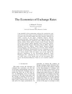
January 2011 revolution, where the exchange rate of Egyptian pound per Euro currency increased from 7.8 L.E. / € in 2011 to 8.7 L.E. / € in March 2013 (CBE monthly report April2013). The essence of the International Fisher Effect theory entails that the interest rates that are to be compared between different countries must have the same properties. Treasury bills (T- bills) being backed by the government, come closest to a risk free investment. Thus, T-bills across countries are considered perfect substitutes. It can be noted from Figureure (3) that the interest rate on Egyptian T-bills is always higher than that of US and German T-bills1. In the context of the IFE theory, real interest rates are supposed to be equalized across countries; accordingly, a high interest rate on Egyptian T-bills reflects expectation of a high inflation rate in Egypt. Thereby, the Egyptian pound is expected to be depreciating against both the US dollar and Euro currency. Accordingly, foreign investors are discouraged, since the interest rate differential is expected to be offset by the depreciation of the Egyptian pound. And this is what this paper is trying to examine. The impacts of the depreciation of the Egyptian pound on the economy vary between positive and adverse effects. The positive impact of depreciation is boosting exports. However, domestic firms that depend upon importing intermediate goods are disadvantaged. In addition, depreciation often creates expectations of future depreciation that weaken the domestic and foreign investors' confidence in the economy, triggering capital outflow (Abdel Haliem and El Ramly 2008). Another policy implication, if the IFE holds for Egypt, is the indication of free mobility of capital across borders, which have widespread benefits. Capital inflows in the form of FDI often bring improved technology, which raises productivity and growth. Besides, FPI flows increase market discipline and lead to a more efficient allocation of resources (Levine 1997). On the other hand, if the IFE doesn’t hold for Egypt, then the interest rate differential is not a predictive estimate for exchange rate. Also, this would imply that Egypt does not have free capital mobility. Accordingly, this paper aims at examining whether nominal interest rate differential is a good forecast for the changes in future spot exchange rate, in order to find out whether the IFE theory holds for the Egyptian economy. The paper is organized as follows. The second section reviews the theoretical literature of IFE theory. The third section highlights some of the empirical studies tackling the IFE theory. The fourth section presents the model and the data employed in investigating the relevance of IFE for Egypt, besides, explaining the methodology adopted. The fifth section displays the empirical results and interpretations. Finally, the sixth section concludes and provides some policy recommendations. 2. Theoretical Literature This section is divided into two parts. The first part reviews the theoretical foundation of the IFE theory. The second part discusses two opposing approaches for the relationship between nominal interest rate differential and nominal exchange rate changes that have conflicting implications. 2.1 Theoretical foundation of the IFE theory The theories of the Fisher Effect and Purchasing power parity (PPP) are the building blocks of the evolution of the IFE theory. Irving Fisher’s seminal article “The Theory of Interest” in 1930 is the corner stone of the Fisher hypothesis, which asserts that there is a positive correlation between a country’s nominal interest rates and its expected inflation; implying that the real interest rate is constant and independent of monetary measures. An extended version of this hypothesis is the Generalized Fisher effect (GFE) that takes into account the countries’ 1 Germany has been taken as a representative for the European Union because the European Central Bank reported in 2005 that Germany has the largest share of the European Union (EU) government debt securities issuance.

3

interactions. According to the GFE, the nominal interest rate differential between two countries is equal to their anticipated inflation differential. The country, which has the higher inflation rate, should bear higher interest rates relative to the lower interest rate country. Thus, in the absence of government intervention, capital flows towards the higher expected return country until expected real returns are equalized. Hence, capital mobility and capital market integration are important conditions for the GFE (Jeffy and Mandelker 1975). A crucial building block for the IFE theory is the PPP, which holds when exchange rate adjusts to offset the inflation rate differential between two countries. Hence, an increase in the price level of a country will cause depreciation of its exchange rate relative to other country, thereby keeping the relative price of identical goods the same across both countries (Madura 2009). However, the PPP might not hold in some countries due to that exchange rate movements might be affected by factors other than inflation differential; such as income level differential, expected changes in future exchange rate, terms of trade, balance of current and capital accounts, fiscal and monetary policies, and central banks interventions (Rosenberg, 2003). In addition, the PPP might not hold in case of absence of substitutes for traded goods. The IFE theory is the international counterpart of the Fisher Effect. It can be seen as a combination of the GFE and the PPP. The IFE uses interest rate differential rather than inflation rate differential to explain why exchange rate changes over time. The IFE2 theory asserts that foreign currencies with relatively high interest rates will depreciate because the high nominal interest rates reflect expected inflation (Madura 2009). It can be represented in the following equation: 1

(1)

In equation (1), the denotes the percentage change in the value of the foreign currency denominating the foreign security, while the and denote the home interest rate on home country securities and the foreign interest rate on foreign country securities respectively. IFE theory entails that when ih is greater than if, ef will be positive in which the home currency will depreciate with respect to the foreign currency due to high inflationary expectations in the home country. This depreciation will reduce the return on home securities, thereby, making returns on home securities no higher than foreign securities. The opposite should happen when ih is lower than if. Thus, the IFE theory implies a positive relationship between changes in the exchange rate and nominal interest rate differential. Accordingly, the essence of the IFE is that the spot exchange rate should change to adjust for differences in nominal interest rates between two countries. The adjustment can take place through two ways: either through flow of capital across international money markets or through trade and flow of goods across goods market (Sundqvist 2002). Thus, having free capital mobility is a must for the IFE to hold. However, since the IFE theory is based on the PPP theory, then IFE theory might not hold for the same reasons that prevent the PPP from prevailing. 2.1 The relationship between nominal interest rate differential and nominal exchange rate changes International finance theories encompass two opposing approaches to the relationship between nominal interest rate differential and nominal exchange rate changes. One approach, introduced 2

The International Fisher Effect Theory is also referred to as the Uncovered Interest rate parity. If the no-arbitrage condition is satisfied without the use of a forward contract to hedge against exposure to exchange rate risk, then interest rate parity is said to be uncovered. Investors are indifferent to the available interest rates in two countries because the exchange rate between those countries is expected to adjust such that the dollar return on dollar deposits is equal to the dollar return on foreign deposits.

4

by Frenkel (1976), assumed that prices are perfectly flexible, in which changes in the nominal interest rate reflect changes in the expected inflation rate. When the domestic interest rate rises relative to the foreign interest rate, demand for the domestic currency falls which causes it to depreciate instantly. Thus, there is a positive relationship between the changes in exchange rate and the nominal interest differential which conforms to the IFE theory. Dornbusch introduced (1976) and opposing approach that traced the adjustment of the exchange rate to interest rate differential over time. He assumed that goods prices are sticky and they adjust more slowly over time than financial asset prices. For instance, a rise in domestic money supply will result in a decline in domestic interest rate, and consequently, capital will outflow leading to depreciation in the domestic currency and overshooting its long run equilibrium level. However, over time the currency depreciation will reduce the relative price of domestic goods, stimulating the aggregate demand and inflationary pressures. Moreover, the excess money supply will also result in inflationary pressures. Hence, this will be reflected in an increase in the interest rate and appreciation of the exchange rate undoing the initial overshooting. Thus, there is a negative relationship between the changes in exchange rate and the nominal interest differential. This implies that Dornbusch (1976) is against the IFE theory. However, Frankel (1979) argued that nominal interest rate reflects both real interest rate and inflation. Thus, he developed the real interest rate differential model representing the relationship between changes in exchange rate and real interest rate differential. Frankel’s (1979) model incorporated the inflationary expectations element of the flexible price model with the sticky price element of the Dornbusch (1976) model and concluded that the exchange rate is negatively related to the real interest differential, but positively related to the expected long-run inflation differential. Several empirical studies followed Frankel (1979) and assessed the relationship between exchange rate changes and real interest rate differential (Meese and Rogoff 1988; Hoffmann and MacDonald, 2009). However, the focus of this paper is to study the relationship between nominal exchange rate changes and nominal interest rate differential under the umbrella of the IFE. 3. Empirical Literature The empirical literature highlights some empirical studies that examined the relevance of the IFE in the real world. The studies involve different countries, developed and developing ones and at different time spans. Sundqvist (2002) examined the IFE theory for the USA vs. five industrialized countries: Sweden, Japan, UK, Canada, and Germany. Interest rate differential was regressed against exchange rate changes for each case individually for the period 1993-2003. The empirical investigation revealed that the IFE theory holds for USA vs. Japan only. The author concluded there was an absence of a stable predictable relationship between exchange rate changes and interest rate differential. Ersan (2008) examined the IFE theory within a co-integration framework for Turkey with respect to the G-5 countries, namely USA, UK, Japan, France and Germany over the period 1985 -2007. The empirical estimation revealed that there is a long run relationship between nominal interest rate differentials and exchange rate changes. The IFE theory proved to hold for Turkey when it was included as home country against the other countries. However, the IFE didn’t hold for other country pairs, except for France & Germany. The author attributed this to the fact that perfect capital mobility might not been prevailing between the country pairs investigated. In addition to political risk, currency risk and transaction costs that affect investors’ decisions.

5

Shalishali (2012) investigated the IFE theory among eight industrialized countries, namely Indonesia, the Philippines, China, Japan, South Korea, Singapore Malaysia, and India over the period (1990-2009). Time series regression has been adopted. The empirical results were mixed between support and opposition to the IFE theory in which the theory held for some countries when used as home country and failed when they were used as foreign countries. The author attributed the results to other factors affecting the exchange rate rather than interest and inflation rates differentials, for instance, expected future exchange rate. Al-Nashar (2013) tested for the uncovered interest rate parity for Egypt through examining the stationarity of the exchange rate-adjusted interest rate differential between Egyptian and US three-month Treasury bill rates. Monthly data was employed for the period January 2000December 2011, as well as, for shorter period that had a surge in capital inflows from July 2004–June 2008. The Augmented Dickey Fuller (ADF) test for stationarity revealed nonstationarity of the exchange rate-adjusted interest rate differential for both periods concluding failure of uncovered interest rate parity to hold. The author attributed the results to the low degree of Egypt’s financial integration with international financial markets. In addition, investors are neither rational in their expectations about future spot exchange rate nor risk neutral; implying premium between domestic and foreign interest rates. Also, the variance decomposition of the interest rate spread between Egypt and USA, showed that, expected inflation differential was the largest contributor to the variation in the interest rate spread as affirmed by the Fisher theory. From the preceding empirical literature review, there isn’t a definite judgment for the validity of the IFE theory in predicting exchange rate fluctuations. The studies vary between supporting and opposing the IFE theory. As different countries, different time spans and different types of data have resulted in contradictory outcomes for the nominal exchange rate changes – nominal interest rate differential relationship. In addition, the level of financial development and capital market integration of countries affect the empirical results. Thus, the relevance of the IFE depends upon the individual case of each country and its macro-economic conditions. 4. Data and Methodology In light of the theoretical and empirical literature previously discussed in sections two and three; this section empirically assesses the validity of the IFE theory for the Egyptian case, with respect to USA and the European Union (EU). This section is divided into three parts. The first and second parts present the model and the data employed. The third part discusses the methodology adopted in the empirical analysis. 4.1 The Model Madura (1995) illustrated the derivation of the IFE model. The formula of effective return on a foreign money market investment is: 1

1

1

(2)

Where is the interest rate in the foreign country and is the rate of change in the value of foreign currency denominating the security. According to the IFE, , should equal , which is the effective return on a domestic money market investment (interest rate in the home country). Thus, substituting by for in Eq. (2) and solving for will result in the following equation:

(3)

Madura (1995) developed a statistical test of the IFE by applying regression analysis. The rate of change of spot exchange rate change over time is modeled as a function of the nominal interest rate differential as follows: 6

(4) is the interest rate differential.

where

is the constant indicating the rate of change in

the spot exchange rate when the interest rate differential is zero. is the regression coefficient indicating the rate at which the spot exchange rate will change in response to a change in interest rate differential. is the error term. According to the IFE theory, = 0 and = 1. Thus these are the hypotheses that will be tested in order to determine whether interest rate differentials are unbiased predictors of changes in exchange rates. 4.2 The Data 4.2.1 Dependent variable: rate of change in spot exchange rate (EX) Quarterly data for the rate of change in Egyptian pound per US dollar spot exchange rate and the rate of change in Egyptian pound per Euro spot exchange rate. The source of data is the CBE. The USA and the EU were chosen as the foreign countries because they are Egypt’s main trade partners. 4.2.2. Independent variable: nominal interest rate differential (INTDIFF) The T-bill rate will be used as a proxy for the nominal interest rate. Quarterly data for six months maturity for Egyptian T- bills, US T-bills and German T-bills will be employed. The source of the data is Bloomberg database. 4.2.3 Sample period The time span of the research will start from year 2003 up to year 2012. In January 2003, Egypt has stepped towards liberalizing the economy and the foreign exchange market, as a result of the CBE’s announcement to float the Egyptian pound. 4.3 The Methodology 4.3.1 Unit Root Test An econometric analysis usually starts with univariate analysis for the variables included in the model before empirical estimation. The ADF test will be employed to check for the stationarity of the variables under study. The ADF unit root test is undertaken through the following equation: ∆







1

∑

∆



(5)

Where Yt will be replaced by each of the model’s variables: rate of change in the spot exchange rate of Egyptian pound per US dollar.

/ /



rate of change in the spot exchange rate of Egyptian pound per Euro. ,

nominal interest rate differential between Egyptian and US six months

maturity T-bills. ,

nominal interest rate differential between Egyptian and German six months

maturity T-bills. refers to the trend and j refers to the no. of lags. The number of lags is chosen to minimize Akaike Information Criterion (AIC) and/or Schwartz Bayesian Criterion (SBC). The null hypothesis of ADF test is 0 1 indicating a non-stationary variable. The null hypothesis will be rejected indicating that the variable is stationary, if the estimated value of the ADF test statistic is less than Mackinnon critical values.

7

4.3.2 Autoregressive Distributed Lag (ARDL) bounds test approach to Co-integration and Error Correction Model (ECM) The research methodology will address both the long run and short run relationships between the nominal exchange rate changes and the nominal interest rate differential under the umbrella of the IFE theory. The approach that will be undertaken is the Autoregressive Distributed Lag (ARDL) bounds test approach to co-integration and error correction model (ECM) initiated by Pesaran et al. (2001). Co-integration refers to the long run equilibrium relationship between variables. Two non-stationary variables can be co-integrated if a linear combination of those variables is stationary (Engle and Granger 1987). Co-integration between variables implies the existence of an adjustment process referred to as “Error Correction” that prevents the errors in long run relationship from becoming larger and drifting apart from the equilibrium. The speed of adjustment toward equilibrium is determined by the ECM. Thus, ECM incorporates both short run dynamics and long run relationship between the variables. The advantage of Pesaran’s (2001) ARDL approach to co-integration over the conventional Engle and Granger (1987) and Johansen (1988) approaches to co-integration is that it overcomes the problem associated with the uncertainty of whether the series involved in the model are purely I(0), purely I(1), or mutually co-integrated. Pindyck and Rubinfeld (1998) asserted that despite the fact that the ADF test is widely used as a unit root test, the power of the test is limited. Moreover, the ARDL approach passes up the need to specify endogenous and exogenous variables, which is not the case for the conventional approach (Pesaran & Smith 1998). The ARDL approach also allows the variables to have different number of lags, which is not allowed in the conventional approach that sets the same number of lags for all the variables3. The ARDL model means that the dependant variable is expressed as a function of its own lagged values and the current and lagged values of the explanatory variable. The ARDL model of order p and n, ARDL (p, n), is defined as follows: ∑

(6)

∑

By rearranging the X’s obtained with, ∆, first difference operator, the following equation is obtained: ∑



1

∑



∑

(7)

∆

The use of this specification has been suggested for co-integration analysis by Pesaran and Shin (1998). Also, another transformation for the sake of co-integration testing is subtracting and making use of the fact that ∆ , which give the following equation: ∑

∑

∆



where and

are the long run parameters.

∆

(8)

∅∆

Thus, Pesaran’s (2001) augmented ARDL bounds testing approach to test for co-integration between rate of change of spot exchange rate (EX) and interest rate differential (INTDIFF) is given by the following equation: ∆





∑

∆

∑

∆ (9)

3

The case of this research is having two variables under study, so if co-integration exists then there will be one co-integrating vector. However, in case of having more than two variables, the conventional Johansen approach to co-integration estimates the long-run relationships within a context of a system of equations, while the ARDL method employs only one single reduced form equation.

8

Where is the intercept and εt is the white noise error term. and are the long run parameters, while p and n are the number of lags selected by minimizing AIC and/or SBC. The joint significant F-test or Wald statistic of the lagged level variables is employed for investigating the existence of the long run relationship among the variables. The null hypothesis of having no co-integration, H0: = = 0 is tested against the alternative hypothesis, H1: ≠ 0 and/or ≠ 0. The critical values for the F-statistic used are those tabulated by Pesaran et al. (2001) for different numbers of regressors. There are two sets of critical values, one upper bound and another lower one. The former refers to I (1) series and the latter to I (0) series. If the computed F-statistic exceeds the upper bound of the critical values, then the null hypothesis of no co-integration is rejected. If it is less than the lower bound value, then the null cannot be rejected. If it falls between the two levels of the bands, then cointegration test becomes inconclusive. Also, Narayan (2004) introduced a reformulation for the critical values for the bounds F-statistic initiated by Peseran (2001), in order to fit small data sets, between 30 and 80 observations. If a long-run relationship is established between the variables, then short run dynamics derived from an error correction model (ECM) can be estimated from the following equation: ∆



∑

∆

∑

∆





(10)

Where is constant, is error term, and are coefficients of the short run dynamics, while measures the speed of adjustment to long run equilibrium. is the lagged error correction term derived from the following long run equation: (11) 4.3.3 Granger Causality test In addition, the Granger causality test will be conducted to examine the direction of the relationship between EX and INTDIFF. The intuition of this test is to investigate if INTDIFF granger causes EX, then the past values of INTDIFF can be used to predict changes in EX. On the other hand, if EX granger cause INTDIFF, then the past values of EX can be used to predict changes in INTDIFF. If a long run relationship between EX and INTDIFF is found in eq. (9) according to the previously explained ARDL bounds test, then the ECM estimated in eq. (10) can be used to test for the causality running from INTDIFF to EX, by testing the following null hypotheses (Granger 1988; Mehrara 2007): 

Short-run Granger causality: (Ho: ⋯ 0) tests for the significance of the coefficients of the independent lagged variable –INTDIFF- in eq. (10), in order to assess Granger weak causality which is interpreted as short run causality, since the dependant variable will be responding only to short term shocks (Masih and Masih 1996).  Long-run Granger causality: (Ho: 0), in which, , is the coefficient of the error correction term in eq. (10), representing the speed of adjustment to long run equilibrium. If 0, then EX does not respond to a deviation from the long run equilibrium in the previous period.  Strong Granger causality: (Ho: ⋯ 0), to check whether the two sources of causation – short run and long run – are jointly significant, in order to test for Granger causality. However, if the long run relationship is not found, then Granger causality can be examined through a Vector Autoregressive (VAR) model by running eq. (10) after excluding the error correction term and testing for short run Granger causality only (Jenkins and Katircioglu 2010). On the other hand, testing for the causality running from EX to INTDIFF, implies running an equation similar to eq. (9) but using INTDIFF as the dependent variable and EX as the independent one, and testing for the long run relationship through the ARDL approach to co9

integration. If co-integration exists, then ECM can be estimated and used to test for the Granger causality running from EX to INTDIFF. However, if co-integration doesn’t exist, then testing for Granger causality can take place through a VAR model. 4.3.4 Impulse response function (IRF) and variance decomposition (VD) Though, the ECM estimated in eq. (10) incorporates the long run and short run relationships between EX and INTDIFF, there is still a need to study the dynamics of this relationship in the short run and its projections. Therefore, a VAR model will be estimated and interpreted through the impulse response function (IRF) and the variance decomposition (VD) both of which can effectively capture the short run dynamics. The IRF traces the response of an endogenous variable to a shock in that variable and in every other endogenous variable. As for the VD, it breaks down the variance of the forecast error for each variable into components that can be attributed to each of the endogenous variables. The VD can, therefore, indicate the relative importance of interest rate differential in determining changes in exchange rate. The preceding methodology will be adopted to examine the existence of the IFE once for the case of Egypt vs. USA and another time for the case of Egypt vs. Germany. 5. Estimation Results and Interpretation Prior to reporting the estimation results, ADF unit root results will be reported for the four variables under study to check for their stationarity and order of integration. Although the ARDL approach to co-integration doesn’t prerequisite a unit root test, however, it would work as evidence about whether or not the ARDL approach is the appropriate approach to be undertaken. In addition, a unit root test will be undertaken to ensure that the variables under study are either I (0) or I (1); because critical values of the F-test of the ARDL approach to cointegration is bounded between I(0) and I (1), so it won’t be relevant if a variable is integrated of order two, I (2). Consequently, this section is divided into six parts. The first part reports the unit root test results. The second part presents the estimation results of ARDL approach to cointegration and ECM. The third part provides the results of the Granger causality test. The fourth part displays the IRF and VD. The fifth part provides robustness test. Finally, the sixth part discusses the interpretation of the results for each case individually. 5.1 ADF unit root test ADF test has been employed to test for the stationarity of the variables under study. Table (1) shows that and and / / are stationary series, while , are first order homogenous, I (1). , 5.2 Autoregressive Distributed Lag (ARDL) approach to Co-integration and Error Correction Model The preceding ADF unit root test results supports the choice of the ARDL approach to cointegration due to the fact that the variables under study have different orders of integration. ARDL (1, 1) – one lag for each variable – is chosen as it minimizes AIC & SBC. Thus, the following ARDL model was estimated once for the case of Egypt vs. USA and another time for the case of Egypt vs. Germany: ∆

∆



∆



∆ (12)

An coefficient test is carried for and using Wald test. The F-statistic is significant for both cases as shown in Table (2) and accordingly has to be compared to the tabulated critical value bounds of F-statistic reported by Paseran (2001). Also, F-statistic will be compared to critical value bounds of Narayan (2004). For the case of Egypt vs. USA, the F-statistic exceeds the upper bound of the tabulated F- critical bound for both Paseran (2001) & Narayan (2004). Hence, the null hypothesis of no co-integration is rejected supporting the existence of a long 10

run relationship between and . Same applies for the case of Egypt ⁄ , and vs. Germany. Therefore there also exists a long run relationship between ⁄ . , Since co-integration exists, then the long run model can be estimated as follows:





(13)



Where the null hypothesis of IFE is

= 0 and

=1.

In the case of Egypt vs. USA, Table (3) shows that, , the long run coefficient of , is 0.37. This means that a one percent increase in the interest rate , differential between Egyptian and US T-bills will result in a 0.37 percent increase (depreciation) in the exchange rate L.E./$. The value is positive conforming to the IFE theory and significant at 10% level as pointed by the p-value. However, it is less than unity, far from the null hypothesis concluding partial significance of the IFE in the case of Egypt vs. the USA. Accordingly, if interest rates in Egypt are higher than that in the USA, then the Egyptian pound will depreciate, however, American investors might still gain profits from investing in Egyptian securities since the interest rate differential isn’t equally offset by the depreciation in Egyptian pound. While, in the case of Egypt vs. Germany, Table (3) shows that, , the long run coefficient of is negative and insignificant as indicated by the t-statistic and the P-value. , Therefore, real interest rates are not equalized between Egypt and Germany, consequently, there exists opportunities for abnormal gains in portfolio diversification between them in the long run. Accordingly, the IFE doesn’t apply in the case of Egypt vs. Germany. Since co-integration exists, then an error correction model can be estimated as follows: ∆ here

∆ ∆ ∆ is the residual of the long run model in Table (3) lagged once.



(14)

In the case of Egypt vs. USA, Table (4) reports the speed of adjustment to long run equilibrium between the interest rate differential and exchange rate changes. It is measured by, , the coefficient of error correction term (ECt-1) which, is highly significant as indicated by the tstatistic and the P-value. It implies that 72 percent of the deviation from the long run path between and in period t-1 will be compensated in period t. , / As for the case of Egypt vs. Germany, Table (4) shows that the speed of adjustment to long run equilibrium is negative and highly significant as pointed by the t-statistic and the P-value which strengthens the long run negative relationship between and . The , / absolute value of the speed of the adjustment is greater than one which implies overshooting the equilibrium level. Therefore, there exists opportunities for arbitrage profits in portfolio diversification between Egypt and Germany in the long run. 5.3 Granger causality test The direction of the relationship between EX and INTDIFF was estimated by the Granger causality test. Both directions were examined. 5.3.1 First hypothesis: INTDIFF granger does not cause EX A long run relationship was found between EX and INTDIFF when EX was taken as the dependant variable in the ARDL approach to co-integration for both cases: Egypt vs. USA and Egypt vs. Germany. Accordingly, the hypothesis: INTDIFF granger does not cause EX was examined by testing for the significance of the coefficients of the parameters of the ECM reported in Table (4). Three hypotheses were tested: long run causality, short run causality and strong causality as shown in Table (5). The results revealed the same findings for both cases. 11

The error correction term was significant indicating the presence of long run causality. However, the lagged INTDIFF was insignificant indicating the absence of short run causality. Yet, the joint significant F-statistic for both short run and long run parameters was significant implying strong causality running from INTDIFF to EX which is attributed to a long run causality rather than a short one. 5.3.2 Second hypothesis: EX granger does not cause INTDIFF A long run relationship wasn’t found between EX and INTDIFF when INTDIFF was taken as the dependant variable using the ARDL approach to co-integration for both cases: Egypt vs. the USA and Egypt vs. Germany. The results are reported in appendix A. Accordingly, the hypothesis: EX granger does not cause INTDIFF, was examined by a VAR model in which the null hypothesis was not rejected in both cases as reported in Table (6). Hence, the relationship between EX and INTDIFF is unidirectional running only from INTDIFF to EX. Thus, then the past values of INTDIFF can be used to predict changes in EX conforming to the IFE theory. 5.4 Impulse response function and variance decomposition Short run dynamics between and can be examined by estimating a VAR model and interpreting it through IRF & VD. IRFs are reported for 10 quarters in Figure. (4) for the case of Egypt vs. the USA & in Figure. (5) for the case of Egypt vs. Germany. For the case of Egypt vs. the USA, Figure.(4) shows that increases slightly in response to one / in the second quarter, and then the effect of the standard deviation shock in , shock dampens out and fades away by the fourth quarter. Thus, the negligible effect of the shock in on , implies the absence of a short run relationship. This , / IRF result supports the granger causality test result which entailed the absence of short run causality running from to . , / decreases in response As for the case of Egypt vs. Germany, Figure. (5) shows that / reaching a trough by the end of the third quarter, then increases to a shock in , gradually during the fourth quarter but dampens out and fades away by the seventh quarter. Therefore, the IFE doesn’t hold in the short run for the case of Egypt vs. Germany. This result matches the long run result that found a negative relationship between changes in the exchange rate and interest rate differential between Egypt and Germany. Regarding the VD, Table (7) reports the VD for 10 quarters forecast of EX / in which shocks, while 0.12 percent to 99.8 percent of the forecast variance is attributed to / shocks. On the other hand, 10 quarters forecast of VD of , indicates , / shocks, while 6.18 percent that 93.82 percent of the forecast variance is attributed to / . The VD results imply that INTDIFF has a negligible effect on EX in the to , short run for both cases; the Egyptian pound with respect to the US dollar and the Egyptian pound with respect to euro currency. Hence, the VD results support both the IRF results and Granger causality test results which revealed an absence of short run causality running from INTDIFF to EX in both case studies. 5.5 Robustness test In order to check the sensitivity of the results to the model specification, the relevance of the IFE was further tested using another Euro area member country, namely France. The results of the ARDL approach to co-integration are reported in appendix B. They indicated the irrelevance of the IFE in the case of Egypt vs. France. This conforms to the results of Egypt vs. Germany and emphasizes that the empirical results are robust with regard to the chosen Euro area member country.

12

5.6 Interpretation of the results This section interprets and analyses collectively the findings of the long run – co-integration and error correction– and the short run – VAR analysis– estimation results in an attempt to find out the reasons preventing the IFE to hold in Egypt. This section is divided into two parts in which each of the cases of Egypt vs. the USA and Egypt vs. Germany is analyzed individually. 5.6.1 Egypt vs. the USA The preceding long run and short run estimation results revealed that the IFE partially exists in the case of Egypt vs. the USA. Although, the results revealed a positive significant relationship between changes in the exchange rate and interest rate differential which conforms to the IFE theory. However it wasn’t a one to one relationship. Thus, there might be a tendency of American purchases of Egyptian debt securities, since the interest rate differential is not equally offset by the change in exchange rate. The failure to have the full IFE might be attributed to several reasons. One reason is that the IFE is based on the PPP theory, if the PPP doesn’t hold then the IFE is not likely to hold. Accordingly, the relevance of the PPP theory for the case of Egypt vs. the USA was investigated over the period 2003-2012. The results are reported in appendix C. The results imply that the PPP is not holding in the case of Egypt vs. the USA. The inflation rate is higher in Egypt than in the USA; however the controversy is that the USA imports necessary goods from Egypt thus hindering the PPP. The Egyptian exports to USA accounted for 35.4% of Egypt’s total exports in FY2002/2003. This percentage reached 12.7 % of total exports in FY2011/2012 (CBE annual reports). The USA is the main trade partner for Egypt after EU. Moreover, trade barriers might be hindering the PPP to hold. Although liberalization is taking place in Egypt, in which tariff rates were reduced from 14.6 percent to 5.5 percent as part of the economic reforms that Egypt embarked on beginning in 2004. However, non tariff barriers still exist affecting the flow of goods from USA to Egypt. Another possible reason for the irrelevance of the IFE in Egypt is the persistence of high inflation rates in Egypt that have raised the interest rates; on the other hand, the USA has had very low interest rates throughout the period of study. The FED lowered the federal fund rate to one percent during 2003-2004 in order to boost up the economy after the invasion in Iraq. As well, the financial crisis drove the FED to set federal fund rate to around zero percent since 2008. This low rate of return pushed the American people, seeking higher nominal rates of return, to look for higher yielding foreign assets (Kliesen 2010). Thinking in terms of nominal rather than real monetary values is referred to as money illusion. In this respect, Egypt was one of the countries that attracted investors seeking high nominal returns. From the CBE annual reports, it can be noticed that international reserves had a substantial increase from 14.3 billion $ in FY2003/2004 to 34.6 billion $ in FY 2007/2008. The expansion in the international reserves was attributed to the increase in oil prices, Suez Canal revenues and upsurge in FDI and FPI inflows. Also, the IFE might not be taking place due to the fact that the exchange rate of L.E. /$ is not allowed to float freely. The exchange rate only experienced 30% depreciation immediately after the announced floatation in 2003. And then throughout the period of surge in capital inflows (2005-2008), the exchange rate was expected to be vulnerable to high volatility. However, it was nearly stable with 9 percent appreciation due to the sterilized foreign exchange intervention by the CBE in order to avoid exchange rate appreciation. The IMF (2007) reported that sterilization measures accounted for one percent of GDP in 2007. Foreign flows were partially sterilized stimulating inflation rate and pushing interest rates upward and in turn raising interest rate differential (Selim 2012). 13

Selim (2012) was concerned with the effect of sterilization on the free willingness of exchange rate and estimated a de facto classification for Egypt’s exchange rate regime for the period of 1982-2008. The estimation revealed that the exchange rate can’t be classified as float after the FY 2003/2004. This is supported by the IMF (2007) de facto classification of Egypt’s exchange rate, in which the regime has been classified as a managed float with a pre-determined path for the exchange rate since 2003. More recently, the IMF Country Report 2010 stated that the Egypt exchange rate regime became “other managed arrangements”.4 Nevertheless, Ray (2012) argued that even in a regime of fixed exchange rate and perfect capital mobility, real interest rates will be equal across markets implying that the IFE would hold. However, in a regime of flexible exchange rates where the capital market is imperfect, real interest rates difference persists opposing the IFE. Hence, there is the question of Egypt having free capital mobility in which capital integration between Egypt and the US exists. Marashdeh (2005) examined the financial integration between MENA countries namely, Egypt, Turkey, Jordan and Morocco, and developed markets represented by the USA, UK and Germany. He found that MENA countries’ stock markets are co-integrated while no cointegration exists between MENA investigated countries markets and developed markets except for Egypt during 1994-2004. However, Segot and Lucey (2007) had opposing results. Furthermore, Al-Nashar (2013) used the capital account openness index (KAOPEN), initiated by Chinn and Ito (2006)5, to measure Egypt’s degree of de jure financial account openness. The author compared Egypt’s de jure financial openness with the flows of FPI; as she asserts that FPI is the most relevant proxy for the de facto financial openness. KAOPEN index recorded a steady score of 2.44 during the period from 2004 - 2008 – concurrently with banking and financial reforms that took place at that time – which is the highest score compared to industrial countries such as the USA, UK and European countries that had the same score of 2.44. Accordingly, Egypt witnessed a surge in capital inflows during 2005-2008. However, the index recorded a gradual decline for Egypt compared to industrial countries during the period of 2009-2011, reaching 1.65 in 2011 due to Egypt’s measures to hedge the risk associated with the global financial crisis and the adverse economic repercussions of the January 2011 revolution, where this period witnessed a capital outflow. Hence, despite of the de jure financial openness in Egypt, FPI net inflows witnessed high volatility since the early 2000s up till today; implying that the de facto financial openness was limited. Al-Nashar (2013) further investigated the de facto capital and financial openness in Egypt empirically by making use of the impossible trinity framework. This trinity asserts that if there is a fixed exchange rate and free capital mobility then it is impossible to have an autonomous monetary policy in which central banks can’t influence interest rates. Regarding Egypt, the exchange rate is nearly stabilized as previously explained by Selim (2012) and IMF reports, besides, the KAOPEN index shows a de jure financial openness. Hence, Al-Nashar (2013) assessed the monetary autonomy for Egypt and found that the growth rate in the monetary aggregate (M2) –proxy for money supply– Granger causes movements in the exchange rateadjusted interest rate differential for the periods (2000-2011) and (2004-2008), implying that CBE is preserving its monetary autonomy. Accordingly, Egypt’s monetary autonomy can’t be preserved unless financial integration/capital mobility is imperfect implying limited de facto financial openness.

4

“other managed arrangement” this category captures countries in which the de facto and the de jure arrangement differ, which manage their exchange rates but are not floating, and which exhibit frequent or irregular changes in policies. 5 KAOPEN is based on the binary dummy variables that codify the tabulation of restrictions on cross boarder financial transactions reported in the IMF's Annual Report on Exchange Arrangements and Exchange Restrictions (AREAER), for more details see, Chinn and Ito (2006).

14

In this context, IMF Country Report of 2010 affirmed that the fact that the financial system in Egypt is less integrated with the global economy compared to the real sector was the reason behind Egypt’s quick recovery from the global financial crisis compared to other countries at the same income level. This is in addition to the CBE’s Phase I reforms (2004 - 2008) – banks’ restructuring, consolidation, and cleanup of non-performing loans – which reduced financial vulnerabilities. However, Kosea et al. (2011) attributed a country’s limited de facto financial openness and integration to the fact that there is a threshold of financial depth and institutional quality that an economy has to attain, in order to witness financial integration. In this respect, Reda (2012) found that Egypt’s banks’ consolidation had a positive effect on managerial efficiency, capitalization and risk management practices, yet financial depth and banks’ intermediation, as reflected by loans to deposits ratio, and banks profitability have weakened. Moreover, Nasr (2009) affirmed that Egypt’s institutional infrastructure is still not well acquainted with the targeted financial integration. For instance, there are no specialized courts for financial institutions, and no specialized judges with adequate knowledge of financial market risks. That is why Egypt had a moderate rank in the financial development index6 published by World Economic Forum in its first financial development report in 2008. Egypt ranked 37 with a score of 3.3, while the US was the top ranked with a score of 5.8. Emerging economies were having higher ranks than Egypt. Countries with emerging economies increased their ranking in the financial development report in 2010 while Egypt remained at the same rank. Also, European countries such as Germany were highly ranked compared to Egypt. Furthermore, the justification that might be behind the delayed financial integration and in turn insignificance of the IFE is that the route towards financial integration requires sequential prerequisites as indicated by Jedidi and Mensi (2010) based on their empirical investigation of MENA countries. Their findings emphasized that trade openness must be implemented five years before capital account liberalization and a year after achieving macroeconomic stability. Also, a satisfactory level of economic development, and an inflation control of five years preceding liberalizing capital account, must accompany banking system development. In addition, stock market development, as reflected in the performance and the size of its capitalization, must be accompanied by an inflation control process four years in advance. It can be inferred from Jedidi and Mensi (2010) that throughout the period of 2003-2012, Egypt had trade openness. However, Egypt didn’t experience full 5 years of controlled inflation and satisfactory economic development in terms of GDP, even before 2003. Therefore, Egypt hasn’t fulfilled the prerequisites of financial openness, which hinders the IFE to hold. It is worthy to note that Egypt has plunged into a political and economical transition subsequent to January 2011 revolution. The banking and financial sectors were affected due to the successive downgrading to Egypt’s sovereign credit rating by three credit rating agencies7 dating from the revolution till today. The downgrading affected the soundness of the financial sector in Egypt leading to capital outflows and decreasing the investors’ confidence in the Egyptian economy, all of which negatively affected the financial development in Egypt. Also, psychological barriers might hinder the IFE. Besides, legal restrictions and transaction costs act as barriers (Solnik 2000). Further, the currency risk and tax on yields influences the flow of capital. 6 Financial development index has a score range (0-7). It ranks 52 of the world’s leading financial systems. The World Economic Forum defines financial development as “the factors, policies, and institutions that lead to effective financial intermediation and markets, and deep and broad access to capital and financial service”. 7 The three credit rating agencies that downgraded Egypt’s sovereign credit rating sixteen times since January 2011 revolution are as follows: Standard & Poor downgraded Egypt’s sovereign credit rating from BB+ to CCC+, Moody’s downgraded from Ba1 to Caa1and Fitch downgraded from BB+ to B.

15

5.6.2 Egypt vs. Germany Long run and short run estimation results revealed that IFE doesn’t hold for the case of Egypt vs. Germany. This implies that exchange rate of the Egyptian pound per Euro doesn’t offset the interest rate differential between Egypt and Germany. In this respect, German investors are attracted to the high interest rates of Egyptian securities resulting in appreciation in the exchange rate of L.E./ €. As explained previously, the failure to have the IFE might be attributed to several reasons including the irrelevance of the PPP. To the extent of the authors’ knowledge, the empirical literature hasn’t examined the PPP theory between the Euro currency and the Egyptian pound. Thus, this paper tested for long run PPP between the Egyptian pound and the Euro over the period of 2003-2012. The results are reported in appendix C. The results implied the failure of the PPP to hold between the Egyptian pound and the Euro currency. The PPP might be invalid because the EU is the main trade partner with Egypt. Although the inflation rate is higher in Egypt than in the EU, Egypt’s exports to the EU account for more than 30 percent of Egypt’s total exports throughout the studied period. Egypt is ranked the fifth exporter to the EU in the region in 2011. Moreover, the trade between Egypt and the EU was further intensified and supported by the EU-Egypt Association Agreement that came into force in 20048. Afterwards, a joint EU-Egypt Action Plan was established in 2007 which set an agenda for intensified relations between the two sides in the context of the European Neighborhood Policy (ENP). Accordingly, Egypt acquired about an €558 million financial assistance package for the period 2007-2010 to facilitate economic and social reforms. This flow of financial assistance to Egypt might have triggered the appreciation of the exchange rate of L.E. / €. Furthermore, in of 2003-2012, the European Central Bank (ECB) succeeded in keeping inflation around 2 percent in accordance to ECB’s objective of price stability. This stable inflation led the ECB to keep the key interest rates low through most of the studied period. The low interest rates might have pushed the European investors seeking high nominal interest rates to approach foreign high yielding asset even if they were riskier than domestic ones. Besides, there are other factors that could have hindered the IFE to hold, that were explained in detail in the case of Egypt vs. the USA. These factors include Egypt’s limited financial integration with international financial markets. In addition, money illusion, currency risk and political risk, as well as, the adverse impacts of the January 2011 revolution on the financial sector in Egypt. 6. Conclusion This paper aimed at examining the IFE theory, which implies that foreign currencies with relatively high interest rates will depreciate because the high nominal interest rates reflect expected inflation. Two case studies – Egypt vs. the USA and Egypt vs. Germany – were investigated during the period (2003-2012). The empirical findings revealed partial significance of the IFE in the case of Egyptian pound vs. the US dollar, while no sign of the IFE was detected in the case of Egyptian pound vs. Euro currency. The insignificance of the IFE in both cases has been attributed to the insignificance of the PPP in which exchange rate didn’t offset the inflation differential and thereby didn’t offset the interest rate differential. Consequently, it would be difficult to utilize the interest rate differential to forecast future changes in the exchange rate. In addition, the irrelevance of IFE implied that Egypt is having limited financial integration with international financial markets. In addition, money illusion, currency risk and political risk as well as the adverse economic 8

This agreement established a free trade area between Egypt and EU and abolished gradually the custom tariffs on industrial and agricultural products. Besides, this agreement facilitated movement of capital between the two partners. However, the non tariff barriers might be affecting the flow of goods from EU to Egypt.

16

repercussions of the January 2011 revolution on the banking and financial sectors in Egypt can all attribute to the failure of IFE to hold. Policy recommendations can be deduced from the preceding findings to the policy makers in Egypt. Policy makers need to have a look at eliminating the non-tariff barriers in order to allow free movement of goods and thereby permit the PPP to hold which is the building block for the IFE to hold. Furthermore, interventions in the foreign exchange market would have to be ceased because these interventions overvalue the Egyptian pound and hold back the ability of the exchange rate to adjust to inflation differential and interest rate differential; hindering the PPP and the IFE to hold. Despite of Egypt’s steps towards trade openness and banking reforms in two phases in 2004 and then in 2009, yet more effort is needed to enhance the financial depth in the Egyptian economy. Macroeconomic instability is still noticed, in which policy makers need to work on curbing down the inflation rate, stabilizing the output around its potential, and providing a friendly investment environment in order to encourage sustained foreign investment and economic growth. This is in addition to retaining the regional and global confidence in the Egyptian banking sector and financial system after the successive downgrading of the sovereign credit rating in the wake of the economic chaos subsequent to January 2011 revolution. Nevertheless, there are wide benefits from taking steps towards financial integration in terms of development in the domestic financial system, as well as, free capital mobility that stimulates capital and technological accumulation and consequently enhances economic growth. Supporting institutions and conditions need to be in place to mitigate the risk associated with fluctuations in capital flows. Hence, policy makers in Egypt are recommended to allow gradual and cautious financial openness until financial markets become well established, developed, and capable to hedge risk efficiently.

17

References Abdel-Haleim, S.M., EL-Ramly, H. 2008. “The Effect of Devaluation on Output in the Egyptian Economy: A Vector Autoregression Analysis.” International Research Journal of Finance and Economics 14. Al-Nashar, S.B. 2013. “On Egypt’s de facto Integration in the International Financial Market.” Egyptian Center for Economic Studies (ECES) working paper No. 174. Bahmani-Oskooee, M., Tankui, A. 2008. “The black market exchange rate vs. the official rate in testing PPP: Which rate fosters the adjustment process?” Economic Letters 99:40-43. Central Bank of Egypt (CBE). Annual Reports. Various issues. Central Bank of Egypt, Monthly Report, April 2013. Chinn, M.D., Ito, H. 2006. “What Matters for Financial Development? Capital Controls, Institutions, and Interaction.” Journal of Development Economics 81:163-192. Drine, I., Rault, C. 2008. “Purchasing Power Parity for Developing and Developed Countries. What can we Learn from Non-Stationary Panel Data Models?” Journal of Economic Surveys, 22 (4):752-773. Dornbusch, R. 1976. “Expectations and Exchange Rate Dynamics.” Journal of Political Economy :1161-1176. Ersan, E. 2008. “International Fisher Effect: A Reexamination within the co-integration and DSUR frameworks.” Master of Business Administration thesis submitted to the Graduate school of Social Sciences of Middle East Technical University. Financial Development Report 2008, World Economic Forum. Financial Development Report 2010, World Economic Forum. Fisher, I. 1930. The Theory of Interest. MacMillan, New York. Frankel, J. 1979. “On the mark: a Theory of floating exchange rates based on real interest differentials.” American Economic Review 69: 610–622. Frenkel, J. 1976. “A Monetary Approach to the Exchange Rate: Doctrinal Aspects and Empirical Evidence.” Scandinavian Journal of Economics 78: 200-224. Granger, C.W.J. 1988. “Some Recent Developments in the Concept of Causality.” Journal of Econometrics 39:199-211. Hoffmann, M., MacDonald, R. 2009. “ Real exchange rates and real interest rate differentials: A present value interpretation.” European Economic Review 53: 952–970. IMF (International Monetary Fund). 2007. Country Report No. 07/380, December. IMF (International Monetary Fund). 2010. Country Report No. 10/94, April. Jedidi, F.K. and Mensi, S. 2010. “Pre-requisites for Capital Account Openness: Empirical Validations of an Optimal Sequencing Model for the MENA Region Countries.” International Research Journal of Finance and Economics 54. Jeffrey, F.J, Mandelker, G 1975. “The "Fisher Effect" for Risky Assets: An Empirical Investigation.” The Journal of Finance 31 (2). Jenkins, H.P., Katircioglu, S.T. 2010. “The bounds test approach for co-integration and causality between financial development, international trade and economic growth: the case of Cyprus.” Applied Economics 42:1699–1707.

18

Johansen, S. 1998. “Statistical analysis of co-integration vectors.” Journal of Economic Dynamics and Control 12:231_254. Kleisen, K.L. 2010. The Regional Economist: 6-7. Kosea, M.A., Prasad, E.S., Taylor, A.D. 2011. “Thresholds in the process of international financial integration.” Journal of International Money and Finance 30:147–179. Levine, R. 1997. “Financial Development and Economic Growth: Views and Agenda.” Journal of Economic Literature XXXV:688-726. Madura, J. 1995. International Financial Management. . St. Paul: West Publishing Company. Madura, J, 2009. International Financial Management. South-Western College Publishing. Marashdeh, H. 2005. “Stock Market Integration in the MENA Region: An Application of the ARDL Bounds Testing Approach.” University of Wollongong Economics Working Paper Series, WP 05-27. Masih, A.M.M., Masih, R. 1996. “Energy consumption, real income and temporal causality: results from a multi-country study based on co-integration and error-correction modeling techniques.” Energy Economics 18:165–183. Meese, R., Rogoff, K. 1988. “Was it real? The exchange rate-interest differential relation over the modern floating rate period.” Journal of Finance 14:3–24. Mehrara, M. 2007. “Energy consumption and economic growth: The case of oil exporting countries.” Energy Policy 35:2939–2945. Narayan, P.K. 2004. “Reformulating critical values for the bounds F-statistics approach to cointegration: an application to the tourism demand model for Fiji.” Department of Economics Discussion Papers No. 02/04, 2004, Monash University, Melbourne, Australia. Nasr, S. 2009. “Are Banks in Egypt Catalysts for Economic Development?” Paper presented in Oxford Business & Economics Conference (OBEC) June 24-26, 2009, Oxford University, UK. Pesaran, H. M., Smith, R. 1998. “Structural analysis of co-integration VARSs.” Journal of Economic Surveys 12:471-505. Pesaran, H. M. et al. 2001. “Bounds testing approaches to the analysis of level relationships.” Journal of Applied Econometrics 16:289- 326. Pindyck, R.S., Rubinfed, D.L. 1998. Econometric Models and Economic Forecasts, Boston, MA: Irwin-McGraw Hill. Ray, S. 2012. “Testing the Validity of Uncovered Interest Rate Parity in India.” Advances in Applied Economics and Finance 1(4). Reda, M. 2012. “Measuring Banking Efficiency post consolidation: The Case of Egypt.” Egyptian Center for Economic Studies (ECES), working paper no. 173. Rosenberg, M. 2003.Exchange Rate Determination: Models and Strategies for Exchange Rate Forecasting. McGraw-Hill Library of Investment and Finance. Sabri, N.R., Peeters, M., Abulaben D.K. 2012. “The impact of exchange rate volatility on trade integration among North and South Mediterranean countries.” Munich Personal RePEc Archive MPRA Paper No. 38080. Segot, T. L., Lucey, B.M. 2007. “Capital Market Integration in the Middle East and North Africa.” Emerging Markets Finance and Trade 43(3):34-57.

19

Selim, H. 2012. “Has Egypt’s Monetary Policy changed after the float?” Middle East Development Journal,4(1). Solnik, B. 2000. International investment. NewYork: Addison Wesley Longman, Inc.

20

Figure 1: Annual Exchange Rate of Egyptian Pound per US Dollar

Source: Calculations by the authors

Figure 2: Annual Exchange Rate of Egyptian Pound per Euro Currency 8.4 8.0 7.6 7.2 6.8 6.4 2002 2003 2004 2005 2006 2007 2008 2009 2010 2011 2012 Source: Calculations by the authors

21

Figure 3: Interest Rate on 6 Month Maturity Egyptian T-Bills, US T-Bills and German T-Bills Interest rate on 6 months maturity T-bills

16 12 8 Egyptian T-bills German T-bills US T-bills

4 0 -4 2003 2004 2005 2006 2007 2008 2009 2010 2011 2012

Source: Done by the authors based on data from Bloomberg database.

Figure 4: Egypt vs. the USA Impulse Response Function Response to Cholesky One S.D. Innovations Response of EX(Eg/US) to EX(Eg/US)

Response of EX(Eg/US) to INTDIFF(Eg,US)

.020

.020

.016

.016

.012

.012

.008

.008

.004

.004

.000

.000

-.004

-.004 1

2

3

4

5

6

7

8

9

10

1

2

3

4

5

6

7

8

9

10

Figure 5: Egypt vs. Germany Impulse Response Function Response to Cholesky One S.D. Innovations Response of EX(Eg/EU) to EX(Eg/EU)

Response of EX(Eg/EU) to INTDIFF(Eg,Gr)

.06

.06

.05

.05

.04

.04

.03

.03

.02

.02

.01

.01

.00

.00

-.01

-.01

-.02

-.02 1

2

3

4

5

6

7

8

9

10

1

2

3

4

5

6

7

8

9

10

22

Table 1: ADF Unit Root Test Results Level Variable

EX

ADF test Statistic

INTDIFF EX

-14.2701 at trend * -0.382707

/

/

,

INTDIFF

,

First Difference ADF test Statistic Mackinnon(1996) critical values at 5% significance level -11.56549 -1.949856

Mackinnon(1996) critical values at 5% significance level -3.52976 -1.949609

-4.718334

-1.949856

-7.05089

-1.94961

-5.121004 (4)**

-1.951

-2.82605 at trend*

-3.52976

-5.07363

-1.94986

Notes: * Trend is significant for EX

/

at level and INTDIFF

at level. **The number between brackets ( ) refers

,

to the number of lags.

Table 2: F-Statistic of Co-Integration Relationship Egypt vs. USA F-Test Statistic

P-value

13.12331

0.0001

Egypt vs. Germany F-Test Statistic

P-value

14.12881

0.0000

Pesaran (2001) tabulated critical value bounds for Fstatistic at 5% significance level at restricted intercept and no trend

Narayan (2004) tabulated critical value bounds for Fstatistic at 5% significance level at restricted intercept and no Trend at n**=38

k*

I(0)

I(1)

K

I(0)

I(1)

1

3.62

4.16

1

5.807

6.490

Notes: *k refers to the no. of regressors which in this case is equal to one. **n refers to the number of observations

Table 3: Long Run Output EX

⁄

Egypt vs. USA 0.022365 0.369016 INTDIFF

Std. Error 0.018188 0.19452 t-statistic -1.229706 1.89706 Prob. 0.2264 0.0654 R-squared 0.086513 Adjusted R-squared 0.062474 F-statistic 3.598838 Prob. (F-statistic) 0.065439 S.E. of regression 0.044988 Durbin Watson Stat 0.757008

,

EX

⁄

Egypt vs. Germany 0.029403 0.165361INTDIFF

,

Std. Error 0.03087 0.335882 t-statistic 0.952458 -0.492319 Prob. 0.3469 0.6253 R-squared 0.006338 Adjusted R-squared -0.019811 F-statistic 0.242378 Prob. (F-statistic) 0.625326 S.E. of regression 0.069856 Durbin Watson Stat 1.181002

23

Table 4: Error Correction Model Egypt vs. USA ∆ 0.005658 0.005428∆ / 0.724507 Std. Error 0.153308 t-statistic 4.725816 Prob.

0.248927∆

0.002947

0.075611

0.2148

-1.91985

-0.071793

n 1.158877

0.9432

0.2548

0.0636

R-squared 0.42794 Adjusted R-squared 0.3586 F-statistic 6.171568 Prob (F-statistic) 0.000802 S.E. of regression 0.016425 Durbin Watson Stat 1.942721 Egypt vs. Germany ∆ 0.008931 0.033526∆ / 1.043059 Std. Error t-statistic Prob.

⁄

0.00804 -1.110919 0.2746

⁄

0.117853 0.284474 0.7778

0.178216∆

,

,

0.211662

1.117403∆

-0.841984

-

0.4059

0.0000

0.31255∆

,

0.607179 -1.840317 0.0747

0.617496 -0.506157 0.6161

,

0.193352 -5.394616 0.0000

R-squared 0.575616 Adjusted R-squared 0.524176 F-statistic 11.18996 Prob (F-statistic) 0.000008 S.E. of regression 0.048494 Durbin Watson Stat 1.975371

Table 5: Granger Causality Test – ECM Model Hypothesis Short run causality Long run causality Strong Causality

Ho: ∆ 0 Ho:

0

Ho: ∆ 0

Egypt vs. USA Test statistic t-statistic , 0.841 t-statistic 4.72 F-statistic , 11.26

Pvalue 0.405

Egypt vs. Germany Test statistic t-statistic , 0.506 t-statistic 0 5.394 F-statistic , 16.25 0

Hypothesis

0.000

Ho: ∆ 0 Ho:

0.000

Ho: ∆

Pvalue 0.616 0.000 0.000

Table 6: Granger Causality Test - VAR model Egypt vs. USA Null hypothesis: EX cause INTDIFF , Chi-sq (P-value)

/

doesn’t granger 0.854018 (0.3554)

Egypt vs. Germany Null hypothesis: EX Eg/EU doesn’t granger cause INTDIFF Eg,Gr Chi-sq (P-value) 1.011800 (0.3145)

24

Table 7: Variance Decomposition Variance Decomposition of rate of change in spot exchange rate of Egyptian pound per US dollar Period S.E. 1 0.016397 2 0.017051 3 0.017099 4 0.017102 5 0.017103 6 0.017103 7 0.017103 8 0.017103 9 0.017103 10 0.017103 Cholesky ordering: EX(Eg/US)

/ 100 99.91106 99.88182 99.87644 99.87568 99.8756 99.87559 99.87559 99.87559 99.87559 INTDIFF(Eg,US)

,

0 0.088935 0.118176 0.123562 0.124315 0.124404 0.124413 0.124414 0.124414 0.124414

Variance Decomposition of rate of change in spot exchange rate of Egyptian pound per Euro currency Period S.E. / 1 0.049947 100 2 0.050222 99.12689 3 0.051959 93.86162 4 0.052162 93.8789 5 0.05231 93.9123 6 0.052326 93.85755 7 0.052339 93.82371 8 0.052344 93.82351 9 0.052345 93.82371 10 0.052346 93.82276 Cholesky ordering: EX(Eg/EU) INTDIFF(Eg,Gr)

0 0.873111 6.138379 6.121104 6.087702 6.142452 6.176294 6.176493 6.176288 6.177244

25

Appendices Appendix A: Results of ARDL approach to co-integration using nominal interest rate differential as the dependent variable A.1 The Model ∆





∆



∆ (A1)

∆ A.2 Estimation results Table A.1 F-Statistic of co-integration relationship Egypt vs. USA F-Test Statistic 0.805081

P-value

0.4559

Egypt vs. Germany F-Test Statistic 1.061030

P-value

0.3580

Pesaran (2001) tabulated critical value bounds for F-statistic at 5% significance level at restricted intercept and no trend

Narayan (2004) tabulated critical value bounds for F-statistic at 5% significance level at restricted intercept and no Trend at n**=38

k*

I(0)

I(1)

K

I(0)

I(1)

1

3.62

4.16

1

5.807

6.490

Notes: *k refers to the no. of regressors which in this case is equal to one. **n refers to the number of observation.

For both case studies, the F-test statistic is lower than the lower bound of the tabulated F critical bound for both Paseran (2001) & Narayan (2004) as indicated in table (A.1). Therefore, the null hypothesis of no co-integration is not rejected, implying absence of a long run relationship between EX and INTDIFF, when the latter is taken as the dependant variable. Accordingly, ECM can’t be estimated to test for the Granger causality running from EX to INTDIFF.

26

Appendix B: Results of examining IFE for the case of Egypt vs. France using ARDL approach to co-integration B.1 The Model ∆



,

∆



,

∆

,

∆

,

,

,

(B1)

is the rate of change in the spot exchange rate of Egyptian pound per Euro and is the nominal interest rate differential between Egyptian & French six , months maturity T-bills. The source of nominal interest rate of French T-bills is the Central Bank of France. ,

B.2 Estimation results Table B.1 F-Statistic of co-integration relationship Egypt vs. France F-Test Statistic

P-value

15.21592

0.000

Pesaran (2001) tabulated critical value bounds for Fstatistic at 5% significance level at restricted intercept and no trend * k I(0) I(1) 1

3.62

4.16

Narayan (2004) tabulated critical value bounds for F-statistic at 5% significance level at restricted intercept and no Trend at n**=38 K

I(0)

I(1)

1

5.807

6.490

Notes: *k refers to the no. of regressors which in this case is equal to one. **n refers to the number of observation.

The F-test statistic is higher than the upper bound of the tabulated F critical bound for both Paseran (2001) & Narayan (2004) as indicated in table (B.1). Therefore, the null hypothesis of no co-integration is rejected, implying the presence of a long run relationship between and , since co-integration exists, then the long run model can be , , estimated as follows: ,







,



(B.2)

Table B.2 Long run output Egypt vs. France 0.026582 ⁄

0.13413

,

Std. Error 0.03106 0.34236 t-statistic 0.855838 -0.39179 Prob 0.3975 0.6974 R-squared 0.006645 Adjusted R-squared -0.0195 F-statistic 0.254209 Prob. (F-statistic) 0.617038 S.E. of regression 0.069845 Durbin Watson Stat 1.182118

27

Appendix C: Results of examining PPP using ARDL approach to co-integration C.1 The Model According to Madura (1995), PPP can be examined using the following equation: (C.1)

is the rate of change in the spot exchange rate,

where

country inflation rates respectively, and

and are the home and foreign

is the inflation rate differential.

is the

constant, is the regression coefficient indicating the rate at which the spot exchange rate will change as a response to a change in inflation rate differential. is the error term. According to PPP theory, = 0 and = 1, where these are the hypotheses that will be tested in order to find out whether inflation rate differentials (INFLDIFF) are unbiased predictors of changes in exchange rates (EX). The above regression model is to be estimated individually for Egypt vs. USA and for Egypt vs. Germany. The source of quarterly data on inflation rate for Egypt, USA and Germany9 is International Financial Statistics (IFS) for the period 2003-2012. C.2 Estimation Results Table C.1: F-Statistic of co-integration relationship Egypt vs. USA

Egypt vs. Germany

F-Test Statistic

P-value

F-Test Statistic

P-value

10.62051

0.0000

12.29978

0.0000

Pesaran (2001) tabulated critical value bounds for F-statistic at 5% significance level at restricted intercept and no trend k* I(0) I(1) 1

3.62

4.16

Narayan (2004) tabulated critical value bounds for F-statistic at 5% significance level at restricted intercept and no Trend at n**=30

k

I(0)

I(1)

1

5.807

6.490

Notes: *k refers to the no. of regressors which in this case is equal to one. **n refers to the number of observations

Since co-integration exists, then the long run model can be estimated as follows:





(C.2)



Table C.2: Long run output Egypt vs. USA 0.02416 ⁄

0.21088

,

Std. Error 0.013583 0.163669 t-statistic 1.778724 -1.28846 Prob. 0.0833 0.2054 R-squared 0.041859 Adjusted R-squared 0.016645 F-statistic 1.660133 Prob. (F-statistic) 0.205375 S.E. of regression 0.046075 Durbin Watson Stat 0.789645

Egypt vs. Germany 0.046697 ⁄

0.39961

,

Std. Error 0.023181 0.260633 t-statistic 2.014487 -1.53324 Prob. 0.0511 0.1335 R-squared 0.05826 Adjusted R-squared 0.033477 F-statistic 2.35083 Prob. (F-statistic) 0.133501 S.E. of regression 0.068007 Durbin Watson Stat 1.294018

9

PPP results for the case of Egypt vs. Germany were the same using either the inflation rate in Germany or the inflation rate in the Euro area.

28

The findings reported in table (C.2) indicate that PPP is not holding for both cases: Egyptian pound vs. US dollars10 and Egyptian pound vs. Euro currency. Due to the fact that, the long and are insignificant as run coefficients of both , , pointed by the p-value.

10 PPP has been examined before for Egyptian pounds against US dollars within panel analysis where the results varied between supporting and opposing PPP in the long run for Egypt (Bahmani-Oskoeee and Tunkai, 2008; Drine and Rault, 2008).

29