The Economic Journal, 110 (April), 535±558. # Royal Economic Society 2000. Published by Blackwell Publishers, 108 Cowley Road, Oxford OX4 1JF, UK and 350 Main Street, Malden, MA 02148, USA.
INTEREST RATES, EXCHANGE RATES AND PRESENT VALUE MODELS OF THE CURRENT ACCOUNT� Paul R. Bergin and Steven M. Sheffrin This paper develops a testable intertemporal model of the current account that allows for variable interest rates and exchange rates. These additional variables are channels through which external shocks may in¯uence the domestic current account. The restrictions from the theoretical model are subjected to present value tests using quarterly data from three small open economies. The paper ®nds that including the interest rate and exchange rate improves the ®t of the intertemporal model over what was found in previous studies. The model predictions better replicate the volatility of current account data and better explain historical episodes of current account imbalance.
In theoretical research dealing with the current account, it has become standard practice to use intertemporal models. The intertemporal approach to the current account, in its simplest form, focuses on the optimal saving decision of a representative household as it smooths consumption. For example, considering a small open economy experiencing a temporary fall in output, the country would be expected to smooth consumption by borrowing in world capital markets and thereby run a current account de®cit. This basic intertemporal model has been extended in many directions in the theoretical literature, to include investment, variable interest rates, nontraded goods, and even monetary policy.1 Empirical work on the intertemporal approach to the current account has lagged behind the theoretical literature. Simple intertemporal models focusing on consumption smoothing have been tested empirically in Sheffrin and Woo (1990a,b), Otto (1992), Milbourne and Otto (1992), Otto and Voss (1995), and Ghosh (1995). Most of these studies adapt present value tests developed by Campbell (1987) and Campbell and Shiller (1987), originally developed to test consumption theory. Present value tests are an approach that makes full use of the model's structure to derive testable hypotheses. The simple intertemporal model implies that a country's current account surplus should be equal to the present value of expected future declines in output, net of investment and government purchases. A vector autoregression involving the current account and output can be used to compute a forecast of this present value, conditional on households' information. According to the theory, the VAR forecast of this present value should be equal to the current account. This implication can be evaluated formally using a Wald statistic, or informally by comparing the historical movements of the current account with those of the prediction from � We would like to thank our colleagues Kevin Hoover and Wing Woo, as well as three anonymous referees and seminar participants at U. C. Berkeley, U. C. Davis, UCLA, and U. C. Santa Cruz for valuable comments. 1 See Obstfeld and Rogoff (1996) for a useful summary of this extensive literature. [ 535 ]
536
THE ECONOMIC JOURNAL
[ APRIL
the VAR. Similar tests have been useful in studies of consumption behaviour and government de®cits.2 To date, the results of such tests applied to the current account are mixed at best. While the simple intertemporal current account model has often been found to work fairly well for large countries, it ironically tends to fail for many small open economies. This is surprising, inasmuch as one would expect the assumptions of the theory to be most appropriate in these cases. Small open economies can borrow from the rest of the world without inducing offsetting changes in other variables such as the equilibrium world real interest rate. A likely explanation for this failure is that small economies may be affected strongly by external shocks, a factor not considered in the simple version of the intertemporal model tested previously. To explain the current account behaviour of small open economies, it may be important not only to model shocks to domestic output, but also shocks arising in the country's larger neighbours or the world in general. These external shocks will generally affect the small open economy via movements in the interest rate or exchange rate. Just as individuals may adjust consumption and saving behaviour in response to movements in real interest rates, countries may also adjust their current account in response to movements of the real interest rate in world capital markets. Furthermore, Dornbusch (1983) has demonstrated that an anticipated rise in the relative price of internationally traded goods can raise the cost of borrowing from the rest of the world, when interest is paid in units of these goods. As a result, changes in the real exchange rate can induce substitution in consumption between periods, and it thus can have intertemporal effects on a country's current account similar to those of changes in the interest rate. In addition to these intertemporal effects, exchange rate changes of course can also have more standard intratemporal effects, by inducing substitution between internationally-traded goods and nontraded goods at a point in time. This paper expands earlier present value tests of the current account to allow for variations in the interest rate and exchange rate. The paper derives a testable implication of an intertemporal model that allows for time-varying interest rates as well as a distinction between tradable and nontradable goods. This testable implication is then subjected to present value tests, using quarterly data from three small open economies that have proved problematic in past studies: Australia, Canada, and the United Kingdom. In two of the three countries it is found that including the interest rate and exchange rate signi®cantly improves the ®t of the model over a benchmark model which excludes them. These extensions allow the model prediction to match the volatility of current account data better, and they improve the model's ability to explain historical episodes of current account imbalance. However, the results suggest that the intratemporal elements of the theory, rather than the intertemporal elements, are primarily responsible for improving the ®t. The next section of the paper outlines a theory of the current account for 2
For example, see Huang and Lin (1993).
# Royal Economic Society 2000
2000]
MODELS OF THE CURRENT ACCOUNT
537
variable interest rates and exchange rates and develops the econometric framework. Section 2 discusses the data and parameter values. Section 3 presents results from the present value tests. Our conclusion highlights some additional issues in interpreting and extending intertemporal models of the current account.
1. Theory and Econometric Methods Our extensions are based on log-linearisation of the intertemporal budget constraint, following the lead of Campbell and Mankiw (1989) in their work on consumption and Huang and Lin (1993) in their work on ®scal de®cits. Our log-linear intertemporal budget constraint for the open economy is combined with the appropriate Euler equation to derive a fundamental testable implication involving a transformation of the current account. This current account condition can be subjected to present value tests. Following Dornbusch (1983), we consider a small country producing traded and nontraded goods. The country can borrow and lend with the rest of the world at a time-varying real interest rate. The representative household solves an intertemporal maximisation problem, choosing a path of consumption and debt that maximises discounted lifetime utility: 1 P â t U (C Tt , C Nt ) (1) max E0 t0
s:t Y t ÿ (C Tt P t C Nt ) ÿ I t ÿ G t r t B tÿ1 B t ÿ B tÿ1 ,
(2)
1 1ÿó (C aTt C 1ÿa where U (C Tt , C Nt ) Nt ) 1ÿó ó . 0, ó 6 1, 0 , a , 1: Consumption of the traded good is denoted C Tt , and consumption of the nontraded good is C Nt . Y t denotes the value of current output, I t is investment expenditure, and G t is government spending on goods and services, all measured in terms of traded goods. The relative price of home nontraded goods in terms of traded goods is denoted P t . The stock of external assets at the beginning of the period is denoted B t . Finally, r t is the net world real interest rate in terms of traded goods, which may vary exogenously over time. The lefthand side of this budget constraint may be interpreted as the current account. We may express total consumption expenditure in terms of traded goods as C t C Tt P t C Nt . Appendix A derives the ®rst-order conditions for this problem and uses them to derive the following optimal consumption pro®le: " # � �� � Ct P t (ãÿ1)(1ÿa) ã ã : (3) 1 E t â (1 r t1 ) C t1 P t1 In this condition ã 1=ó is the intertemporal elasticity of substitution. This derivation generally follows the well-known methods in Dornbusch (1983) and # Royal Economic Society 2000
538
THE ECONOMIC JOURNAL
[ APRIL
Obstfeld and Rogoff (1996). This involves de®ning a Cobb-Douglas consumption index corresponding to the utility function, and then ®nding a related price index. These are used to transform the optimisation problem into a form involving a single composite good. The resulting intertemporal Euler equation then can be written in terms of this composite good and price index, or alternatively as condition (3) above, in terms of total consumption expenditure and the relative price of nontraded goods. Assuming joint log normality and constant variances and covariances, condition (3) may be written in logs: ãE r � , (4) E Äc t
t1
t
t1
where r � is a consumption-based real interest rate de®ned by: � � 1ÿã (1 ÿ a) Ä pt constant: r �t r t ã
(5)
We de®ne Äc t1 log C t1 ÿ log C t and Ä pt1 log P t1 ÿ log P t . For the world real interest rate (de®ned in terms of traded goods) we use the approximation: log(1 r t ) � r t .3 The constant term at the end of the expression will drop out of the empirical model when we later demean the consumptionbased real interest rate using (5). This condition characterises how the optimal consumption pro®le is in¯uenced by the consumption-based real interest rate, r � , which re¯ects both the interest rate r and the change in the relative price of nontraded goods, p. Previous empirical studies of the intertemporal approach to the current account have not allowed for these variables.4 Such models imply a consumption pro®le where the expected change in consumption is zero; households always try to smooth consumption over time by borrowing and lending with the rest of the world. In contrast, the representative consumer here may be induced to alter the consumption pro®le and `unsmooth' consumption, in the face of changes in the terms of such borrowing and lending. First consider the interest rate. An increase in the conventional real interest rate, r , makes current consumption more expensive in terms of future consumption foregone, and induces substitution toward future consumption with elasticity ã. A similar intertemporal effect can result from a change in the relative price of nontraded goods. If the price of traded goods is temporarily low and expected to rise, then the future repayment of a loan in traded goods has a higher cost in terms of the consumption bundle than in terms of traded goods alone. Thus the consumption-based interest rate r � rises above the conventional interest rate r , and lowers the current total consumption expenditure by elasticity ã(1 ÿ a). 3 Campbell (1998) discusses evidence that the variance and covariance terms in the constant term of (5) may be time-varying. Existing evidence suggests this is mainly a problem for frequencies higher than that used in this study. Campbell also suggests it may be important to consider the case of time-varying risk aversion. While such extensions are potentially useful, they are beyond the scope of the present paper. 4 At the time of writing this paper, Fahrion (1997) concurrently has developed a present value model, which allows for variable interest rates; it does not consider nontraded goods.
# Royal Economic Society 2000
2000]
MODELS OF THE CURRENT ACCOUNT
539
In addition to this intertemporal substitution, a change in the relative price of nontraded goods also induces intratemporal substitution. Again if the price of traded goods is temporarily low relative to nontraded goods, households will substitute toward traded goods by the intratemporal elasticity, which is unity under a Cobb-Douglas speci®cation. This raises total current consumption expenditure by elasticity (1 ÿ a). This intratemporal effect will be dominated by the intertemporal effect if the intertemporal elasticity, ã, is greater than unity. The representative agent optimisation problem above entails an intertemporal budget constraint. De®ne R s as the market discount factor for date s consumption, so that 1 : Rs Y s (1 r j ) j1
Using the budget constraint of the optimisation problem (2), the current account (CA) may be written: CAt Y t ÿ (C Tt P t C Nt ) ÿ I t ÿ G t r t B tÿ1
(6)
CAt NOt ÿ C t r t B tÿ1 ,
(7)
or as where we de®ne net output as follows: NOt Y t ÿ I t ÿ G t . Summing over all periods of the in®nite horizon, and imposing the following transversality condition: lim E0 (R t B t ) 0,
t!1
(8)
we may write an intertemporal budget constraint: 1 P t0
E0 (R t C t )
1 P t0
E0 (R t NOt ) B0 ,
(9)
where B 0 is initial net foreign assets. We log linearise this intertemporal budget constraint, following Campbell and Mankiw (1989) and Huang and Lin (1993). We show in Appendix B that equation (9) may be log linearised as follows: � � � � � � 1 P Äc t 1 c0 1 t r t no 0 ÿ 1 ÿ b0, ÿ 1ÿ â Äno t ÿ (10) ÿ Ù Ù Ù Ù t1 where lower case letters represent the logs of upper case counterparts, except in the case of the world real interest rate, where we again use the approximation that log P (1 r t ) � r t . Here Ù is a constant slightly less than one, Ù 1 ÿ B= 1 t0 R t C t , where B is the steady state value of net foreign assets. Next, take expectations of (10) above and combine it with the Euler (4) to write: # Royal Economic Society 2000
540 ÿE t
1 P i1
� â i Äno ti
THE ECONOMIC JOURNAL
� � � � � ã � 1 ct 1 r t no t ÿ 1 ÿ bt : ÿ r ti ÿ 1 ÿ Ù Ù Ù Ù
[ APRIL (11)
The right side of this equation is similar to the de®nition of the current account in (6), except that its components are in log terms. We label this transformed representation of the current account as CA� . We will follow the convention of choosing the steady state around which we linearise to be the one in which net foreign assets are zero. In this case, Ù 1 and the condition above may be written:5 CA�t ÿE t
1 P i1
â i (Äno ti ÿ ãr �ti ),
where CA�t � no t ÿ c t :
(12) (13)
This condition says that if net output is expected to fall, the current account will rise as the representative household smooths consumption. But the condition also says that aside from any change in domestic output, a rise in the consumption-based interest rate will raise the current account by inducing the representative household to lower consumption below its smoothed level. For comparison, we also test a simpler version of the intertemporal model, where the consumption-based interest rate is assumed to be constant, and consequently only the ®rst of the two effects described above will occur. This amounts to testing a condition similar to (12) above, where the second term in the brackets is not present. This restriction in (12) is tested using the approach of Sheffrin and Woo (1990b), augmented to consider the additional variable, r � . To test the restriction that the current account depends on expected future values of net output and interest rate, we ®rst must have proxies for these two sets of expected values. Under the null hypothesis of (12), the current account itself should incorporate all of the consumers' information on future values of the linear combination of the interest rate and net output changes speci®ed in that equation. This leads us to estimate a VAR to represent consumers' forecasts: 32 3 2 3 2 3 2 a 11 a 12 a 13 u1 t Äno Äno 4 CA� 5 4 a 21 a 22 a 23 54 CA� 5 4 u 2 t 5: (14) a 31 a 32 a 33 u3 t r � tÿ1 r� t Or written more compactly: z t Az tÿ1 u t , where E(z ti ) A i z t . This may easily be generalised for higher orders of VAR by writing a pth order VAR in ®rst order form. A test of the simpler model that holds interest rates constant would involve a VAR that omits the third equation and the third variable, r � . Using (14), the restrictions on the current account in (12) can be expressed as: 5
Otto and Voss (1995) demonstrate it can be valuable to consider the net foreign asset position.
# Royal Economic Society 2000
2000]
MODELS OF THE CURRENT ACCOUNT
hz t ÿ
1 P i1
â i (g1 ÿ ãg2 )A i z t ,
541 (15)
where g1 [1 0 0], g2 [0 0 1], and h [0 1 0]. (Again this can be generalised for a larger number of lags.) For a given z t , the right-hand side of (15) can be expressed as: c � kz , CA (16) t
t
where k ÿ(g91 ÿ ãg92 )âA(I ÿ âA)ÿ1 : This expression gives a model prediction of the current account variable consistent with the VAR and the restrictions of the intertemporal theory. This can be compared graphically with the actual data as an indication of how well the restrictions of the theory are satis®ed. Note that kz t is not a forecast of the current account in the conventional sense, but rather is a representation of the model's restrictions. In addition, if the restrictions of the theory were consistent with the data, c � CA� , then the vector k should equal [0 1 0]. This implies the such that CA t t model may then be tested statistically by using the delta method to calculate a ~ be the difference between ÷ 2 statistic for the hypothesis that k [0 1 0]. Let k ~ ~ will the actual k and the hypothesised value. Then k9((@k=@A)V(@k=@A)9)ÿ1 k be distributed chi-squared with three degrees of freedom, where V is the variance-covariance matrix of the underlying parameters in the VAR, and (@k=@A) is the matrix of derivatives of the k vector with respect to these underlying parameters, which can be computed numerically.
2. Data and Parameter Values We test (12) using quarterly data from three countries: Canada, Australia, and the United Kingdom. Small open economies are of special interest, since these have been the most problematic in past studies. This is surprising, since the theory should be most applicable to a small open economy that can borrow without affecting international capital markets. Canada and the United Kingdom are studied because they were shown to be especially problematic for the intertemporal theory in the previous work of Sheffrin and Woo (1990b).6 Australia was found to be problematic in work by Milbourne and Otto (1992). All three countries have long quarterly data for the required series. Tests using only annual data often are unable to reject the restrictions of the model, even though the estimates clearly do not coincide with the theory, simply because there is so much uncertainty around these estimates that almost no value can be rejected. All data are from International Financial Statistics (IFS), seasonally adjusted at annual rates. We compute a measure of the world real interest rate, r t , following the 6 Belgium and Denmark were also considered in this previous study, but the quarterly data were not available for the ®rst of these countries and only available for the recent decade for the second.
# Royal Economic Society 2000
542
THE ECONOMIC JOURNAL
[ APRIL
method of Barro and Sala i Martin (1990). We collected short-term nominal interest rates, T-bill rates or the equivalent, on the G-7 economies. We use short-term interest rates because we wish to adjust for in¯ation expectations, which are much more reliably forecast over a short-time horizon. In¯ation in each country is measured using that country's consumer price index, and expected in¯ation is forecast using a six-quarter autoregression. The nominal interest rate in each country then is adjusted by in¯ation expectations to compute an ex-ante real interest rate. An average real interest rate then is computed, using time-varying weights for each country based on its share of real GDP in the G-7 total. This same series is used for each of the three subject countries in the study. The net output series, NOt , was constructed for each of the three subject countries by subtracting investment and government purchases from GDP, adjusting by the 1990 GDP de¯ator and by national population. Equation (12) uses this in logged and differenced form, Äno t . The series for the current account variable, CA�t , was constructed for each country by subtracting the log of consumption, adjusted for population and the 1990 GDP de¯ator, from the log of net output. We follow Rogoff (1992) in using as a proxy for P t a measure of the real exchange rate derived from IFS. For Canada and the United Kingdom, the IFS computes an effective nominal exchange rate index based on unit labour costs. This is not available for Australia, so we instead use a market exchange rate index. These nominal indexes are converted to real terms using a consumption price index for industrial countries provided by IFS and a national price index for each subject country, respectively.7 An ex-ante expected exchange rate appreciation is computed, E t Ä p t1 , using a six-quarter autoregression, logging and differencing. Finally, the consumption-based real interest rate, r �t , is computed for each country using the common world real interest rate and the country-speci®c exchange rate series derived above, as speci®ed by (5). Because we are interested in the dynamic implications of the intertemporal model, the three series, Äno, CA� and r � all are demeaned. Tests of condition (12) are contingent on values for the parameters â, a, and ã. Previous studies that tested the simpler version of the intertemporal model needed to deal only with the ®rst of these parameters, but we follow their strategy in considering a range of values for unknown parameters. The present model has an advantage in assigning a value to â, the discount factor. Denoting as r the sample mean for the real interest rate in our data set, the model implies we may compute â 1=(1 r ), which here equals approximately 0.94. Regarding the share of traded goods in private ®nal consumption, a, our data set is of little value for making any inference. So we turn to outside empirical studies. Stockman and Tesar (1995) estimate the share of tradables in two ways. First, using services as a proxy, they estimate the average share of 7 Note that the real exchange rate measured here incorporates both the relative price of nontraded goods and the terms of trade, whereas the model is speci®ed in terms of just the relative price of nontraded goods.
# Royal Economic Society 2000
2000]
MODELS OF THE CURRENT ACCOUNT
543
nontradables over seven countries to be approximately one-half. A second method breaks down expenditure by categories used by Kravis et al. (1982), and uses expenditure on the following categories as a proxy for nontradables: rent, fuel, transportation and communication. This method produces an average estimate of the traded share close to two-thirds. The present value tests below consider both values for the share parameter, though results are similar in both cases. The intertemporal elasticity, ã, is the most problematic of the three parameters, in that outside empirical estimates range widely. Hall (1988) estimates the intertemporal elasticity to be small, concluding that it is unlikely to be much above 0.1 and it may well be zero. This is based on the observation that consumption tends to respond weakly to the real interest rate. On the other hand, the reciprocal of the intertemporal elasticity, ó , may be interpreted as the coef®cient of relative risk aversion in the model. Mehra and Prescott (1985) have suggested that sensible values for ó should be less than 2.0, implying a value of ã greater than 0.5. These two concepts, though distinct, are linked as reciprocals because of the form of the utility function. Because the focus of this paper is on the response of consumption to interest rates, rather than household attitudes toward risk, we are sympathetic to Hall's estimates. Our tests consider a range of values for the intertemporal elasticity, but we focus attention on the case in which we estimate the elasticity in the context of our model. This estimation uses a method developed in an entirely analogous case by Campbell and Shiller (1989), in which the restrictions of the model are used to identify the parameter. Mechanically, we search for the value of ã that minimises the ÷ 2 statistic of the present value test. Campbell and Shiller (1989) demonstrate this can be interpreted as a method of moments estimation. However, when we eventually use the minimised ÷ 2 statistic to evaluate a test of the overidentifying restrictions, a penalty must be imposed by reducing the degrees of freedom for the distribution by one. As an alternative method of choosing parameter values, we experimented with conventional GMM estimation of (3). However, we found that these methods gave imprecise estimates of the three parameters with large standard errors, and estimates of the tradeable goods share were outside the range permitted by the theory.8 Before we test the model, we must check the assumption that the variables in the VAR, CA� , r � and Äno, are stationary. We run a standard procedure by regressing ÄCA�t
n P i1
b i ÄCA�tÿi cCA�tÿ1 ç t
(17)
and testing whether the coef®cient c is negative and signi®cantly different from zero using the appropriate Dickey-Fuller statistics.9 We perform this test 8
Detailed GMM results are available from the authors. We do not include a time trend or constant in the above regression, because the three series have been demeaned, and they ¯uctuate around a level of zero without apparent trend throughout the sample period. 9
# Royal Economic Society 2000
544
[ APRIL
THE ECONOMIC JOURNAL
for a range of lags, n, on the differenced term. In addition, we test for nonstationarity by the Phillips-Perron test, which controls for higher-order serial correlation by making a correction to the t-statistic for the coef®cient c, rather than adding a set of lagged difference terms as in the Dickey-Fuller tests. We use the Newey-West heteroskedasticity autocorrelation consistent estimate of the adjustment, and we consider a range of values for the number of periods of serial correlation. We perform these stationarity tests also for the two other variables used in our present value tests, the consumption-based real interest rate, r � , and the change in net output, Äno t . In computing r � for the stationarity tests, we use a value for the parameter a of one-half, and for ã we use the values estimated using the method of Campbell and Shiller (1989), as discussed above. The results are reported in Table 1. For each of the three variables in each country, both the Dickey-Fuller test and the Phillips-Perron
Table 1 Unit Root Tests no. of lags
1
3
5
Australia Current account (CA� ): ADF ÿ2.599�� ÿ3.126�� ÿ3.160�� PP ÿ3.212�� ÿ3.970�� ÿ3.441�� Interest rate (r� ): ADF ÿ7.421�� ÿ5.515�� ÿ4.327�� PP ÿ10.660�� ÿ10.667�� ÿ10.673�� Change in net output (Äno): ADF ÿ8.181�� ÿ5.576�� ÿ3.854�� PP ÿ14.153�� ÿ14.242�� ÿ14.377�� Share of traded goods 0.5, intertemporal elasticity 0.087, range: 1961-Q2 to 1996-Q2. Canada Current account (CA� ): ADF ÿ2.768� ÿ2.661�� ÿ2.388�� PP ÿ2.975�� ÿ3.020�� ÿ2.966�� Interest rate (r� ): ADF ÿ6.697�� ÿ5.119�� ÿ4.435�� PP ÿ10.144�� ÿ10.274�� ÿ10.367�� Change in net output (Äno): ADF ÿ10.959�� ÿ6.505�� ÿ4.999�� PP ÿ15.255�� ÿ15.734�� ÿ15.911�� Share of traded goods 0.5, intertemporal elasticity 0.039, range: 1960-Q1 to 1996-Q2. United Kindom Current account (CA� ): ADF ÿ2.233� ÿ2.438� ÿ2.293� PP ÿ2.396� ÿ2.502� ÿ2.553� Interest rate (r� ): ADF ÿ8.327�� ÿ5.974�� ÿ4.526�� PP ÿ11.873�� ÿ11.876�� ÿ11.872�� Change in net output (Äno): ADF ÿ9.191�� ÿ4.995�� ÿ4.587�� PP ÿ14.048�� ÿ14.062�� ÿ14.036�� Share of traded goods 0.5, intertemporal elasticity 0.085, range: 1960-Q1 to 1996-Q2. Notes: ADF indicates the augmented Dickey-Fuller test; PP indicates Phillips-Perron. `� ' indicates the test statistic is signi®cant at the 5% signi®cance level: `�� ' indicates the 1% signi®cance level. Regressions do not include a constant or time trend. # Royal Economic Society 2000
2000]
MODELS OF THE CURRENT ACCOUNT
545
test reject the presence of a unit root at least at the 5% signi®cance level for all numbers of lags considered.
3. Results The results from present value tests are summarised in Tables 2±4. All tables have the same format, where each column represents an alternative speci®cation of the model. The ®rst and second columns are most important. The ®rst column shows a benchmark model, which ignores changes in the interest rate and exchange rate. The second column shows a model augmented with these two variables, in which the intertemporal elasticity is estimated in the context of the model. Each column reports the estimated k-vector, as well as the associated ÷ 2 statistic and its p-value. Finally the volatility of the predicted current account is reported as a ratio to that for the actual data. Note that since the degrees of freedom vary by case, the ÷ 2 statistic is not comparable across cases, but the p-value is useful for such comparisons. To illustrate further how well the restrictions of the model are satis®ed, Figs 1±6 plot the model prediction for the current account variable, derived using (16), and compare this to the data.10 To preview brie¯y the results discussed below in detail, the statistical test in all three countries rejects the benchmark model, which ignores changes in the interest rate and exchange rate. But for two of the countries, the model augmented with these variables is not rejected, and even in the third case, there appears to be improvement relative to the benchmark model. 3.1. Australia In the case of Australia, the Akaike information criterion suggests that two lags be used.11 Fig. 1 shows the current account variable computed from the data and the prediction generated by the version of the intertemporal model that excludes interest rates and exchange rates, over the range 1961-Q4 to 1996-Q2. This simple model does fairly well in predicting the general direction of current account ¯uctuations, such as the run of sizeable de®cits in the early 1980s and another in the middle of the decade. Indeed, a cursory examination of output data for Australia suggests transitory dips in output roughly corresponding to these periods. However, the statistical test, presented in column 1 of Table 2, soundly rejects the model. The intertemporal theory suggests that with two lags and two variables the k-vector should be [0 0 1 0]. The k-vector coef®cient on the current account at date t is 0.406, and while it is signi®cantly different from zero it also is signi®cantly different from the value of unity suggested by the theory. Further, the values on net output and lagged current account are 10 Note that the Figs. do not offer a way to control for the number of variables or free parameters in the model. Therefore in comparing alternative models, we will rely primarily on the statistical tests, and use the Figs. mainly for illustration. 11 Similarly, Ghosh (1995) uses between 1 and 3 lags for his VARS on quarterly data.
# Royal Economic Society 2000
546
THE ECONOMIC JOURNAL
[ APRIL
Fig. 1. Australia Current Account Variable Excluding Interest Rate and Exchange Rate
signi®cantly different from their theoretical values of zero. Overall, the ÷ 2 test strongly rejects the model, with a p-value of zero. This result is typical of most past tests in this area: while a simple graphical analysis suggests the simple intertemporal model can explain much, the model rarely satis®es statistical tests. The table shows that part of the problem is that the model prediction is only about two-thirds as volatile as the actual data. The graph con®rms this; while the model captures the direction of most current account ¯uctuations, it repeatedly underpredicts the magnitudes. Next consider an intertemporal model which includes a time-varying consumption based real interest rate. We believe this partly explains some episodes of current account de®cit in Australia, such as the middle 1980s, as the world real interest rate series computed here is unusually low during this period. We focus on the model in which we use the method of Campbell and Shiller (1989) to estimate the intertemporal elasticity. The resulting estimate for ã is 0.087, which is low but not out of line with estimates by Hall (1988) discussed in the previous section. Fig. 2 shows that the model prediction is improved over that of the simpler model, mainly in that it better captures the magnitude of ¯uctuations. This improvement is con®rmed in column 2 of Table 2. The intertemporal theory suggests that with two lags and three variables, the k-vector should be [0 0 1 0 0 0]. The coef®cient on lagged current account is 0.934, signi®cantly different from zero and not signi®cantly # Royal Economic Society 2000
2000]
Primary models
Alternative models
(1) Benchmark model (r� constant)
(2) Optimal model (ã chosen to minimise ÷ 2 )
(3) ã chosen to match variance
(4) ã 0.5
±
0.087
0.022
0.308 (0.052)
0.048 (0.120)
no tÿ1
0.059 (0.030)
CA�t CA�tÿ1
(5) ã 1.0
(6) just interest rate (exchange rate excluded)
(7) a 2=3
0.500
1.000
0.078
0.097
0.048 (0.121)
ÿ0.140 (0.234)
0.401 (0.401)
0.328 (0.069)
0.120 (0.094)
0.124 (0.071)
0.124 (0.071)
0.288 (0.137)
0.212 (0.236)
0.084 (0.041)
0.108 (0.055)
0.406 (0.105)
0.934 (0.231)
0.988 (0.234)
1.008 (0.413)
1.063 (0.772)
0.523 (0.134)
0.749 (0.180)
0.206 (0.060)
ÿ0.047 (0.151)
ÿ0.034 (0.151)
ÿ0.402 (0.304)
0.479 (0.448)
0.252 (0.078)
0.010 (0.120)
r�t
±
0.009 (0.013)
0.001 (0.003)
1.169 (0.357)
12.945 (3.280)
1.841 (0.568)
0.021 (0.018)
r�tÿ1
±
ÿ0.004 (0.009)
ÿ0.001 (0.002)
0.389 (0.187)
ÿ5.680 (1.836)
ÿ0.805 (0.318)
0.000 (0.012)
5.825 0.324{ 0.944
5.942 0.312{ 1.000
12.137 0.059 1.483
16.586 0.011 5.472
37.645 0.000{ 1.000
9.342 0.096{ 0.823
Cases: ã k-vector not
÷ 2 -statistic p-value óCA b � /óCA�
51.288 0.000 0.662
547
Notes: Standard errors in parentheses. Regressions are for 1961-Q4 to 1996-Q2. Share of tradables in consumption, a, is 0.5, unless otherwise stated. â 0.94. { indicates degrees of freedom equal to 5 in this case instead of 6 because of extra estimated parameter.
MODELS OF THE CURRENT ACCOUNT
# Royal Economic Society 2000
Table 2 Australia Present Value Tests
548
THE ECONOMIC JOURNAL
[ APRIL
Fig. 2. Australia Current Account Variable Including Interest Rate and Exchange Rate
different from the theoretically prescribed value of unity. All other coef®cients are very small and insigni®cantly different from zero. The present value test is far from rejected, with a p-value of 0.324. We compute this p-value for a distribution of ®ve rather than six degrees of freedom, to take into consideration the penalty for using one restriction to identify the elasticity we estimated. Con®rming the impression from the ®gure, the table notes that the volatility of the current account forecast has risen; the standard error is now 94.4% of that for the actual data. As an alternative, we consider a value for the intertemporal elasticity that enables the model to match the volatility of the current account data. The estimate for the elasticity again is small, 0.022. As shown in column 3 of Table 2, the k-vector coef®cient on current account at date t is now 0.988, very close to the theoretically predicted value of unity. The statistical test again does not reject the model. The other columns of Table 2 are included for sensitivity analysis. Columns (4) and (5) explore larger values for the intertemporal elasticity. As the intertemporal elasticity rises, the volatility of the current account rises in excess of the volatility of the actual data, and the ®t of the model worsens. Next, column (6) considers a model in which the exchange rate is not permitted to vary, but the world real interest rate is. This is intended to distinguish the separate effects of the two components of our composite variable, r � . The # Royal Economic Society 2000
2000]
MODELS OF THE CURRENT ACCOUNT
549
value of ã used here is that which matches the current account volatility, because the value which minimises the value of the ÷ 2 statistic is negative. The model is rejected, suggesting that the exchange rate, rather than the interest rate, is primarily responsible for the improvement in the model's ®t. Indeed, a relatively appreciated Australian real exchange rate at the beginning of the 1980s partly explains the current account de®cit during this period. Column (7) tests sensitivity to the assumption of the share of nontraded goods. The experiment of column two is replicated under the assumption that a 2=3 rather than 1=2: The model performs somewhat less well, but the qualitative conclusions are unchanged. Clearly, including the consumption-based interest rate improves the ®t of the model to the data. In particular, it offers a way to increase the volatility of the model prediction for the current account to better match the data. One interpretation of this result is that the new variable helps to capture important external shocks. These are transmitted to the home country through changes in the real interest rate and exchange rate, which then induce a response in consumption and hence ¯uctuations in the current account. Small intertemporal elasticities appear to work best in the present model. This is consistent with outside estimates discussed earlier, which suggest that consumption responds only moderately to interest rate changes. The theory developed in this paper implies that as the intertemporal elasticity grows small, so do the intertemporal effects of both the world real interest rate and the expected change in the relative price of nontraded goods. However, the theory implies that the relative price of nontraded goods also has an intratemporal effect, and this effect grows larger as the elasticity approaches zero. Our estimation of a low intertemporal elasticity suggests that it is mainly this intratemporal effect that is improving the ®t of the model, more so than the additional intertemporal effects. Yet both sets of effects are consistent with the theoretical model. Note also that a small intertemporal elasticity means households aggressively smooth their consumption. So expected changes in net output, a central feature of the basic intertemporal current account theory, also play a large role in our results. 3.2. Canada The Akaike information criterion suggests that two lags be used in the case of Canada. Fig. 3 shows the actual data for CA� , and the forecast based on the simple model that ignores changes in the interest rate and exchange rate. The model prediction is much less volatile than the actual data. While it shows some variability from quarter to quarter, the prediction misses the larger, medium-term swings of the current account away from balance. In particular, it misses the large surpluses in the early to mid 1980s and again in the middle of the next decade, toward the end of our sample. This poor prediction is re¯ected in the statistical test reported in column (1) of Table 3. The point estimate of the k-vector coef®cient on the current account is 0.083, far from the value of unity prescribed by the theory. The ÷ 2 test rejects the hypothesis # Royal Economic Society 2000
550
THE ECONOMIC JOURNAL
[ APRIL
Fig. 3. Canada Current Account Variable Excluding Interest Rate and Exchange Rate
that the k-vector as a whole is [0 0 1 0], with a p-value of 0.003. The model also fails in that the forecast of the current account is only a ®fth as volatile as the data. Fig. 4 suggests that the model prediction for the current account improves when the interest rate and exchange rate are included, and the statistical test in column (2) of the table con®rms this. The intertemporal elasticity is estimated at 0.039, which minimises the ÷ 2 statistic. Now the longer-run deviations of the current account from balance depicted in the ®gure are better captured by the model prediction, including the improvement in the early to mid 1980s and again in the middle of the 1990s. A plausible explanation may be that this pattern is due to shocks originating in the United States, whose current account follows a basically inverted pattern to that seen in Canada in those years. These external shocks are re¯ected in the effective Canadian exchange rate, which weights the U.S. dollar heavily. The Canadian exchange rate depreciates in the early and mid 1980s and again in the mid 1990s. The theory implies that the current account surpluses could be generated by the intratemporal effect, in which it becomes more expensive to purchase tradable goods from abroad. In the table, the element of the k-vector corresponding to the current account is 0.636, an improvement over the benchmark model in column (1), but not as close to the theoretical value of unity as was the corresponding value for Australia. However, the other elements of the k-vector # Royal Economic Society 2000
2000]
MODELS OF THE CURRENT ACCOUNT
551
Fig. 4. Canada Current Account Variable Including Interest Rate and Exchange Rate
are close to zero, and the ÷ 2 test does not reject the hypothesis that the k-vector is [0 0 1 0 0 0] . The volatility of the current account prediction also is improved relative to the benchmark in column (1). Column (3) shows the less successful result if the intertemporal elasticity is estimated to match the second moment of the current account data. The element of the k-vector corresponding to the current account is much improved, 0.95, but other elements of the k-vector are now signi®cantly different from zero. The statistical test rejects, once the penalty is imposed for the fact we estimate the intertemporal elasticity. Columns 4 to 7 reiterate the conclusions from their counterparts for Australia in Table 2. Larger intertemporal elasticities generate excessive volatility. And consideration of a variable exchange rate is an essential component of the model's success. 3.3. United Kingdom Results for the United Kingdom are less successful than in the previous two countries. The Akaike information criterion suggests only one lag be used. Fig. 5 offers an especially dramatic example of how the benchmark model produces predictions that are much too ¯at. The model completely fails to predict the large swings in the current account, such as the large de®cit in the # Royal Economic Society 2000
552
Primary models
Alternative models
(1) Benchmark model (r � constant)
(2) Optimal model (ã chosen to minimise ÷ 2 )
(3) ã chosen to match variance
(4) ã 0.5
±
0.039
0.177
0.192 (0.099)
ÿ0.196 (0.192)
no tÿ1
0.068 (0.059)
CA�t CA�tÿ1
(5) ã 1.0
(6) just interest rate (exchange rate excluded)
(7) a 2=3
0.500
1.000
3.740
0.397
ÿ0.336 (0.233)
ÿ0.304 (0.435)
0.813 (0.643)
2.105 (2.286)
ÿ0.196 (0.362)
0.011 (0.103)
ÿ0.018 (0.123)
0.113 (0.242)
ÿ0.052 (0.399)
ÿ0.436 (1.418)
0.111 (0.201)
0.083 (0.232)
0.636 (0.420)
0.945 (0.502)
0.733 (0.979)
0.020 (1.510)
0.645 (5.369)
0.558 (0.815)
0.036 (0.103)
ÿ0.208 (0.195)
ÿ0.261 (0.235)
ÿ0.528 (0.485)
0.128 (0.678)
0.325 (2.411)
ÿ0.425 (0.403)
r�t
±
0.021 (0.010)
0.209 (0.070)
2.969 (0.853)
8.587 (2.070)
49.050 (12.469)
2.459 (0.708)
r�tÿ1
±
0.004 (0.007)
0.057 (0.046)
1.000 (0.442)
ÿ2.066 (0.889)
ÿ22.100 (6.842)
0.835 (0.367)
16.242 0.003 0.184
10.876 0.054{ 0.525
12.049 0.034{ 1.000
12.703 0.048 4.393
17.454 0.008 7.068
16.244 0.006{ 28.223
13.167 0.022{ 3.626
Cases: ã k-vector not
÷ 2 -statistic p-value óCA b � /óCA�
[ APRIL
Notes: Standard errors in parentheses. Regressions are for 1960-Q3 to 1996-Q2. Share of tradables in consumption, a, is 0.5, unless otherwise stated. â 0.94. { indicates degrees of freedom equal to 5 in this case instead of 6 because of extra estimated parameter.
THE ECONOMIC JOURNAL
# Royal Economic Society 2000
Table 3 Canada Present Value Tests
2000]
MODELS OF THE CURRENT ACCOUNT
553
Fig. 5. United Kingdom Current Account Variable Excluding Interest Rate and Exchange Rate
start of the 1990s. The statistical tests in Table 4 con®rm this: the test ®rmly rejects the intertemporal model restriction that k [0 1]. One might again expect the intratemporal effect of exchange rates to be important here. For example, the United Kingdom real exchange rate is generally thought to be rather appreciated in the beginning of the 1990s as the United Kingdom fought to remain part of the Exchange Rate Mechanism in Europe. This may well have contributed to the low current account. Later, the devaluation in 1992 may have contributed to the return to current account balance. Fig. 6 shows the prediction for the model augmented with a variable exchange rate and interest rate. The ®gure suggests the model prediction is strongly affected. It now begins to capture the medium-run swings from balance that were utterly absent previously. The statistical test shows that the pvalue indeed is improved over that of the simple model. However, the ®t still is quite poor, and the model still is rejected by the test.
4. Conclusion This paper has examined the question of why simple intertemporal models of the current account have not fared well in tests using data from small open # Royal Economic Society 2000
554
# Royal Economic Society 2000
Table 4 United Kingdom Present Value Tests Primary models
ã k-vector not CA�t r�t ÷ 2 -statistic p-value óCA b � /óCA�
(1) Benchmark model (r � constant)
(2) Optimal model (ã chosen to minimise ÷ 2 )
(3) ã chosen to match variance
(4) ã 0.5
±
0.085
0.458
0.206 (0.049)
0.165 (0.049)
0.072 (0.202)
(5) ã 1.0
(6) just interest rate (exchange rate excluded)
(7) a 2=3
0.500
1.000
0.049
0.429
0.133 (0.050)
0.134 (0.050)
0.140 (0.053)
0.210 (0.053)
0.177 (0.049)
0.546 (0.203)
0.634 (0.205)
0.625 (0.206)
ÿ0.128 (0.217)
0.001 (0.217)
0.396 (0.203)
±
0.002 (0.005)
0.581 (0.061)
0.838 (0.077)
11.544 (0.504)
1.235 (0.502)
0.002 (0.005)
27.494 0.000 0.147
12.867 0.002{ 0.574
115.965 0.000{ 1.000
34.119 0.000{ 1.000
16.646 0.000{ 4.288
145.813 0.000 1.177
561.948 0.000 9.367
THE ECONOMIC JOURNAL
Cases:
Alternative models
Notes: Standard errors in parentheses. Regressions are for 1960-Q2 to 1996-Q2. Share of tradables in consumption, a, is 0.5, unless otherwise stated. â 0.94. { indicates degrees of freedom equal to 2 in this case instead of 3 because of extra estimated parameter.
[ APRIL
2000]
MODELS OF THE CURRENT ACCOUNT
555
Fig. 6. United Kingdom Current Account Variable Including Interest Rate and Exchange Rate
economies. This failure is surprising, inasmuch as the underlying assumptions of the theory should apply especially well in these economies. We show that allowing both for a variable interest rate and exchange rate can improve the ®t of the model. In some cases movements in the interest rate and exchange rate can explain much of the medium-term movements of the current account from balance that had been unexplained under the simpler intertemporal theory used in earlier tests. This paper has offered an explanation for the explanatory power of these additional variables. The current account of a small open economy is likely to be affected not only by shocks to domestic output or government expenditure, but also by external shocks to the economies of large neighbours. Such external shocks should be expected to affect the domestic economy via changes in the world interest rate and the country's real exchange rate, both of which set the terms by which the small open economy can trade intertemporally with the rest of the world. The intertemporal theory implies that such changes in the interest rate and exchange rate affect the intertemporal pro®le of saving and hence the current account. However, the theory also allows for intratemporal effects arising from the presence of exchange rates, and it appears these intratemporal effects are signi®cantly responsible for the model's improved ®t. # Royal Economic Society 2000
556
THE ECONOMIC JOURNAL
[ APRIL
The intertemporal model, with its dynamic budget constraint and intertemporal trade-offs, is a useful starting point for current account analysis. The simplest versions of the intertemporal current account model admittedly are limited as positive descriptions of the data. But results here suggest the model's descriptive power can be improved with modest extensions, notably the inclusion of certain intratemporal trade-offs. Future empirical work should consider further extensions of the basic model that have been considered in theoretical work, such as investment dynamics, a distinction between durable and nondurable goods, labour supply decisions, and nominal rigidities. University of California, Davis Date of receipt of ®rst submission: June 1998 Date of receipt of ®nal typescript: August 1999
Appendix A. Deriving the Optimal Consumption Pro®le We follow Dornbusch (1983) and Obstfeld and Rogoff (1996) in deriving the optimal consumption pro®le. De®ne an index of total consumption, C �t C aTt C 1ÿa Nt . De®ne also a consumption-based price index, P �t , as the minimum amount of consumption expenditure C t C Tt P t C Nt such that C �t 1, given P t . Traded goods are the numeraire. The household problem (1) and (2) implies U Nt P t U Tt and hence the following allocation of expenditure between tradables and nontradables: C Tt aC t and C Nt (1 ÿ a) Substitute these into the de®nition of C �t
Ct : Pt
� � C t 1ÿa a � C t (aC t ) (1 ÿ a) Pt
(18)
(19)
and use the de®nition of P � to write
� �1ÿa P �t a � 1: (aP t ) (1 ÿ a) Pt
Solve this for the consumption-based price index: P � P 1ÿa [a ÿa (1 ÿ a)ÿ(1ÿa) ]: t
t
(20)
(21)
This allows us to rewrite the budget constraint of the optimisation problem (2) as (22) Y t ÿ P �t C �t ÿ I t ÿ G t r t B tÿ1 B t ÿ B tÿ1 � � 1ÿó and the utility function as U (C ) [1=(1 ÿ ó )](C ) . This implies an intertemporal Euler equation:
t
t
2
P �t Et 4â(1 r t1 ) P�
t1
!
C �t C�
!ó 3 5 1:
(23)
t1
To facilitate empirical implementation, we rewrite this condition in terms of consumption expenditure and the relative price of nontraded goods: # Royal Economic Society 2000
2000]
MODELS OF THE CURRENT ACCOUNT
"
�
E t â(1 r t1 )
Ct C t1
�ó �
Pt P t1
�(1ÿó )(1ÿa)
#
1:
557 (24)
Assume joint log normality for the gross real world interest rate (1 r t1 ), consumption growth rate (Äc t1 log C t1 ÿ log C t ), and the percentage change in the relative price of nontraded goods (Ä pt1 log P t1 ÿ log P t ). Assume also that the variances and covariances between these variables are not time-varying. Then following conventional methods, the expression above may be written in log-linearised form:12 � � 1ÿã E t Äc t1 ãE t r t1 (1 ÿ a)Ä p t1 ã 1 [ó 2c ã2 ó 2r (1 ÿ ã)2 (1 ÿ a)2 ó 2p 2ãó c, r 2 2(1 ÿ ã)(1 ÿ a)ó c, p 2ã(1 ÿ ã)(1 ÿ a)ó r , p ],
(25)
where the variances and covariances refer to the three variables de®ned above, and where ã 1=ó . Use has been made of the approximation: log(1 r t1 ) � r t1 . De®ning the ®rst bracketed set of terms on the right as a consumption based real interest rate, r �t1 , and noting that under our assumptions the second bracketed set of terms on the right is constant, this becomes the optimal consumption pro®le in the text (4).
Appendix B. Deriving the Log-linearised Intertemporal Budget Constraint We can write the intertemporal budget constraint (9) as (26) Ö0 ÿ Ø0 B 0 , P1 where Ö0 C 0 t1 R t C t , and Ø0 NO0 t1 R t NOt . Taking logs and following the linearisation of Huang and Lin (1993), we have: � � 1 (b 0 ÿ ø0 ), (27) ö0 ÿ ø0 1 ÿ Ù P1
where ö0 log Ö0 , ø0 log Ø0 , b 0 log B 0 , and Ù 1 ÿ (B=Ö0 ), where B is steady state net foreign assets. Now a further linearisation yields: c 0 ÿ ö0
1 P t1
r t (r t ÿ Äc t ),
(28)
where c 0 log C 0 , Äc t log C t ÿ log C tÿ1 , and r 1 ÿ (c=ö0 ) where c is the steady state value of the log of consumption. Similarly, no 0 ÿ ø0
1 P t1
r t (r t ÿ Äno t ),
(29)
where no 0 log NO0 , and Äno t log NOt ÿ log NO tÿ1 . Substitute (28) and (29) into the intertemporal budget constraint, (27): 12
See Campbell et al (1997) pp. 306±7.
# Royal Economic Society 2000
558
THE ECONOMIC JOURNAL
no 0 ÿ ø0
1 P t1
r t (r t ÿ Äno t )
�
1ÿ
1 P t1
[ A P R I L 2000]
r t (r t ÿ Äc t ) ÿ c 0
� � �� � 1 1 1 P (b 0 ÿ ø0 ) 1 ÿ r t (r t ÿ Äc t ) ÿ c 0 , Ù Ù t1
which may be rewritten as (10) in the text: � � � � � � 1 P Äc t 1 c0 1 t ÿ 1ÿ r t no 0 ÿ 1 ÿ b0: â Äno t ÿ ÿ Ù Ù Ù Ù t1
(30)
(31)
References Barro, R. J. and Sala i Martin, X. (1990). `World real interest rates.' In (O. J. Blanchard and S. Fischer eds.) NBER Macroeconomics Annual. Cambridge, MA: MIT Press, pp. 15±61. Campbell, J. Y. (1987). `Does saving anticipate declining labor income? An alternative test of the permanent income hypothesis.' Econometrica, vol. 55, no. 6, (November), pp. 1249±74. Campbell, J. Y. (1998). `Asset prices, consumption, and the business cycle.' NBER Working Paper No. 6485 (March). Campbell, J. Y., Lo, A. W. and MacKinlay, A. C. (1997). The Econometrics of Financial Markets. Princeton: Princeton University Press. Campbell, J. Y. and Mankiw, N. G. (1989). `Consumption, income, and interest rates: reinterpreting the time series evidence.' In (O. J. Blanchard and S. Fischer eds.) NBER Macroeconomics Annual. Cambridge, MA: MIT Press, pp. 185±244. Campbell, J. Y. and Shiller, R. (1987). `Cointegration and tests of present value models.' Journal of Political Economy, vol. 95, no. 5, (October), pp. 1062±88. Campbell, J. Y. and Shiller, R. (1989). `The dividend-price ratio and expectations of future dividends and discount factors.' The Review of Financial Studies, vol. 1, no. 3, (Fall), pp. 195±228. Dornbusch, R. (1983). `Real interest rates, home goods and optimal external borrowing.' Journal of Political Economy,vol. 91, no. 1, (November), pp. 141±53. Fahrion, M. (1997). `The current account and variable interest rates: evidence from U.S., U.K. and Canadian time series.' Mimeo, Department of Economics, Columbia University. Ghosh, A. R. (1995). `International capital mobility among the major industrialised countries: too little or too much?' Economic Journal, vol. 105, no. 428, ( January), pp. 107±28. Hall, R. E. (1988). `Intertemporal substitution in consumption,' Journal of Political Economy, vol. 96, no. 2, (April), pp. 339±57. Huang, C. and Lin, K. (1993). `De®cits, government expenditures, and tax smoothing in the United States: 1929±1988.' Journal of Monetary Economics, vol. 31, no. 3, ( June), pp. 317±39. Kravis, I., Heston, A. and Summers, R. (1982). World Product and Income: International Comparisons and Real GDP. Baltimore, MD: Johns Hopkins University Press. Mehra, R. and Prescott, E. (1985). `The equity premium: a puzzle.' Journal of Monetary Economics, vol. 15, no. 2, (March), pp. 145±61. Milbourne, R. and Otto, G. (1992). `Consumption smoothing and the current account.' Australian Economic Papers, vol. 31, no. 59, (December), pp. 369±84. Obstfeld, M. and Rogoff, K. (1996). Foundations of International Macroeconomics. Cambridge, MA: the MIT Press. Otto, G. (1992). `Testing a present value model of the current account: evidence from U.S. and Canadian time series.' Journal of International Money and Finance, vol. 11, no. 5, (October), pp. 414±30. Otto, G. and Voss, G. M. (1995). `Consumption, external assets and the real interest rate.' Journal of Macroeconomics, vol. 17, no. 3, (summer), pp. 471±94. Rogoff, K. (1992). `Traded goods consumption smoothing and the random walk behavior of the real exchange rate.' Bank of Japan Monetary and Economic Studies, vol. 10, no. 2, (November), pp. 1±29. Sheffrin, S. and Woo, W. T. (1990a). `Testing an optimizing model of the current account via the consumption function.' Journal of International Money and Finance, vol. 9, no. 2, ( June), pp. 220±33. Sheffrin, S. and Woo, W. T. (1990b). `Present value tests of an intertemporal model of the current account.' Journal of International Economics,vol. 29, no. 3±4, (November), pp. 237±53. Stockman, A. C. and Tesar, L. (1995). `Tastes and technology in a two-country model of the business cycle: explaining international comovements.' American Economic Review, vol. 85, no. 1, (March), pp. 168±85. # Royal Economic Society 2000