University of Tennessee, Knoxville

Trace: Tennessee Research and Creative Exchange Masters Theses

Graduate School

8-2008

Energy Production from Poultry Waste: Development and Application of an Economic Model to Compare Various Concepts Ricky Everette Dickens University of Tennessee - Knoxville

Recommended Citation Dickens, Ricky Everette, "Energy Production from Poultry Waste: Development and Application of an Economic Model to Compare Various Concepts. " Master's Thesis, University of Tennessee, 2008. http://trace.tennessee.edu/utk_gradthes/3645

This Thesis is brought to you for free and open access by the Graduate School at Trace: Tennessee Research and Creative Exchange. It has been accepted for inclusion in Masters Theses by an authorized administrator of Trace: Tennessee Research and Creative Exchange. For more information, please contact [email protected].

To the Graduate Council: I am submitting herewith a thesis written by Ricky Everette Dickens entitled "Energy Production from Poultry Waste: Development and Application of an Economic Model to Compare Various Concepts." I have examined the final electronic copy of this thesis for form and content and recommend that it be accepted in partial fulfillment of the requirements for the degree of Master of Science, with a major in Chemical Engineering. Atul Sheth, Major Professor We have read this thesis and recommend its acceptance: Gregory Sedrick, Roy Schulz Accepted for the Council: Dixie L. Thompson Vice Provost and Dean of the Graduate School (Original signatures are on file with official student records.)

To the Graduate Council: I am submitting herewith a thesis written by Ricky Everette Dickens Junior entitled “Energy Production from Poultry Waste: Development and Application of an Economic Model to Compare Various Concepts.” I have examined the final electronic copy of this thesis for form and content and recommend that it be accepted in partial fulfillment of the requirements for the degree of Master of Science, with a major in Chemical Engineering.

Atul Sheth, Major Professor

We have read this dissertation or thesis] and recommend its acceptance: Gregory Sedrick

Roy Schulz

Accepted for the Council:

Carolyn R. Hodges Vice Provost and Dean of the Graduate School

(Original signatures are on file with official student records.)

Energy Production from Poultry Waste: Development and Application of an Economic Model to Compare Various Concepts

A Thesis Presented for the Master of Science Degree University of Tennessee, Knoxville

Ricky Everette Dickens Junior August 2008

Dedication

I would like to dedicate this work to my wife, Samantha Dickens, my parents Ricky and Linda Dickens, and my sister and her husband, Amber and David Martin. Without their support and motivation, none of this would have been possible.

2

Acknowledgments I would like to thank my advisor, Dr. Atul Sheth, for all the hard work he did in helping to get this project completed. I would also like to thank Dr. Gregory Sedrick for proposing this project and providing enormous support throughout, and Dr. Schulz, for his support in the review process.

3

Abstract The purpose of this study was to examine whether there is a profitable way to recover energy from the poultry waste produced by Seaboard Farms in Chattanooga Tennessee. This study dovetails with an earlier study conducted by the SMARTPARKTM project, where SMARTPARKTM engineers determined there could be large energy savings through the placement of heat exchangers, and the sharing of hot and cold utilities between companies in that same industrial park. They suggested construction of a Centrally Managed Energy Recovery Facility (CMERFTM) which would incorporate the heat exchangers to match heat streams between the two plants, which are reasonably close together, in order to meet their steam and cold utility requirements. This paper explores the options for employing a power or fuel generation system in addition to this, using as fuel the poultry waste materials (meat, feathers, bones) from the poultry plant. In order to do this, data from technical publications were analyzed and the options narrowed to four possibilities, in two main categories: an indirectly fired gas turbine, utilizing either compressed air (IFGT) or a steam cycle (STC) and a moving bed combustor, an integrated gasification combined cycle (IGCC), and catalytic steam gasification. A technical and economic analysis was carried out on both of these options to determine an ideal candidate for the location, energy market, and fuel source options. From this analysis an economic model was developed for each of the options, and these options were compared through a sensitivity analysis for all of the major factors. This economic model was verified and validated through data from literature sources. Through this careful technical and economic analysis, the IGCC is recommended as the ideal option, due to its reasonable installation costs and flexibility with feedstock. This option proved to be the most beneficial for the cost across the range of variables.

4

Preface My hope for this paper is for it to provide a technical basis for future development of biomass based energy production, especially for overlooked waste products. There are so many renewable resources for energy production and techniques for conservation that there should be little need for non-renewable resources. Even the smallest changes implemented on a large scale can reap huge rewards. This work attempts to take several avenues of biomass based energy production and identify an actionable plan to integrate into the SMARTPARK project. The economic analysis of the alternatives available is really the core of this project, because there is no other work out there that takes the options and compares them in one format. It is my hope that this first work enables further development of options for future energy management.

5

Table of Contents

CHAPTER 1. INTRODUCTION ....................................................................................... 1 1.1. Background .............................................................................................................. 1 1.2. Problem Statement ................................................................................................... 1 1.3. Work Completed ...................................................................................................... 2 CHAPTER 2. LITERATURE REVIEW ............................................................................ 4 2.1. Introduction .............................................................................................................. 4 2.2. Indirectly Fired Gas Turbine .................................................................................... 5 2.3. Catalytic Steam Gasification (CSG) ........................................................................ 6 2.4. Integrated Gasification Combined Cycle (IGCC).................................................. 12 2.5. Municipal Solid Waste ........................................................................................... 16 2.6. Environmental Considerations ............................................................................... 18 2.7. Economics .............................................................................................................. 19 2.8. Conclusions ............................................................................................................ 21 CHAPTER 3. TECHNICAL ANALYSIS ........................................................................ 22 3.1. Introduction ............................................................................................................ 22 3.2. CHP Systems-Introduction and Background ......................................................... 22 3.3. Technical Analysis of IFGT & STC Systems ........................................................ 25 3.3.1. Introduction ..................................................................................................... 25 3.3.2. Technical Discussion ...................................................................................... 26 1.1.1.1 IFGT Technical Analysis ...................................................................... 26 1.1.1.2 STC Technical Analysis ....................................................................... 33 1.1.1.3 Environmental Analysis ........................................................................ 37 1.1.1.4 IFGT & STC Conclusion ...................................................................... 37 3.4. Technical Analysis of Catalytic Steam Gasification and IGCC ............................ 37 3.4.3. Introduction ..................................................................................................... 37 3.4.4. Technical Discussion ...................................................................................... 39 1.1.1.5 Catalytic Steam Gasification................................................................. 39 1.1.1.6 IGCC Technical Analysis ..................................................................... 45 3.4.5. Environmental ................................................................................................. 46 1.1.1.7 Catalytic Steam Gasification & IGCC Technical Conclusions ............ 47 3.5. Technical Analysis Conclusion.............................................................................. 48 CHAPTER 4. ECONOMIC ANALYSIS ......................................................................... 49 4.1. Economic Model Introduction ............................................................................... 49 4.2. Economic Model Derivation .................................................................................. 51 4.3. Capital Equipment Cost Derivation ....................................................................... 59 4.4. Analysis Technique ................................................................................................ 61 4.5. Conclusion ............................................................................................................. 61 6

CHAPTER 5. RESULTS .................................................................................................. 63 5.1. Literature Values for Plant Cost and Revenue Model ........................................... 63 5.1.1. IFGT and STC Literature Data ....................................................................... 63 5.1.2. Catalytic Steam Gasification Literature Verification ..................................... 70 5.2. Annual Revenue Model ......................................................................................... 76 5.3. Equipment Capital Costs........................................................................................ 84 5.4. Coordination of Literature and Economic Model Data ......................................... 94 5.5. Results Summary and Future Outlook ................................................................... 95 CHAPTER 6. CONCLUSIONS ..................................................................................... 103 6.1. Conclusions .......................................................................................................... 103 6.2. Recommendations for Future Studies .................................................................. 103 LIST OF REFERENCES ................................................................................ 105 APPENDIX ..................................................................................................... 108 VITA ............................................................................................................... 113

7

List of Tables Table 3.1: IFGT Biomass Composition ............................................................................ 27 Table 3.2: IFGT Process Mass Flow/Thermal Specifications .......................................... 28 Table 3.3 IFGT Simulation Inputs and Assumptions ....................................................... 30 Table 3.4: STC Inputs and Assumptions .......................................................................... 34 Table 3.5: STC Simulation Results................................................................................... 35 Table 3.6: ESI Results (IFGT-STC Comparison) ............................................................. 36 Table 3.7: Poultry Litter Composition .............................................................................. 40 Table 4.1: Installed Costs of Major Equipment ................................................................ 60 Table 4.2: Base Analysis Points for Economic Model ..................................................... 62 Table 5.1: Bianchi’s Assumed Economic Factor Values (2006 Euro’s) .......................... 64 Table 5.2: Turner and Sheth Economic Assumptions (2002 dollars): .............................. 72 Table 5.3: Turner and Sheth Economic Results (2002 dollars): ....................................... 72 Table 5.4: Summary of Literature Costs/Revenues for Catalytic Steam Gasification ..... 74 Table 5.5: Model Estimated Plant Capital Investment Costs ........................................... 85 Table 5.6: Summary of Model Annual Net Income for Plant Options ............................. 86 Table 5.7: Summary of Annual Net Operating Income (Schubert’s Quotes) ................... 86 Table 5.8: Difference Between Model and Scubert’s Bids............................................... 86 Table 5.9: Model Amortization Expenses Case 1 ............................................................. 87 Table 5.10: Amortization Expenses from Schubert Bids Case 1 ...................................... 87 Table 5.11: Total Model Capital Costs (Capital plus Interest) Case 1 ............................. 87 Table 5.12: Total Schubert Bid Capital Costs (Capital plus Interest) Case 1 ................... 88 Table 5.13: Annual Amortization Expenses for Model Capital Estimate (Case 1) .......... 88 Table 5.14: Annual Amortization Expenses for Schubert Bids (Case 1) ......................... 89 Table 5.15: Amortization Expenses for Model Capital Estimate (Case 2) ....................... 89 Table 5.16: Amortization Expenses for Schubert Bids (Case 2) ...................................... 89 Table 5.17: Total Capital Expenses for Model (Case 2) ................................................... 90 Table 5.18: Total Capital Expenses for Schubert Bids (Case 2)....................................... 91 Table 5.19: Annual Amortization Expenses for Model Capital Estimate (Case 2) .......... 91 Table 5.20: Annual Amortization Expenses for Schubert Bids (Case 2) ......................... 91 Table 5.21: Return on Investment Results Case 1 (Model Data) ..................................... 91 Table 5.22: Return on Investment Results Case 1 (Schubert Capital & Income)............. 92 Table 5.23: Return on Investment Results Case 1 (Schubert Capital/Model Income) ..... 92 Table 5.24: Return on Investment Results Case 2 (Model Data) ..................................... 92 Table 5.25: Return on Investment Results Case 2 (Schubert Capital & Income)............. 92 Table 5.26: Return on Investment Results Case 2 (Schubert Capital/Model Income) ..... 93 Table 5.27: Summary of Literature Values vs. Model Data (100 tons/day) ..................... 94 Table 5.28: Summary of Literature Values vs. Model Data (500 tons/day) ..................... 95 Table 5.29: Summary of Literature Values vs. Model Data (1000 tons/day) ................... 95

8

List of Figures Figure 2.1: Sheth and Jones’ Description of Transportable Gasification System ........... 10 Figure 2.2: Sheth and Turner’s Description of Large Scale Gasification System ............ 11 Figure 3.1: Combined Heat and Power Concept .............................................................. 23 Figure 3.2: IFGT Schematic ............................................................................................. 29 Figure 3.3: Design Concept for CHP Based Catalytic Gasification System .................... 44 Figure 5.1: Recreation of Electricity Cost Points from Bianchi’s Economic Model of IFGT .................................................................................................................................. 65 Figure 5.2: Recreation of Natural Gas Cost Points from Bianchi’s Economic Model of IFGT .................................................................................................................................. 66 Figure 5.3: Expected Expenditures for IFGT ................................................................... 68 Figure 5.4: Expected Expenditures/Income for STC ........................................................ 69 Figure 5.5: Literature Data Model of Expected Costs ...................................................... 73 Figure 5.6: Adjusted Literature Data Model of Expected Costs ....................................... 74 Figure 5.7: Model Data of Expected Costs/Revenues of Catalytic Steam Gasification ... 74 Figure 5.8: Model Data of Expected Costs for the IGCC ................................................. 75 Figure 5.9: Effect of Biomass Feed Rate on Annual Net Operating Revenue ................. 77 Figure 5.10: Effect of Overall Plant Efficiency on Annual Net Operating Revenues (100 ton/day base model) .......................................................................................................... 78 Figure 5.11: Effect of Char Mass Fraction on Annual Net Operating Revenues (100 ton/day plant) .................................................................................................................... 78 Figure 5.12: Effect of Electricity Price on Net Annual Operating Revenue (100 ton/day base model) ....................................................................................................................... 79 Figure 5.13: Effect of Char (Ash) Price on Annual Net Operating Revenue (100 ton/day base model) ....................................................................................................................... 80 Figure 5.14: Effect of Biomass Procurement Costs on Annual Net Operating Revenue (100 ton/day base model) .................................................................................................. 81 Figure 5.15: Effect of MX/OPS Cost on Annual Net Operating Revenue (100 ton/day base model) ....................................................................................................................... 82 Figure 5.16: Effect of Natural Gas Price on Annual Net Operating Revenue .................. 82 Figure 5.17: Effect of Fraction of Co-Firing on Annual Net Operating Revenue (100 ton/day base case) ............................................................................................................. 83 Figure 5.18: Effect of Catalyst Cost on Annual Net Operating Revenue (100 ton/day base case) .......................................................................................................................... 84 Figure 5.19: Comparison of Capital Costs (100 tons/day) ............................................... 96 Figure 5.20: Comparison of Annual Operating Income of Options (100 tons/day) ......... 97 Figure 5.21: Comparison of Annual Operating Expenses (100 tons/day) ........................ 97 Figure 5.22: Comparison of Model ROI Data (100 ton/day, 10yr @ 5%) ....................... 98 Figure 5.23: Comparison of Model ROI Data Schubert Bids (100 ton/day, 10yr @ 5%)99 Figure 5.24: Plot of Electricity Prices as a Function of Time ......................................... 100 Figure 5.25: Representation of Energy Prices Across the U.S. ...................................... 101 Figure 5.26: Depiction of Renewable Energy Production by Sector .............................. 101 9

NOMENCLATURE Cbiomass - cost of the biomass. This value can be either an avoided expense from landfill fees, or an expense for procurement. US dollars/ton Ccatalyst - cost of the catalyst used for catalytic steam gasification, US dollars/ton Cchar - value of the char produced by the system, US dollars/ton CNG - cost of natural gas, US dollars/scf Celec - cost of electricity, US dollars/kw-hr CMERFTM - Centrally Managed Energy Recovery Facility, concept developed by TEAM, a management consulting company for The Chattanooga Institute Fcatalyst - weight fraction of catalyst used for catalytic steam gasification Fchar - fraction of biomass entering the system that is converted to char (ash), weight fraction Fcofiring - fraction of energy from natural gas used for co-firing the biomass or fuel gas IGCC - Integrated Gasification Combined Cycle IFGT - Indirectly Fired Gas Turbine Mbiomass - amount of biomass entering the system, tons/day MX - maintenance cost for the system, US dollars/kw-hr ηeff - measure of the overall plant efficiency OP - operations costs for the system (includes materials such as natural gas, and labor) SMART ParkTM - Shared energy industrial park concept developed by TEAM, a management consulting company for The Chattanooga Institute STC - Steam Cycle X – conversion fraction, normally molar basis ρ – density, used as molar density in most cases in this work

10

CHAPTER 1. INTRODUCTION

1.1. Background Vast quantities of energy are wasted each day due to the constraints of industrial processes and decades of inside the box thinking. That box has been, until late, the four borders of an individual plant. If one plant used raw water to cool an exothermic process, they then were required to chill that raw water before re-releasing it into the environment, wasting countless BTU’s of energy in the process, with no regard to neighboring industrial, commercial, or residential uses or needs. Through the SMART ParkTM [1] project, engineers analyzed the energy sharing potential for an industrial park in Chattanooga composed of a foundry, a chicken processing plant, and several other light industrial and office buildings. The first phase of the SMART ParkTM research project [1] was intended to analyze possible ways that companies could reduce their energy consumption in an industrial park by heat matching hot and cold streams across corporate boundaries. Through their analysis they were able to determine that heat matching through the use of heat exchangers could yield substantial annual savings to all the businesses in the park, and an excellent return on investment, which attracted the interest of the city government. Their proposal involved installing piping between the companies involved in the park, and the construction of a Centrally Managed Energy Recovery Facility (CMERFTM). This CMERFTM would be the housing for the heat exchangers and nexus of the distribution center for the heated or cooled water utilities. The purpose of this facility would be to use heat exchangers to recover as much energy as possible from the hot and cold waste streams from each company involved; pushing the heat to the other streams. For example the foundry located in the park uses large quantities of water for quenching, heating it in the process, and this water could easily be used in the poultry processing plant nearby. Through a careful thermodynamic analysis of the hot and cold utilities for each of the plants involved in the area they found that there could be great financial gains made through these heat matching energy conservation methods. 1.2. Problem Statement The purpose of our work is to analyze a new way to utilize energy steams available in the SMART ParkTM research project. Our work will involve the analysis and optimization of alternatives for energy production from poultry processing byproducts (meat, feathers, and bones). In our work, two alternatives for energy production from this biomass will be analyzed, and the best alternative will be selected. The key technologies that will be addressed are: combustion through an indirectly fired gas turbine (both a compressed air turbine, and a steam cycle), catalytic steam gasification, and an integrated gasification combined cycle. All of these technologies are 1

relatively well developed, although the biomass applications are a new and growing field. Additionally, catalytic steam gasification is not a commercially developed technology, but a developing research technology with promise. Literature research regarding theoretical models for the catalytic steam gasification system is applied here. In order to analyze these options, we plan to collect literature data and build an analytical economic model to estimate the economic feasibility of energy co-generation on a large scale, based out of an industrial park in Chattanooga, Tennessee. For this study, the energy generation plant will be assumed to be co-located with the CMERFTM from [1]. In the CMERFTM, energy would be produced from the chicken waste products (meat, feathers, bones), and large quantities of heated water or steam would be produced to scald the feathers from the chickens, as well as other processes, including sale of heating utilities to surrounding companies [1]. There is a neighboring foundry that requires large quantities of raw water for quenching operations, and public transportation buses that run off of natural gas, and could utilize the syngas [1]. This study will model different means of energy production from the chicken waste, as well as different utilizations of the energy produced. A simple model will be used to determine the economic feasibility of energy production from poultry material as a source of biomass. The end goal of this research is to produce a reliable economic model for poultry biomass derived energy that can be applied to many industrial and urban settings, so local governments and industries will have the capability to make any planning steps necessary for energy conservation. In summary, the purpose of this work is to draw on the knowledge base in literature of combined heat and power systems, indirectly fired gas turbines, steam cycle turbines, and catalytic steam gasification to build a theoretical, technical, and economic model for biowaste utilization that can support a decision for a possible implementation in Chattanooga, Tennessee. In order to accomplish the goals laid out for this work, the body of literature dealing with the above mentioned technical areas will be surveyed and an economic model will be developed. The journal and technical paper data referenced in this work will be used to gain an understanding of the technical implications of each option. This data will also be used to anchor the economic model data, and give a wider understanding of the economic situation. 1.3. Work Completed In this work we conducted a thorough literature review on the subjects of energy cogeneration, energy production from municipal solid waste, combustion of poultry waste (meat, feathers, bone) with an indirectly fired gas turbine, and gasification of poultry litter. From this survey it appears that all the major technology approaches we considered have been researched and published to some degree or another. In addition to the body of work from published literature, we referenced the final report for the SMART ParkTM [1]. From our research, we discovered that there has been extensive work on cogeneration systems, and biomass based energy production systems. The two main 2

points of research in this area are fluidized bed combustors (FBC’s) and gasification. In addition, there was a study conducted on behest of the city of Edmonton, Canada, which sought out a best value solution for energy generation from municipal solid waste [2]. There are several articles in publication regarding the production of low BTU gas from poultry litter, using catalytic steam gasification [5, 6, 7, 11]. The literature on technical economics of biomass utilization/destruction that has been published includes: 1. Extensive work on cogeneration systems 2. Extensive work (commercial applications developed) on municipal waste destruction 3. A comprehensive study on application and optimization of an indirectly fired gas turbine to destroy poultry waste byproducts 4. Extensive work on gasification of poultry litter including economic analyses On the other hand, there is a relative scarcity of literature that is not available, or has not been completed on: 1. Work on gasification of poultry materials besides litter 2. Work on electric production from gas produced from poultry gasification 3. Work on production of ethanol/ethane/methane from poultry materials 4. Comparative study of which technology is best suited for energy production from poultry materials and optimization of that technology Also, there is a need for some experimentation on steam gasification of poultry meal (ground meat, bone, feathers). It was assumed that since the litter and the poultry meal have a similar approximate composition of C, N, and O [3, 5], they will gasify similarly. In summary, in this work the available literature will be summarized and analyzed, that data will be used to build an economic and technical model that can be applied to the industrial park in question, and a solution or solutions will be proposed. Of course this is a preliminary work, designed to set a path, and future work will need to bear out the details of the design for implementation.

3

CHAPTER 2. LITERATURE REVIEW

2.1. Introduction Significant work has been done to analyze energy production methods from different waste materials, especially municipal solid waste, but little has been done to analyze the large quantities produced by the poultry industry. Dr. Atul Sheth and others did extensive work on producing energy from poultry litter, mostly by catalytic steam gasification, and Bianchi et al [3] did extensive work on one method of energy production from chicken byproducts, combustion in combination with an indirectly fired gas turbine, but no one has yet done a comparative economic study on the ideal way to produce energy from chicken byproducts (meat, feathers, bone). This study will address this problem and propose a solution. In addition, this study will address integrating such an energy production plant into an industrial park in Chattanooga. In the following sections, the journal articles and resources that deal with the specific subject areas involved in this paper will be laid out and summarized. The subject areas from which we will draw for this paper are the Indirectly Fired Gas Turbine (IFGT) application, steam cycle (STC) application, catalytic steam gasification design and application, Combined Heat and Power (CHP) application, Municipal Solid Waste (MSW) to energy processing, Integrated Gasification Combined Cycle (IGCC) technology, and environmental considerations. These areas are all highly related to this work, and the data gleaned from these papers forms the basis for our economic model and technical decisions. The purpose for each area of literature research is driven by the four options chosen for this study. The four energy production methods chosen for analysis in this study are: the IFGT, the STC, catalytic steam gasification, and the IGCC. For this reason we have researched and summarized articles that touch on these subject areas and their supporting areas. The support areas that we have studies are in environmental, economics, and a commercial application study where the available processing options for application to municipal solid waste were analyzed. For our research into IFGT’s, we found one paper, which was a direct application to the biomass utilization process we are focusing on, poultry processing byproducts. This paper also covered the technical application of an STC to this scenario. For catalytic steam gasification, we found several papers on the subject, mostly with application to poultry litter, but this work can be applied to any biomass. Additionally, we found several papers on the application of the IGCC, which is a different angle on the gasification processing, since an IGCC is simply a turbine or engine attached to a gasification system to produce electricity from the fuel gas produced. This system is a non-catalytic, thermal gasification system, unlike the experimental catalytic steam 4

gasification system. We also found work on the economic development of catalytic gasification systems, the environmental impact of such systems, and the results of a group in Canada that sought quotes for all four systems considered for application to municipal solid waste. The data and results presented in those papers will be used to apply to our work and as an anchor for our theoretical economic model. This anchor will hopefully show that our model reflects real world values, or be relatable to the findings of other researchers in the area.

2.2. Indirectly Fired Gas Turbine The first area to be addressed is the subject area of the Indirectly Fired Gas Turbine (IFGT). This is one of the main technology areas for biomass to energy conversion today. The technology that it is based upon, the fluidized bed combustor has been around for years, and is the primary energy conversion technique for coal and biomass fired energy generators. However, for all of this development, biomass utilization is a new angle on this, and there is only one paper on energy generation from poultry waste as the biomass product. The article dealing with this subject is entitled “Cogeneration from poultry industry wastes: Indirectly fired gas turbine application” by Bianchi, Cherubini, De Pascale, Peretto, and Elmegaard [3]. This is one of the most relevant papers to this work, as it deals with a thorough technical and economic analysis of the application of combustion to poultry wastes for energy production. In this paper the authors discussed the application of a fluidized bed combustor with a gas turbine to achieve combustion of poultry waste products from processing activities (bones, feathers, meat). The main impetus to their work was due to new laws in the European Union regarding the disposal of animal byproducts and restrictions on their use in animal feed; the poultry industry has to look at new financially viable ways to use these byproducts. Combustion using a combined heat and power system is especially attractive because of rising energy prices, coupled with rising disposal costs. Biomass utilization in general they point out is a major emphasis item in the European Union, due to its near zero CO2 production. For their project they considered a plant which handles 35,000 tons per year of poultry industry wastes. The compositions were measured on a wet basis as they entered a grinder/cooker, and then again as the material exited the grinder/cooker as wet meal and oil. They designed their plant to process these products by crushing/grinding, cooking, separating the oil, and then drying the feedstock before combusting. The big reason for separating the oil from the meal is because of its much higher heating value (30 MJ/kg) as compared to the heating value of the meal which is only 19.7 MJ/kg. In the drying process the goal is to take the meal from ~70% weight moisture content to ~12% moisture content for proper combustion. [3] 5

The feathers were broken down in a hydrolyser before being combined with the meal to assist in the drying process. This combined meal is then dried to a ~10% moisture content after processing and a heating value of 18 MJ/kg. The authors took the above designed rendering process and combined it with a fluidized bed combustor and IFGT to make up the total process which they then simulated for the given mass flow rates. In their simulations the authors analyzed several different configurations for the turbine, by varying the pressure ratio (between inlet and outlet), fuel composition, etc. Through this analysis they determined that the ideal IFGT would have a pressure ratio of 6, and be one operated burning all available material (meat, feathers, and oil) instead of burning the meat and feathers and selling the oil. This analysis will be discussed further in the technical review of the IFGT option. Key to their economic analysis, which found substantial financial gains to building and operating an IFGT facility, is the sale price of the meal versus the cost of the disposal. Should those two factors change, the results of their analysis could change dramatically. Just as Bianchi’s work represents the summation of the work on IFGT’s and their application to poultry waste, the body of work by Dr Atul Sheth represents the summation of the work on gasification with regards to poultry waste products. This body of work is the next section to be analyzed.

2.3. Catalytic Steam Gasification (CSG) The body of work produced on the subject of catalytic steam gasification (CSG) follows a chronology, from the extensive work on coal gasification for the better part of the last century, to experiments on poplar biomass conducted by Hauserman in the previous decade [4], through experiments on poultry litter by Jones and Sheth [5], which analyzed the potential for this technology and the kinetics and reactions involved, to experiments conducted by Turner and Sheth [6], which sought to further refine this data and develop the economics which make that scenario feasible. This work was further followed up by English and Sheth [7], where they developed a transportation model to determine the distances from which poultry litter could be transported that still maintained an economically viable centralized gasification plant. According to Jones and Sheth [5], catalytic gasification of coal has been explored since the 70’s, with Exxon and others having bench scale or large scale process demonstration units to produce clean energies. The impetus for the work on poultry litter is largely due to the overwhelming quantities that are being produced, combined with the projected growth in the poultry industry. At some point there is a fear that there will be nowhere to put the poultry litter waste. Sheth and Turner [6] state that 1000 birds will produce 1 ton of litter per year. They reason that simple combustion of this litter is not practical, due to fouling of the heat transfer surfaces by the residue in the waste ash. For this work, we 6

will focus on the articles that deal with poultry litter, as these experiments have the greatest applicability on the case we are presently analyzing. The first article that will be analyzed is also the first in a series of experiments that Sheth spearheaded. The article title is “From Waste to Energy - Catalytic Steam Gasification of Broiler Litter”, by Jones and Sheth [5]. Their study consists of the initial investigation into the kinetics and feasibility of gasification of poultry litter. In their paper they adapted a coal gasification apparatus to convert poultry litter. They hypothesized that the potassium already contained in the litter would self catalyze. In their paper they cite the earlier gasification study conducted by Hauserman using poplar pulp as the biomass [4]. Below is a recreation of the reactions the authors cite as key to the gasification reaction.

Biomass

Char Volatiles

(CEQ-1)

They state that char can be represented as pure fixed carbon, and that gasification is a mostly endothermic reaction. In the reaction below the carbon from the char is oxidized by the steam, which donates an oxygen atom to the carbon.

C

H 2O ( g )

C 2 H 2O ( g )

CO CO2

H2 2H 2

(CEQ-2) (CEQ-3)

The below carbon dioxide gasification is favored at high temperatures.

C CO2

2CO

(CEQ-4)

The exothermic reactions of gasification, are recreated from their paper below. The first reaction shown is the hydrogasification reaction, the second is the shift reaction, and the third is the methanation reaction.

C 2H 2 CO

H 2O( g )

CO 3H 2

(CEQ-5)

CH 4 CO2

CH 4

H2

H 2O ( g )

(CEQ-6) (CEQ-7)

CEQ-6 and CEQ-7 above are gas phase, with the final reaction being highly exothermic and favored at lower temperatures. The key rate controlling reactions identified in previous research were stated as the water-gas reactions, CEQ-2 & 3. Jones states that it is dependent on the amount of carbon and the concentration of steam in the gas phase as the two key factors in the reaction rate. Both pyrolysis and catalytic 7

steam gasification experiments were conducted in this research paper. Jones goes on to specify the reaction rate for gasification as: rc

1 Mc

dX 1 * dt 1 X

(EQ-1)

In the equation above, -rc is the reaction rate, Mc is the atomic weight of carbon, X is the conversion fraction, and t is time in seconds. He goes on to state that the reaction rate varies greatly with presence of a catalyst, and the reaction rate equation does not apply when a catalyst is present. The previous reaction does not take into account any catalyst effects, or catalyst deactivation, since it is a simple representation of a first order reaction. In order to derive the amount of carbon gasified, the component density for each carbon containing compound must be integrated across the volume, which was accomplished through the following equation: Vt

Moles _ of _ Carbon _ Gasified

C

dV

(EQ-2)

0

Where, C

CO

CH4

(EQ-3)

CO2

In the above equation ρ is the molar density. The mass of carbon gasified can be simplified to a summation and represented by the following equation: N

mass _ carbon _ gasified

Mc *

c

* Vi

(EQ-4)

i 1

For the above equation, ρc is the molar partial density of the carbon, and ΔVi is the change in volume. Jones went on to further specify this equation with the following addition, which has a correlation coefficient (beta) which takes into account leaks and adjusts the carbon gasified with carbon measured to match more precisely to the amount of carbon in the char. This coefficient became necessary due to differences between the amount of carbon calculated and the amount measured. The measurements were assumed to be the more accurate value. N

W gas

*Mc * i 1

(

c ,i

c ,i 1

2

)

* (V i

Vi 1 )

(EQ-5)

In the above equation, β is the correction factor, ρ is the component density at a given time, and V is the volume at a given time. The mass balance expression used to identify 8

the gasification achieved in this reaction is:

W

Wo Wgas

(EQ-6)

In the above equation, W is the amount of carbon remaining the bed at time, t, Wo is the amount of carbon initially present, and Wgas is the amount of gasified carbon up to time t. The conversion is related to the above mass balance through the following equation: X

1 (W / Wo )

(EQ-7)

In the above, X is the fractional conversion, W is the amount of carbon present in the bed, and Wo is the original amount of carbon present. After Jones and Sheth had done the gasification experiment at 700°C and 345 kPa with no additional catalyst, they determined that the kinetics conformed to the following linearized equation where G is also equal to the gasification rate: ln(1 X )

G * Mc *t

(EQ-8)

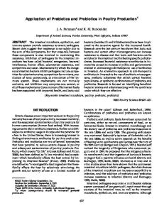
In this equation, X is the fractional conversion, G is the specific gasification rate, Mc is the molecular weight of carbon, and t is time. After plotting and analyzing the basic experiment (no additional catalyst at the above settings) they determined that the linearized form of the equation does in fact hold for the case. Next they explored different pressure and temperature conditions for the experimental setup. The result of the experiments is that they determined that lower pressures and higher temperatures greatly increased the gasification rates. The technical feasibility of poultry litter gasification is due to several factors, including the low pressures, quick equilibrium conversion, moisture content of the litter, potassium catalyst already contained (although more catalyst greatly speeds the reaction), and fact that the broiler litter contains less sulfur than coal, which is environmentally favorable. Because of this finding, they determined that it is technically feasible to gasify poultry litter, which led them to do an economic analysis. The system they proposed in their paper was a transportable gasification system, designed to be built on the trailer of a tractor-trailer, which can process 1.5 tons of broiler litter per hour. Their proposed system consists of a feed hopper, and reactors having a diameter of 1 meter, and a height of 2.3 meters, the litter being moved through the process by screw conveyers. A sketch of the system that the authors proposed is recreated below (Figure 2.1): The authors calculated the residence time of the above reactors as 180 minutes, for 4.5 tons. The reactors in question combine drying, pyrolysis, and steam gasification in one unit, with operating temperature of 700°C and 345kPa. The fuel gas produced by their reactor has a heating value of approximately 10,400 kJ/m3, with an approximate 630 m3 9

Knockout drums

Screw Conveyer

Compressor Feedstock Hopper

Moving bed gasifier

Heat Exchanger

Ash container Condensate Collector

Figure 2.1: Sheth and Jones’ Description of Transportable Gasification System

of fuel gas produced per hour. The value of the gas produced by their process, assuming a price of $2.75 per million Btu, was $17.06 per hour. The total investment of equipment would be $130,100, for the small transportable system they designed, and was meant to be mounted on a tractor trailer for transport to local farms. The work presented above was continued in the next journal article analyzed, which was entitled “Kinetics and Economics of Catalytic Steam Gasification of Broiler Litter” by Sheth and Turner [6]. In their study they continued to carry out basic kinetic and economic research on suitability of gasification of poultry litter for energy conversion. The main goal of their study was to further define and verify the kinetics for poultry litter catalytic gasification, and to develop a design for a larger stationary plant, with the economics of that plant. This study could be broken down in to two main parts: development of the kinetics equations for the catalytic steam gasification reaction, and their experimental verification, and the development of a technical and economic plant model. Below (Figure 2.2) is a recreation of the chart Turner and Sheth created to document the catalytic gasification process they designed for the poultry litter. It summarizes a catalytic gasification processing system, which as can be seen can be modified to include biomass of any form, including municipal solid waste, and includes two useful output streams, the low BTU gas, and ash for sale to the fertilizer or concrete industry.

10

Poultry/Animal Manure

Gasifier (1300-1500°F, 50-100 psi)

Biomass

Source of Additional Potassium

Solid Gas Separator

Low Btu gas

Steam Solids to fertilizer or concrete industry

Figure 2.2: Sheth and Turner’s Description of Large Scale Gasification System

For the technical portion of their study, the authors used extensive experimental data to derive a rate mechanism for the catalytic reaction. For the economic portion of their study, the authors assumed a fixed processing plant with a larger capability. They assumed the plant operates for 330 days a year processing 100 tons of poultry litter a day. They also assumed a 1350°F operating temperature and a 100 psig operating pressure and a 10wt% catalyst loading. They assumed for their study that the litter itself has a 3wt% loading of catalyst, which meant that 7wt% langbeinite would need to be mixed with the litter for proper catalysis. They assumed the litter cost to be $10 per ton, and the transportation costs to be $1 per ton. In estimating the cost of the plant they used the 6/10th factor and other scale up techniques. They ran their designs for a 500 tons/day operation, and a 1000 tons/day operation, with gas prices of $14.52 and $9.85 per million Btu, which were the sale prices during the 2000-2001 period. The char residue leftover from the gasification process was assumed to have a value of $29 per ton as fertilizer. However, the authors cite a newer study which states that the char fertilizer price could be as high as $50 to $85 per ton. As can be seen from their work, the greater the feed rate, the quicker the payback period. However, there is no comparison to real situation plant economics, so the model was not verified or validated. The overall recommendation was that the bigger the processing capacity and capability the better for the case of poultry litter gasification. From the available literature, it is apparent that catalytic steam gasification is a valid technological option for processing of biomass for energy, in the form of low BTU 11

heating gas. Economically it poses a viable case, and is among the most environmentally friendly options. The next area to be addressed is the application of a system to produce power directly from the gas produced by the catalytic gasification plant proposed. The implementation of an Integrated Gasification Combined Cycle is an area of much research by GE and other companies, and there are numerous publications on the subject.

2.4. Integrated Gasification Combined Cycle (IGCC) Directly tied to gasification of waste, the application of an IGCC is a topic that is coming to the forefront in power production alternatives. One of the biggest arguments in favor of the IGCC is the high level of efficiency that can be achieved, and this efficiency is going up all the time, with new technological advances and experience, all the while the installed cost per kilowatt is decreasing. For agricultural nations and areas with little fossil fuel availability, this is a very attractive option for sustained power generation. One of the more general, but very important papers on this subject is entitled “New Power Production Technologies: Various Options for Biomass and Cogeneration” by Kai Sipila [8]. This paper concentrates on the area of biomass utilization in a broader scope, and how it applies to power generation, covering the different fuels and applications. The author’s main line of argument in this work is the need for the development of biomass for energy production. He argues that renewable resources such as hay or grasses could provide a great deal of energy production, if the available unused land was put into production. With the growing power demands all over the world, but especially in third world countries, there is a real need for renewable power resources. He goes on to state that the use of biomass for fuels would additionally have an enormous impact on CO2 emissions, and the use of biomass derived fuel additives could reduce CO2 emissions from vehicles. Sipila’s discussion on biomass utilization in Europe cites an up to 14% of the national energy production is from biomass, achieved in Finland, with an additional 4% of their energy coming from peat moss. He proposes that this will see a sharp increase as the trend towards growing crops for non-traditional uses continues to expand.a Sipila closes by saying that biomass will continue to see a large amount of growth for energy production in Finland as well as the rest of Europe. He goes on to state that if biomass is more efficiently produced and utilized, there could be an additional 200-250 TWh/a (Terawatt-hours/annum (year)) of electricity produced. This would help significantly to meet the growing energy demands while simultaneously reducing harmful CO2 emissions. a

This can be readily seen in America as corn is becoming more and more highly utilized for ethanol production. According to the USDA 620 million bushels of corn were used for ethanol in 2000-2001.

12

Another article that closely mirrors the above work is “Cogeneration Based on Gasified Biomass – a Comparison of Concepts” by Fredrik Olsson [9]. This paper, published in the proceedings of the International Conference on Efficiency, Cost, Optimisation, Simulation and Environmental Aspects of Energy and Process Systems (2000: Enschede, Netherlands) focuses on the production of power from gasification of biomass, and the efficiencies possible from the use of the integrated gasification combined cycle (IGCC) and the integrated gasification humid air turbine cycle (IGHAT). Through careful simulation, the author calculated the electrical efficiency and fuel utilization for both of these systems. For the IGCC system, he found the electrical efficiency to be 45%, with fuel utilization of 78-94%, which is a measure of how much of the fuel was converted. For the IGHAT system, he found similar results; however, this was estimated under the assumption that combustion is possible in a highly humidified environment. The purpose of Olsson’s work on gasification of biomass as fuel for a turbine is due to the fact that solids, such as biomass, are not feasible as direct fuel sources for power generation in a gas turbine application. The reason for this is that solid fuels cannot be directly processed through a turbine, since solids cannot feasibly flow through the blades, compressor, and turbine workings. The solids must either be combusted to produce an indirectly heated gas (as in the case of an IFGT) or converted into another gaseous or liquid fuel source. This led to the development of gasification to produce a fuel gas that would be applicable in such a setting. The fuel that the author uses as his test case is forest residues, i.e. wood chips, bark, etc, with a moisture content of 50% and a LHV of 8.3MJ/kg. This fuel is dried, and then processed through the gasification system, with the fuel gas produced combusted in one of the two turbine cycles analyzed. The IGCC uses a pressurized gasification system and steam drying of the biomass. The air used in the gasifier is bled off of the turbine and compressed in two stages before entering the gasifier. The fuel gas produced is cooled, filtered, and combusted in the turbine, then the exhaust gas is passed through a heat exchanger to produce process steam. In the configurations that the author explored using gasification at near atmospheric conditions, work needed to compress the gas was saved, and the process was simplified, however, the gains were not as great, due to increased heat loss. In the HAT version, the exhaust waste gas heat is recycled back into the system. For the HAT, the main difference is that the heat recovery steam generator (HRSG) is replaced with a recuperator and economizer. One important note about this system is that there is only a 600kW natural gas fired version in operation, as this is a new technology that is relatively immature as a technology option. Whether it could even operate on the lower quality fuel gas produced by the gasification process is one of the issues that the author raises. The humid air turbine does pose a significant advantage over the compressed air option on the front of thermal efficiency, since it provides more heated steam with the same amount of work done by the turbine. Through Olsson’s research, the author determined that the IGCC could achieve electrical 13

efficiencies approaching 45% of the LHV for the fuel, when operated at higher pressures. This represents a 4-5% improvement over atmospheric systems of similar design. The reason for this is because there is no need for fuel gas compression since the gas production system, and entire upstream portion is already pressurized, and there is less heat loss in the gasifier and gas cleaning system from the lower pressures. In Olsson’s work, the author goes on to compare the electrical efficiencies for each of the options. From his analysis he determines that to reach the maximum efficiency for the IGCC, the pressure ratio of the turbine (the ratio between the inlet and the outlet) would have to be prohibitively high, however, the curve that describes electrical efficiency as compared to pressure ratio is mostly flat, so there is little disadvantage (~1-2%) to lowering the pressure ratio. In addition, he found that the steam dryer poses a slight advantage, about 1%, over the exhaust gas dryer. Regardless of which of these configurations are analyzed, both pose significant advantage over the more common turbine system used. The advantage over this system ranges between 5% and nearly 15%. The data for fuel utilization that the author presents paints a different story. From his analysis, he determined that the fuel utilization for the HAT cycle would be very low, due to the overabundance of water vapor in the exhaust gas. The abundance of water vapor causes a shift in the dew point which causes cooling issues, such as the water coming out of vapor phase and causing too much cooling to the surrounding environment before encountering the heat exchanger, this in turn lowers the overall efficiency. The calculated efficiencies of fuel utilization are between 78% and 94% according to Olsson’s analysis. This data is comparable with the more common turbine systems. Olsson concluded his analysis with several technical development points that needed to be addressed. First, with regards to the steam dryer, he cites corrosion and erosion problems at high temperatures and sometimes due to demanding chemical environments. Second, he cites difficulties in feeding the biomass feedstock into a pressurized gasifier. This poses a technical difficulty because of issues keeping the gasifier pressurized while still ingesting fuel. Thirdly, he points out the issues with tar cracking. If not cleaned from the fuel gas, tar from the biomass can accumulate in the heat exchanger. He states that using a second catalytic reactor, or tar specific catalytic material in the gasifier could take care of this issue. Finally, Olsson points out issues with NOx emissions. He cites several technologies that could deal with this technological hurdle, such as nickel catalysts, a rich-quench-lean combustor, or catalytic reduction. Another article more specific to the application of an IGCC to biomass based power generation is “IGCC - Clean Power Generation Alternative for Solid Fuels” by Norman Shilling and Dan Lee, both employees of GE [10]. In their study, published in PowerGen Asia, in 2003, the authors address the factors that contribute to the applicability of an integrated gasification combined cycle (IGCC) power system. The key criteria the authors cite for these factors are the environmental improvements over traditional 14

combustion based systems. Namely, reductions in ash and greenhouse gases are the primary enhancements to environmental impact. Given that these systems are a relatively new technology, there is a rapid advancement curve, which is driving costs down and technology and reliability up. The authors cite that GE gas turbines have 500,000 operating hours on synthetic fuels, and that GE is involved in more than 14 IGCC projects. These plants range from 40 to 550 MW in size, and have recorded availability numbers in excess of 90%. Environmentally, the authors cite IGCC as being the cleanest technology for dealing with solid fuels, with the least amount of pollutant byproducts. They cite the IGCC in addition as having the lowest production of NOx and SOx compounds. In real world application, the authors cite the plant at Polk County, Florida (Tampa) that has been continuously outperforming conventional plants for the past 6-7 years. NOx emissions are much lower due to the lower operating temperatures of the IGCC plant as opposed to the direct fired combustion plants. In order to approach the NOx emissions of a gasification plant, conventional plants must use selective catalytic reduction (SCR) to clean the flue gases. This is a potentially harmful process in itself as it requires the addition of large amounts of ammonia to the hot ash and flue gases for reaction to occur. The author claims that this renders the ashes unsuitable for further utilization or resale.b In addition, the design of the gasification system immobilizes many metals contained in the fuel, allowing them to be safely removed with the solid ash and not releasing them through the exhaust gases, while the medium volatility metals are removed during the synthetic gas cleaning process. Mercury also is much easier to deal with in a gasification system, as it tends to be chemically reduced in the gasification processing, allowing it to be treated by sulfonated activated carbon. This is a catalytic material that the flue gas flows through, chemically reducing the mercury with the sulfur and capturing it in the matrix, just like a common mercury spill cleanup kit. The authors cite this as being similar to the operation currently undertaken in the Eastman Chemical’s acetate plant at Kingsport, TN. Another key argument the authors make for IGCC systems is the wide range of fuel flexibility available. Not only have a wide variety of various fuels been gasified in IGCC systems, but if the syngas produced is of too low of a quality, there is always the option to co-fire the turbine with natural gas, as is common practice, to maintain electricity and heat production values. This fuel flexibility plays into the economics of the plant because it gives energy production operations a level of independence from fuel cost variations, which can be a make or break item for single source systems. The authors next covered the differences in combustor design required for the IGCC system. Because of the lower BTU values of produced syngas, the combustor has to handle five times more volume than a natural gas fired turbine, which after dilution brings the flow to eight times a standard system. The problems associated with noise, b

In reality, ammonia is a very commonly used in the chemical fertilizer industry and this ash fortified with ammonia could have a very strong sales market in the agricultural industry.

15

achieving full combustion of the high mass flow fuel, and temperature control led the authors to point out that further testing and refinements of the system are required. It is mentioned that a facility is being constructed in Greenville, South Carolina dedicated to the further testing of IGCC systems. Furthermore, Shilling and Lee go on to highlight the versatility of the turbines available for combustion of syngas. Not only are they able to effectively utilize the varying qualities and compositions of various synthetic gases produced from gasification processing, but these turbines are also able to handle different mixtures of diluents, and able to modify and optimize on the fly. Co-firing in particular comes to bear on this process, since it allows much flexibility to the energy generation process. They report values of the ratio of syngas to natural gas from 65/35% as the operational standard, all the way up to 90/10% for a plant operating in Singapore, owned by Exxon. Economics are another of the key areas that have been improved through technological development and optimization. The data presented in this paper show a decrease of nearly $1000/kW over the past 20 years, leaving the current cost per installed kW of $1200-$1400. In addition there has been much work done to integrate the processes, streamline efforts, and improve outputs that are determined to improve the economic viability even further. One of the key limitations is the ambient temperature of the intake air, or more specifically the density, which decreases rapidly as temperature increases. The authors cite a break point in the power generation due to the temperature of the ambient air, where higher temperatures above a point cause the turbine to limit airflow and decrease power generation. They cite that the Tampa Polk plant determined this point to be 90°F. However, there are several developments in the works that should help to extend this range significantly. Similar to the above discussion on commercial and industrial applications of the discussed technologies, the following section gives a real world anchor to the technological options presented. This is an important piece to understand when considering options and helps to answer the questions, what is this really going to cost and how well will this really work?

2.5. Municipal Solid Waste While municipal solid waste (MSW) might seem to be out of place as a topic for this work, it actually has a great degree of bearing on the application of energy production from biomass derived waste products. Commercial application of green energy production technology is an important basis to this study, and is precisely what Jim Schubert and Konrad Fichtner cover in their article, “Gasification/Cogeneration Using MSW Residuals and Biomass” [2]. This work, commissioned by the City of Edmonton, Alberta, Canada, revolved around the development of a municipal waste processing center. Jim Schubert and Konrad Fichtner announced the results of a study where they 16

compared available technologies for producing useful energy from waste products and processes. Edmonton has a highly advanced recycling and composting system, which leaves a large amount of solid, low density waste with high caloric values. The city had defined a goal of making waste processing a net zero or energy producing process, which led them to explore ways to produce energy from household non-recyclable waste. Producing energy from the waste has several benefits, including increasing the useable life of the landfill due to less space being taken up, producing energy for the waste plant and the city, and obtaining green and low emission credits for producing energy from renewable resources and lowering dependence on fossil fuels. Their study analyzed fluidized bed combustion (FBC), gasification, and pyrolysis for energy production, mostly in the effort for green power production. They identified three key companies that have current commercial energy production facilities using MSW. The first (and cheapest) alternative was provided by Enerkem, a Canadian company that uses a gasification approach. After the waste is gasified, the resultant gas is then processed through reciprocating engines to produce power. They state there is an operating plant in Spain that uses this technology. The second alternative, and next most expensive, was offered by WasteGen, which is based out of the UK. This alternative is based on pyrolysis, where the gas produced from a kiln is burnt to power a turbine and provide heat back to the pyrolysis kiln. They state that a plant using this technology has been in operation in Germany since 1987. The third option discussed, and the most expensive, was offered by the Swiss company Thermoselect. This option has the best efficiency, using both gasification and pyrolysis to greatly improve overall efficiency. However, they state that the plant built to use this technology had to shut down for economic reasons. The proposals that the city received varied from $7,000/kWhr for the Enerkem gasification system, to $14,000/kWhr for Eberra’s FBC and Thide’s pyrolysis system. c The total capital costs of these plants went as high as $212M for Thermoselect’s proposal. Through their cost breakdown, the city decided that Enerkem’s solution, using a gasification system, would be the best option, which has the distinct benefit of being the second cheapest alternative at $73M installed. All of these were reported in Canadian dollars, which at the time that their work was published, was trading at 1 to 1 with the US dollar. This work gives a benchmark on the applied work being done by other municipalities, and a data point for the scale of capital investment required for such an undertaking. However, these costs could be inflated, especially when compared to the literature from some of the other major companies in the field.

c

This installed cost is much higher than other published literature values, which give prices between $1,000-1400/kWhr for an installed IGCC system, which is stated as being higher than conventional combustion systems. (Shilling, 2003)

17

2.6. Environmental Considerations The final component of literature on the subject at hand that needs to be discussed is the environmental impact of the technology options. One of the major topics for discussion is the production of nitrogen species from combustion activities. In their paper “Investigation of Nitrogen-Bearing Species in Catalytic Steam Gasification of Poultry Litter”, Bagchi and Sheth investigate the nitrogen species produced through catalytic steam gasification of poultry litter [11]. There are several environmental issues that prompted this research, the resolution of which are required before steam gasification of poultry litter can hope to be a commercialized product. Chief among these concerns is the production of NOx. NOx emissions are a target of the EPA for reduction in both automobiles and factory emissions. In order to be considered an environmentally friendly option, any process must be able to prove that its NOx emissions are below harmful levels. Through a literature review and engineering analysis of the process, the author theorizes that the production of NOx is low, because steam gasification is at lower temperatures and is oxygen deprived (there is no air flowing through the chamber). Bagchi and Sheth then cited an experiment where water was left in the chamber to absorb whatever gases were emitted, and the pH of that water was actually higher, leading the researchers to believe that ammonia was produced instead of nitric acid. The key reactions involving nitrogen in catalytic gasification are outlined below: N 2 ( g ) 3H 2 ( g ) 2( N

X ) solid

2 NH 3 ( g )

N 2 (g)

X 2 (s)

(CEQ-9) (CEQ-10)

In the above equation, “(N-X) is the solid phase compounds of nitrogen present in the litter.” (Bagchi, 2005) The theoretical kinetics for the absorption of nitrogen into the dilute HCl solution is outlined below. dN kN (EQ-9&10) dt ln(1 X N ) kt In the above equations, N, represents Nitrogen content of the solid being gasified, k, is a first order rate constant, t is time, and XN is the fractional nitrogen conversion. Bagchi and Sheth demonstrated experimentally that the overwhelming majority of nitrogen was converted to ammonia, and that the kinetics for ammonia production are not first order, based on the experimental concentration data. These results are very important to catalytic gasification of biomass that has high nitrogen content. Because the majority of the nitrogen is converted to ammonia, there is 18

no need for expensive catalytic converters of NOx to control emissions. However, since there is a large amount of gaseous ammonia present in the hot flue gasses, there is a need for a wet scrubber or a simple condenser system to be included. This condenser would produce liquid ammonium hydroxide solution which could also be sold as a product, including as ammonia for the fertilizer industry. The lack of NOx gives catalytic steam gasification a definite advantage over the combustion based alternatives, especially with growing pressure to clean up pollutants from industry, and the possibilities for green credits for low emissions. 2.7. Economics The one thing that ties together all of the previously analyzed literature is an appropriate economic analysis. The underlying economics are what really drive the decision process to construct or implement any of these options. The purpose of these systems is to produce products for sale, whether that product is fuel, electricity or fertilizer. The technical developments are merely a means to an end. While Bianchi’s work summarizes much of the economics behind the combustion based alternatives (the IFGT and STC), the paper entitled “Preliminary Economic Analysis of Poultry Litter Gasification Option with a Simple Transportation Model” by Atul Sheth and Jennifer English covers much of the economic considerations behind a catalytic gasification plant [7]. This paper applies to the work at hand because of its thorough, although preliminary, economic analysis and its summary of gasification advances. The transportation model of the English and Sheth paper does not seem to apply to this work, as the biomass sources is assumed to be co-located with the energy plant. If this were not the case, their work could be immediately applied to determine the optimal distances to bring feedstock. The transportation model could apply to a degree to this economic model though, since the waste ash is planned to be sold and transported to either the concrete or fertilizer industry. In that case, the model would have to be greatly simplified, because the density of users would not be so much of a factor, since there are only expected to be a handful of purchasers. In their work, English and Sheth describe the catalytic gasification process, and equipment costs, as developed by Turner, Jones, and Sheth in their works. They then go on to elaborate on the economic model, developing present cost adjustments through the following equation: Pr esentCost

OriginalCost * (index@ present / index@ original)

(EQ-11)

The indexes in their work were obtained from a chemical engineering journal. From this development, the authors went on to develop the cost scale up equations using the equation: CA=CB*(SA/SB)0.6 19

(EQ-12)

In this equation, A and B are the same equipment, or similar equipment, but different size. CA is the cost of equipment A, CB is the cost of equipment B, SA is the size of equipment A, SB is the size of equipment B, and 0.6 is the scaling factor. The above equation (EQ-12) is known as the 6/10th scale up rule, taken from the work by Peters and Timmerhaus. This scale up rule allows the estimation of larger sized process equipment based on the known costs of the same but smaller equipment, or vice versa. This is simply a numerical estimation, and is not to be confused with actual costs from industry quotes. Armed with the above equations, the authors were able to extrapolate the original design of the plant to larger designs, and extend the pricing to the current market. Next, the authors used the U.S. Census data from 1997 to estimate the density of poultry houses. The model for transportation costs and economic viability developed in their work was based on the density of poultry houses, distance to travel, and cost of travel. It is apparent in this work that the litter is assumed to be loaded on the truck as part of the chicken farm’s responsibility, as no pickup or loading costs are estimated. From the density data, and number of plants within a radius of the proposed plant, the authors went on to derive the total distance to each house in the area, which was simplified to the below equation (EQ-13): TD

* P * (2 / 3 * R 3

R2

0.5 * R 11 / 6)

(EQ-13)

In the above equation, TD is the total distance to each plant, P is the density, and R is the maximum distance to be traveled to the plant. The model is based on an annular (doughnut) distance of travel from the plant. The authors then went on to specify cost correction equations to bring the out-year expenses and revenues back to current year dollars, in order to more accurately determine the present value (PV) of the plant. These equations are: z

PVcos t

( AC1 * (1 I ) z 1 ) /(1 i) z

(EQ-14)

( AP1 * (1 I ) z 1 ) /(1 i) z

(EQ-15)

1

z

PV profit 1

In the above equations, z is the time in years, AC is the annual cost in year one, AP is the annual profit in year one, I is the inflation factor, and i is the time value of money. Based on correspondence with local banks, the authors used 2.75% for inflation, and 6% for the time value of money. Annual operating costs for the model were taken from Turner and Sheth’s earlier work, and scaled up with an exponent of 0.25, per Peters and Timmerhaus’ work [16]. The authors also used the $10/ton cost of acquiring the poultry litter that was assumed in the 20

earlier work by Turner and Sheth. For determination of the annual revenues from the plant, the author used the work of Turner to determine that about 10% of the biomass would be converted to char ash for sale, with sale prices between $29/ton and $50 to $85/ton [6]. Due to preprocessing concerns, the author decided to stick with the $29/ton price. For fuel gas production, the author again cited Turner and Sheth’s work, which stated that for every ton of biomass; approximately 420m3 of gas is produced [6]. After evaluating these equations in a program written in Visual Basic 6©, the authors were able to produce charts estimating the costs and expenses associated with a plant of 100, 500, or 1,000 ton/day capacity, and determine the break even time and profitability of each option. In addition, they were able to vary the population density of chicken farms, and prices of products to achieve a sensitivity analysis on the various options. Through their work, the authors determined that the best option for the Tennessee area would be a 500 ton/day plant, due to the limited population density. The 100 ton/day plant would not be large enough to get the production necessary, and the 1,000 ton/day option would not be able to be supported by the local poultry industry. However, the authors point out that Batesville, AR, with its high density of poultry farms would be able to easily support this more economically viable solution. While the work conducted by English and Sheth utilizes a different feedstock, and requires pickup, purchase, and transport to the plant, the basics of the economic model will prove greatly important to the work at hand. This work will be used as a foundation for the economic development attempted in this work.

2.8. Conclusions In the literature survey summarized above, we covered the main areas of research from published works that touch on our research. The technical developments published in the papers on the IFGT’s, STC’s, catalytic steam gasification, and IGCC’s were used to establish the four options pursued in our work. The support work published in the fields of environmental effects and plant economics were used to establish the feasibility for each case analyzed in our work. Finally, the work published on the municipal solid waste processing facility gave us a real world data point for a similar facility [2]. Together, all of these works from the literature survey form the framework around which our analysis of alternatives was built. Furthermore, the data from these works and others form the data points for the economic model that was built for this work. The complete and accurate research that was conducted by the scientists mentioned above is what made this work possible, and makes possible the future development of biomass based energy production systems. 21

CHAPTER 3. TECHNICAL ANALYSIS

3.1. Introduction In this section, the technical details of the energy production alternatives will be analyzed. These solutions will be grouped by type of system. First, the combined heat and power system concept will be analyzed, since this concept for energy conservation is part of all of the concepts analyzed. The energy efficiency improvement of a system that incorporates a combined heat and power cycle is great enough to make even borderline cases for power generation economically viable. After covering the technical detail of the combined heat and power cycle, we will cover the combustion based power generation alternatives. These options, the IFGT and STC, will be covered first because they are the most widely used technical option for energy production from biomass. Next, catalytic steam gasification and the IGCC will be analyzed from a technical perspective, because these two options go hand in hand as well. An IGCC is simply an electrical power generation unit such as a turbine or other engine combined with a gasification system to immediately utilize the fuel gas produced. In this section of this work, we will analyze the alternatives from a technical perspective, such as how they work, what are the characteristics and possible designs of such a system and what are the drawbacks. The information used in this analysis is drawn from the literature discussed in the previous chapter, as well as from other sources.

3.2. CHP Systems-Introduction and Background Combined heat and power (CHP) systems are the one common thread through each of the explored processing options. The capture and reuse of the waste energy from the energy processing, such as recovery of heat from flue gasses, is the key to optimizing any energy production process. The application of a CHP is integral to improving the efficiency of the IFGT, STC, and IGCC. CHP systems can reach efficiency levels of 55-60%, and have even been reported to achieve efficiencies of up to 90% [12]. These levels are the overall energy efficiency of the system, which includes both the thermal and electrical efficiency per energy input. For this reason, it is important to spend time explaining its technical aspects and importance. The CHP system can be summarized as a system that captures waste heat from an energy production process for other heating or cooling uses. Through the capture and utilization of waste energy, the overall energy efficiency of a system can be greatly improved. When energy is produced from combustion or another high enthalpy process, the waste gas streams exit the system with a large quantity of the potential heat that was produced. 22

Traditional System

Output

CHP System

Electric Generator

X MW & Y lbs steam

CHP - (Electric Generation & Flue Gas Heat Extraction)

Boiler (Steam/Heat Production)

Figure 3.1: Combined Heat and Power Concept

By installing a heat exchanger in line with this waste stream, the capture of the waste energy is possible. These systems can then be used to sell either hot or cold utilities to a customer. The distance from the plant that this is feasible for would have to be calculated, due to energy loses from underground piping. A simple schematic of a CHP system is represented in Figure 3.1: Figure 3.1, shown above, demonstrates the reason behind the large energy savings that can be achieved and used to make steam in a CHP system. If heat is extracted from the flue gasses, instead of using a separate boiler system to provide steam heating utilities, the costs required for energy production can be greatly enhanced, and the energy efficiency gains through utilizing that “waste” heat can be very large. Instead of dealing with energy efficiencies and losses from two separate systems, only one system is used, and the heat that is harnessed was formerly waste. In future energy system designs, as well as retrofits of current energy systems, conservation techniques such as CHP must be incorporated as a core technology in order to ensure a successful program. With rising energy costs and decreasing natural resources, we are now dealing in the margins that we used to consider waste. Even small margins of improvement in a system can yield great gains over its lifecycle. Operations and maintenance expenses can account for the majority of the system total lifecycle cost, so incorporating these into any analysis is a major component. CHP systems are incorporated into both of the options outlined in the following chapters, and are a key part of the analysis process. These systems enable efficiencies that make 23

fielding biomass fuel based systems economically feasible, and even attractive. For the fluidized bed combustor case, both the indirectly fired gas turbine (IFGT) and the steam cycle (STC) designs, CHP is incorporated through the recovery of heat from flue gases with the IFGT, and from recovery of the steam from the steam cycle. Through these energy savings measures the efficiency is greatly boosted. For the case of gasification, an integrated gasification combined cycle (IGCC) is the option analyzed in the present work in lieu of selling the produced gas. There is much work on this subject, mainly dealing with IGCC plants that run off of coal. IGCC plants are cited as reaching efficiencies approaching 45%, and with technological advances are expected to push even higher [10]. One major technological hurdle to overcome with combined heat and power systems is the distribution of the heating utility. Due to thermal loses, even insulated piping can only distribute steam or heated water to a limited geographic area. With current technologies, the heat utilized would need to be analyzed for effective distribution area. This will be a factor of steam/hot utility production quantities and heat losses to the environment over the run of piping. The hot utility produced could be a valuable asset in cold environments due to the large expenses incurred for heating, especially with rising natural gas and heating oil prices. In areas such as New York, with high electric, fuel oil, and natural gas prices, this would be a large economic advantage, if an effective distribution network could be established for the heating utility produced. An additional problem is that the heated water produced is of relatively low temperature, 120-140°F [8], which is not enough for many applications. This could be used for residential radiant heating to a degree, especially if the proliferation of radiant floor heat is increased. The most likely option however is the production of “pre-heated” water for other utility uses. The cost of raising 140°F water to high temp steam is much less than the cost of raising 70°F or lower water to steam. Combined heat and power systems are becoming a core technology for future power generation systems. Both conventional and biomass based plants are increasingly looking to this technology to increase efficiency and enhance the plant economics. Indeed, it is fast becoming the standard for new system design, especially due to the enormous savings it poses in pollutant productions. In the next section, we will analyze the primary set of systems that utilize this CHP technology, the combustion based alternatives. The two primary combustion based alternatives analyzed in this paper are the IFGT and STC. These two options will be primarily analyzed because of the wealth of data on the systems and the technological development that has already been put into these two alternatives.

24

3.3. Technical Analysis of IFGT & STC Systems 3.3.1. Introduction In this section, the two combustion based alternatives will be explored. These two alternatives, the IFGT and the STC were researched extensively by Bianchi et al in their work with our specific biomass, poultry waste including meat, feathers, gut waste, and bones. One thing to note is that the waste fraction from cleaning the poultry is mainly feed/litter from the gut. This biomass is more similar in nature to the poultry litter analyzed in the gasification system. However, the research from Bianchi’s group was on poultry waste feedstock, so it can be assumed that this would include a fraction of the digestive waste. Combustion of biomass to produce energy through a turbine is probably the most straightforward and easily understood and commercially developed approach to energy production. This process is widely used worldwide, with fuels from coal to wood pulp. The most likely design option for combustion is a moving bed combustor coupled with a turbine; this is commonly referred to as an indirectly fired gas turbine. An indirectly fired gas turbine (IFGT) is a mature, well developed approach for producing energy from solid waste materials. This option provides the greatest versatility, maintainability, and sustainability due to its well developed technology, well understood mechanisms, and base of support domestically. In addition, turbine technology is very scalable, which allows a great degree of flexibility in fuel sources, as other items are discovered that can be processed for energy production, i.e. municipal solid waste (MSW). An IFGT receives its name from the indirect method of heating the compressed gas. In a regular gas turbine, fuel is mixed with the air in an internal combuster, and burned, providing gas for the turbine (the fuel is usually natural gas or some other light fuel). This works well when there is a clean fuel that will not gum or foul the moving parts internal to the turbine. The externally or indirectly fired gas turbine however, is excellent for applications where solids such as coal, or other materials that either cannot physically be mixed in the gas moving through the turbine, or cannot move through the turbine due to fouling of the moving parts. In this application a moving fluidized bed external to the turbine heats the compressed gas, which is then expanded through the turbine blades. The application to the processing of poultry waste byproducts by means of an IFGT is well discussed in the work by Bianchi [3], where they did a thorough computer modeling and analysis to determine the ideal design of an IFGT for this process. In this work, Bianchi used a chicken plant that produced 35,000 tons of chicken waste a year (95 tons/day assuming 365 day service), and designed an energy production process based on this waste. Rather than reinvent the wheel, their comprehensive design and analysis will 25

be used as the basis for the IFGT analysis in this study. 3.3.2. Technical Discussion 1.1.1.1 IFGT Technical Analysis In this section the technical details of an indirectly fired gas turbine will be analyzed, from preprocessing of the poultry meal to scrubbing and heat recovery of the exhaust gases. For the majority of this section, the work of Bianchi et al [3] will be relied on due to the detailed analysis that they undertook, and its direct applicability to the problem at hand. Details such as biomass throughput rate and other design criteria will have to be analyzed and adjusted for the specifics of the location of this project. According to our literature survey, all of the technologies considered require preprocessing of the biomass for proper combustion. Primarily the particle size must be decreased and surface area must be increased for a greater degree of combustion. Typically this is accomplished through cooking, combining the feathers with the bone/meat, drying and grinding to a meal consistency. This meal must be dried from 70% (by weight), which is the as received moisture composition, to around a 12% (weight) composition of moisture. This could be easily accomplished through steam treatment, and from the paper by Bianchi et al, they stated that a steam utility at 180°F which would be sufficient for drying the meal to the required consistency for combustion [3]. The cost of the heat utility is addressed in the economics section, and the energy required for drying is addressed in Table 3.2. As stated before, all technology associated with this option has been fully developed and is in commercial use at many sites around the world. However, optimization for this fuel (poultry processing waste, meat, feathers, bones, gut waste) is a design requirement for this option. In an Italian study, published in Energy in 2006, M. Bianchi et al [3], did just that. In their study their group did research, modeling, and analysis to optimize an indirectly fired gas turbine for combustion of feathers, meat, and bone which were waste from a chicken plant. They used the waste tonnage from the plant, 35,000 tons per year, as their usable biomass for the study. In Bianchi’s modeling efforts, the author compared several different configurations of turbine system to find the ideal one. The configurations that the researchers analyzed were different compressor ratios, which is the ratio of the inlet pressure to the outlet pressure. This factor is the main determinant of the power generated by the turbine and plays a central role in cycle efficiency. The authors then compared power outputs and costs for burning just the feathers, meat and bone, to the power and costs of burning the aforementioned along with the recovered chicken oils, instead of removing those from the process and selling them separately. The team also compared a compressed air turbine to a steam cycle turbine, and different configurations of those designs in their 26

Table 3.1: IFGT Biomass Composition Composition H O N C S Ash

Unit wt% wt% wt% wt% wt% wt%

Inlet Meat 8 14.5 6.3 54.5 1 15.7

Inlet Feathers 6.4 27.8 12.5 40 3.3 10

Outlet Meal 6.6 17.2 9.7 46.2 1.5 18.8

Outlet Oil 10.5 9.5 0 70 0 10

(From [3]) work. In the introduction to Bianchi’s work on IFGT optimization, they cite the impetus for energy cogeneration based on poultry processing byproducts as both economic and environmental policy derived. Due to laws to prevent “mad cow” or other diseases, much of the market for poultry waste products seems to be in jeopardy. The disposal costs for the enormous tonnage of poultry waste produced every year from these endeavors is a large factor in the economic viability of energy recovery processes. In fact, in the conclusions of the Bianchi et al study, the energy prices and disposal costs are cited as being the two key variables and drivers to his economic analysis. In order to effectively discuss the work of Bianchi et al, the following sections of this work will discuss the sections of this study at length relate the results to our case, an IFGT located in Chattanooga, Tennessee. Rendering and Biomass Makeup: For their project Bianchi et al considered a plant which handles 35,000 tons per year of poultry industry wastes. In Table 3.1, is a recreation of the table in which they give the chemical composition of each poultry waste product they planned to handle. The above data presents very important information for this study, because the chemical makeup, especially the carbon content, of the biomass is a crucial data point. This carbon content will be later used to analyze the data from the catalytic steam gasification options since the authors of those studies used poultry litter as their biomass. The process that Bianchi et al designed for preprocessing of the biomass, which was outlined above, is summarized in Table 3.2. Some of the key specifications are the mass flow rates and power requirements. As can be seen, the cooker and dryer have quite large power requirements. Another note on Table 3.2 is that the authors calculated that the energy produced from the plant would be enough to run the cooker and other utilities, as well as produce energy for sale. The most efficient way to produce these heat utilities would be through the use of a CHP sequenced with the IFGT. Bianchi et al mentioned that the energy produced by the IFGT would be more than enough to provide the required heating utilities.

27

Table 3.2: IFGT Process Mass Flow/Thermal Specifications Rendering Process Main Specifications Inlet/outlet mass flow rates Inlet meat mass flow Inlet feather mass flow Outlet meat meal dry mass flow Outlet feather meal dry mass flow Outlet oil mass flow

2.25 kg/s 1.04 kg/s 0.45 kg/s 0.35 kg/s 0.21 kg/s

Thermal utilities specifications Thermal power to the cooker Thermal power to the hydrolyser Thermal power to the dryer Steam temperature to the cooker Steam temperature to the hydrolyser Steam temperature to the dryer

1.2 MW 0.76 MW 0.95 MW 180 C 140 C 180 C

(From [3])

The downstream part of the design studied by Bianchi et al was a rendering process, which was combined with a fluidized bed combustor and IFGT with CHP heat reutilization, to make up the total process they simulated for the given mass flow rates (Table 3.2). Through this simulation the authors determined the required size of the heat exchanger, ideal pressure ratios for the turbine, and overall electrical, natural gas, and total efficiency based on the varied combinations they explored. The schematic of the system they proposed and analyzed in their paper is recreated in Figure 3.2. This schematic includes the hydrolyzer for the feathers, the dryer, cooker, IFGT and heat exchanger. The hydrolyzer is a piece of equipment that breaks down the feathers using steam into proteins that are more easily processed. It is important to note that this schematic is only Bianchi et al’s proposal for an energy plant at their location, and this layout would need to be tailored significantly for utilization at the Chattanooga, Tennessee location. The pre-processing units are of questionable utility, such as the cooking process, and the possibility of grinding and drying alone could meet the intent of pre-processing the biomass. The exclusion of the cooker could also enable the utilization of biomass besides poultry material. Layout and Configuration: The key design point of the above diagram is that the heart of the system is the fluidized bed combustor. The biomass is preprocessed in the cooker, grinder, hydrolyser, and dryer, and then fed into the FBC. The FBC is the heart of the system however, because it is the system that heats the gas for the turbine, and also provides heat to the steam generator for the preprocessing activities.

28

Feathers

Steam Generator 2

Steam Generator 1

Meat/bone

Hydrolyzer

Grinder Cooker

Dryer

Water Fluidized Bed Combustor Air

Compressor

Ash

Turbine

Feathers

Electricity Air

Figure 3.2: IFGT Schematic

The path of the gases (air is the working medium for this model) is the air after intake is compressed by the compressor and then heated up by the FBC to the inlet temperature for the turbine. The work from this compressed air is then extracted through the turbine and the excess heat is recovered by the heat exchanger. After passing through the turbine and out the diffuser, the authors then had the hot flue gases recycled through the FBC. These flue gases serve to maintain the temperature of the combustor at 800-830°C, which they state is the required value for that type of combustor [3]. Their plan for recycling the hot flue gases to keep the combustor going is brilliant because it internally supplies much of the necessary heat to keep combustion going. Energy recycling is a key point to the design laid out by Bianchi’s group. The excess heat from the turbine and fluidized bed combustor is used to heat the steam for the steam generators. The steam generators in turn feed hot process steam to the dryer, hydrolyser, and cooker. Through their thermodynamic simulations they determined that the heat provided would be sufficient to maintain process heating in addition to supplying power. [3] 29

These conditions for design are the general conditions that are pursued for many of the FBC designs with CHP, and would need to be optimized for implementation at the location of the plant in question in this research effort. In particular, the steam temperatures required, the ambient conditions of the plant, and the construction and design of the individual unit equipment would have to be taken into account. As stated before, research would be necessary to determine if the cooker and hydrolyser are even necessary, when drying alone could allow the biomass to reach a combustible state. Additionally, the plant layout would need to be designed to utilize other sources of biomass, such as bulk corn residuals, MSW, etc, in order to be economically viable across a variety of fuel source prices. Next, Bianchi used their proposed design to run a mathematical simulation to determine the key values for efficiency, pressure ratio, etc, which was in turn used to determine the plant economics. Some of the key assumptions that the authors made in their simulations of the design configuration are found in Table 3.3. Some of the factors that could have a large effect on the outcome of the model are the efficiencies assumed for the recuperator and combustion. Depending on particle size, water content, etc, the combustion efficiency could be greatly affected. Also, depending on heat exchanger design, the efficiency of producing the hot utility water could be modified greatly. The recuperator effectiveness was established in a pair of studies cited in Bianchi et al’s paper by “Langerstrom and Xie and Proeschel” [3]. In addition, if “dirty” process water is used, the composition of the water and its thermodynamic properties could be greatly altered over the ideal case assumption. Also, given the

Table 3.3 IFGT Simulation Inputs and Assumptions Assumptions for calculation Ambient air temperature Ambient air humidity Turbine inlet temperature Compressor efficiency Turbine efficiency Natural gas combustor efficiency Biomass combustor efficiency Recuperator inlet hot gasses temperature Recuperator effectiveness Compressor inlet pressure loss Gas pressure loss across steam generators Recuperator pressure drop FBC gas pressure drop Pressure drop at the stack Water inlet temperature at SG1

(From [3]) 30

15°C 60% 1150°C 0.87 0.87 0.99 0.95 750°C 0.9 2% 2% 2% 2% 2% 15°C

moderate climate of Tennessee, the temperature of the water at inlet could greatly vary depending on time of year, source, etc. The two major scenarios that they investigated are combustion of just meat and feathers, and combustion of meat, feathers, and oils. Two of their economic scenarios involved separating and selling the oil to other companies versus burning it for energy. IFGT-A is the scenario where only meat and feathers were burnt, and IFGT-B is the scenario where the oils were burnt as well. Bianchi first explored the effect of pressure ratio across the turbine on overall efficiency and created a chart that showed the data from their simulations to this end. Their chart showed two curves following mostly the same trend. Scenario B, with more biomass being combusted had a higher compressor ratio (pressure ratio across the compressor), due to the increased airflow required, and produced more energy. This trend was expected, since the only variable modified is the amount and type of fuel. The oils have a much higher lower heating value (LHV) than the meat and feathers, and therefore burn and provide energy much more effectively. The oils produced are certainly the preferred fuel from a technological standpoint, if not an economic one. Also in their work they demonstrated that the natural gas consumption of the IFGT follows the same trend, with slightly greater consumption with greater biomass utilization. Bianchi also explored the steam generation outlet temperature and the recovery temperatures were compared to the power of the generator. Their comparison showed the amount of steam utility that can be produced, or the amount of heat utility that can be recovered from the hot flue gasses depending on the size of the IFGT used. The data that Bianchi et al generated is very important to the operation of their plant design, because of the amount of energy required by the cooker, hydrolyser, and dryer. If the energy required to run those operations was procured independently from the plant’s own energy production system, the cost for the additional energy requirements could be prohibitive. Our work plays into the economic analysis of this alternative, because the key economic advantage of a CHP system is the utilization of not just the electric power generated, but the heat utilities produced. From this view of the analysis completed by Bianchi, it can be seen that with greater power production, the temperature of the additional utilities is reduced, leveling off around 325 to 350 Celsius. These temperatures are important for the design of the heat exchangers and heat recovery devices, as there are design thresholds for the utility steam and heat losses in piping between plants that must be taken into account. In addition, in the equations 16 and 17 below [3] it can be seen that power generation also increases with greater biomass utilization, which makes sense, more fuel, and more air, 31

produces more power. These equations are the core of the temperature and efficiency simulations that Bianchi conducted. Pel el

th

m NG

LHV NG

mbio

LHV bio

m NG

QCK QHY QFD LHV NG mbio LHV bio

(EQ-16)

(EQ-17)

In equation 16, P is the electrical power, ηel is the electrical power generation efficiency, mNG is the mass of natural gas, LHVNG is the lower heating value of the natural gas, LHVbio is the lower heating value of the biomass, and mbio is the mass of biomass. In equation 17 nth is the thermal efficiency, QCK is the heat needed by the cooker, QHY is the heat needed by the hydrolyser, and QFD is the heat needed by the dryer. From these equations it can be seen that the electric or thermal efficiency is mostly a function of the power or heat produced by the system, since the LHV is fixed. Gains in the efficiency of the system come from gains in either the heat production (heat transferred to the user systems) or the electric power generated from the turbines. [3] Bianchi et al showed that the efficiency goes up with power production, which is to be expected. They also summarized that “total efficiency rises with a decrease of pressure ratio, even if the mass flow rate increases, because of the predominance of the electric power increase” [3]. This is evidenced from the equations shown above. The efficiency peaks at 37%, which is equivalent regardless of which scenario of biomass utilization is chosen. The advantage is that scenario B provides an extra 20MW of power over scenario A at the lowest pressure ratio. Both scenarios follow mostly the same efficiency trend across pressure ratios and electric power production, with scenario A slightly edging B out in efficiency. From this information it can be seen that the efficiency of power production can be greatly increased with greater magnitude of mass flow rate. The economy of scale that says that construction of a large plant is more profitable also turns out to apply to the technical efficiency of the plant. Bianchi et al point out that the efficiency numbers do not necessarily paint the complete picture, as they take into account the biomass energy utilization in addition to the natural gas energy utilization. They argue that the correct way to optimize the scenario would be to find the maximum efficiency based on the natural gas efficiency alone, because that is the scarce and costly resource. They cite that equation 18 is the one that should be used when developing an optimization scenario:

NG

m NG

Pel LHV NG

32

(EQ-18)

In this equation, ηNG is the efficiency of natural gas usage, Pel is the electrical power generated, mNG is the mass of natural gas used, and LHVNG is the lower heating value of that natural gas. If this avenue is pursued, Bianchi et al charted the efficiency of the IFGT based on natural gas consumption. Bianchi et al stated that the natural gas efficiency peaks at around 51.5% regardless of system approach. The maximum efficiency is at a pressure ratio of 13, and efficiency decreases suddenly on either side of this value. In fact, the lower pressure ratios cause the efficiency to fall off more rapidly than do the higher pressure ratios. However, the difference between a pressure ratio of 8 and a pressure ratio of 13 is an efficiency difference of 2.5%, which may or may not prove to be significant. This analysis of the peak natural gas efficiency, led to the analysis of the steam cycle option (STC). The authors determined that the cost of natural gas is the long pole in their design tent, and rightly so, given the volatility of the fossil fuels market and cost of the co-firing fuel. Steam cycle plants have the advantage of not relying on natural gas as heavily because there is no additional boiler for steam production needed for peripheral equipment. The drawback to this however, is that they are not as scalable as the compressed air options. If one wanted to produce more power, with an IFGT you could simply co-fire with more natural gas and increase the turbine output, up to the design limitations. 1.1.1.2 STC Technical Analysis The steam cycle is the alternative type of power generation scheme to the IFGT. The steam cycle is very similar to the IFGT, in that it utilizes the same fluidized bed combustor. The main difference between the IFGT and the STC is that the working fluid is steam instead of compressed air. The steam cycle offers several advantages over the IFGT option, but mostly it offers advantage in the lack of reliance on natural gas. This is because the steam cycle version uses steam as the working fluid, it does not require a separate boiler for other options. For the steam cycle that Bianchi et al chose to analyze they chose a “condensing steam cycle” due to the low temperatures and pressures that the utilities that are being fed with leftover steam require [3]. This system would use biomass combustion to heat the steam, some of which is extracted for the different processes. The combustor temperature was set slightly higher in this scenario (900°C), and the exit gas was “limited to 240°C”. [3] The team cited that they used GateCycle© (a thermodynamic analysis software package) to run the numerical simulations of this type of turbine, to make the power production predictions. They named the two steam cycle simulations C and D, where the first cycle delivers steam to the turbine at 40 bars and 520°C, and the second cycle provides turbine steam at 11 bars and 320°C. They say that the second cycle is an attempt to find a solution that could meet peripheral utility steam demands but keep the cost of equipment 33

Table 3.4: STC Inputs and Assumptions Steam Maximum Temperature Steam Maximum Pressure First Extraction Pressure Second Extraction Pressure Deaerator Pressure Condensing Pressure Isentropic Expansion Efficiency Pressure Losses at Heat-Exchangers Stack Temperature

°C bar bar bar bar bar

°C

STC-C 520 40 11 4 1.6 0.05 0.85 2% 130

STC-D 320 11 4 1.6 0.05 0.82 2% 130

(From [3])

low, due to the much lower pressure and temperature needs. The interesting thing about the steam cycle that they analyze is that there are no fossil fuels incorporated in their design, i.e. no natural gas, as was used and analyzed in the IFGT. This option has the potential to provide large savings over the life of the system, due to the volatile nature of fossil fuel prices. The steam cycle plant is similar in peripheral equipment to the IFGT option, however, the energy and steam production systems themselves are very different, and require different equipment and different equipment sizing. The steam working medium is recycled directly from the low side of the turbine through the steam generators, providing additional heat for the combustor in addition to heating the cooker, hydrolyser, and dryer. The inputs to their analysis of the steam cycle are reproduced in Table 3.4. The above numbers are the assumptions and inputs that Bianchi’s group used for their model of the steam cycle option. Note the much reduced maximum temperature and pressure of STC-D. In Table 3.5, the results from their analysis are summarized. The efficiencies were calculated with the assumed operating temperatures and pressures for the above given range of data. In Table 3.5 below, the electrical efficiency and thermal efficiency are both defined because it is a CHP system, which means that the thermal efficiency plays into the overall efficiency of the system, since flue heat is not wasted. The thermal efficiency plays into the STC system since its design utilized the steam working fluid to run process utilities elsewhere (hydrolyser, cooker, etc). A couple of points to note for the steam cycles that Bianchi analyzed: the thermal efficiency did not differ for either configuration C or D, and the electric efficiency is very low for this type of system. For efficiency this low, the cost of fossil fuels will have to increase greatly to make up for the increased amount of biomass necessary to produce power. In particular, configuration D is less than half as efficient as the regular compressor system. 34

Table 3.5: STC Simulation Results Electric Power Electric Efficiency Thermal Efficiency

MW % %

STC-C 5.2 23.9 13.4

STC-D 3.8 17.4 13.4

(From [3])

Bianchi et al summarized the comparison between the STC and IFGT in the following analysis. To analyze the relative efficiencies of the two configurations of a CHP plant, and compare them to each other and to a regular power plant that has separate electric and heat generation components, the authors used the Energy Savings Index (ESI) calculations from Bhargava et al (EQ-19) [3]. ESI is a way of calculating the relative energy savings based on a reference value. This calculation is handy for alternative energy designs, because it gives a standard way to compare the efficiency of an alternative design to the already known efficiency of a standard configuration power production facility.

ESI

1

1 el * el

(EQ-19) th * th

Through equation 19 above, the authors were able to make this comparison. In the previous equation the (*) variables are the values for the reference utilities, where ηel is the electrical efficiency, ηel* is the reference electrical efficiency, ηth is the thermal efficiency, and ηth* is the reference thermal efficiency. The reference efficiency that the authors used in their study was from a weighted value for the reference values, defined by their proceedings from an Italian energy conference [3]: * el

* el , NG

* FNG FNG

* el ,bio

Fbio

* Fbio

(EQ-20)

This equation provides a weighted value of the electrical efficiency, providing a means of comparison from the reference point. In the above equation, the η terms are the efficiencies, and the F terms are the fractions of natural gas (NG) and biomass (bio). This equation allowed a reference base to be calculated for comparison to the values calculated for the plant design. The results of their computer simulations with regards to efficiency of each design, in terms of electric efficiency versus energy savings index (ESI) were then calculated. There are some key points from this analysis and their comparative simulations. First, steam cycle configuration D is less efficient than having the standard power plant with 35

Table 3.6: ESI Results (IFGT-STC Comparison) Plant IFGT-A max ESI (β=6) IFGT-A @ η (NG) max ESI (β=13) IFGT-B max ESI (β=6) IFGT-B @ η (NG) max ESI (β=13) STC-C STC-D

ESI 0.137 0.07 0.131 0.057 0.049 -0.234

(From [3])

separate electric production and heating. Steam cycle configuration C is slightly more efficient than the standard power/steam generation unit, but IFGT configurations A&B are the most efficient. The specific efficiency values required by the IFGT plants are 0.28 for A and 0.29 for B, in order to be more efficient than the baseline. IFGT-A provides slightly better ESI than B across the ranges of plant efficiency, as could be seen in their work. However, it is important to remember that B, while slightly less efficient than option A, has a much greater power production potential. The below recreation of the table by Bianchi (Table 3.6) summarizes the key points of their graph. In Table 3.6 above, the max ESI’s are given for IFGT-A and B, with β being the compressor pressure ratio at which this point occurred. For both of these models, the max ESI occurs at a pressure ratio of 6. In addition, the ESI was calculated for the maximum natural gas efficiency (η (NG)), which in both cases occurred at a pressure ratio of 13. The negative value seem for STC-D means that this plant design configuration was actually less efficient than the reference plant model. As can be seen above (Table 2.6), STC C has a similar value of ESI to IFGT A and B, when they are optimized for natural gas efficiency, only slightly beating out the reference plant configuration. At 0.137 and 0.131, IFGT configurations A and B beat the standard plant configuration by over 13%, which can be a huge savings for a large energy production scheme. Through the simulations by Bianchi et al of different pressure ratios they determined that the ideal IFGT would be one operated burning all available material (meat, feathers, and oil) instead of burning the meat and feathers and selling the oil. Three of the configurations that the authors of that study simulated would provide benefits over and above that of a standard plant configuration, with separate electric generation and heat utility generation units. However, they determined that IFGT-B would provide greater power production potential, with practically the same efficiency as IFGT-B. In the following sections the economics of this decision will be verified.

36

1.1.1.3 Environmental Analysis Environmental issues encompass solid wastes, as well as air wastes, and the potential for water pollution, given the proximity to the Tennessee River. There are some groups that are in violent opposition to combustion of waste for energy, although these groups are generally more in opposition to landfill waste being combusted, due to the heavy metals and sometimes toxic gases that can be produced from such activities. The main threats from combustion are greenhouse gases, nitrates, and sulfur containing compounds. The solid waste could be thought of as a profitable endeavor, since it could be sold as a fertilizer, given its high nitrogen content. One problem, which encompasses both alternatives, is the possibility of contamination of water supplies/personnel through E. coli or salmonella. Countermeasures to this type of environmental contamination of personnel or equipment would be similar to the ones already employed by the poultry processing facility. 1.1.1.4 IFGT & STC Conclusion For the economic conditions of the Chattanooga area, the steam cycle plant is favorable from a technical point of view because of its efficiency and lack of reliance on natural gas. In the above section, the design and optimization of both an IFGT and an STC were seen. Both of these designs by Bianchi showed the technical feasibility of an application of either system to combustion of poultry byproducts.

3.4. Technical Analysis of Catalytic Steam Gasification and IGCC 3.4.3. Introduction Gasification of the poultry waste is another strong alternative for energy generation. Through this process the poultry waste is converted to a low BTU gas plus energy, which can be either transported for other uses, or immediately combusted for electricity or heat generation. This is a “green” fuels process, as it can be used to make low BTU combustible fuel for use by other systems, in the form of methane or syn-gas. This gas could also be used as a feedstock for chemical processes. The primary employment of catalytic steam gasification of biomass is for use with a combined heat and power system in conjunction with the gasification system. This energy production alternative is an attractive one due to the possibility of getting transportable gas, in addition to having a heat and electricity utility for local utilization. Gasification applications in CHP systems were explored in the paper by Fredrik Olsson, “Cogeneration Based on Gasified Biomass - a Comparison of Concepts” in the ECOS 2000 proceedings [9]. These systems provide 37

a valuable alternative to combustion based systems. With gasification systems, there are none of the fouling issues that occur with combustion systems, which can be clumsy depending on the biomass being consumed. With poultry litter in particular this is an issue [5] and it is expected that this could be extended to poultry meal as well, given the similarities in composition. Catalytic steam gasification in particular was chosen because of its higher reaction rates, which means higher profits in a large commercial application. Given the large amounts of poultry waste that will be used in this system, any advantages in efficiency will pay large dividends in the long run. The purpose of this section is to draw on the knowledge base in literature of catalytic steam gasification and analyze the technical data which will support a decision for implementation in Chattanooga Tennessee. Catalytic steam gasification of carbon based material was developed by Exxon for gasification of coal, but later studies determined that there was application to biomass, including studies conducted by Hauserman [4] where he gasified poplar wood pulp. Sheth and Turner state that 1000 birds will produce 1 ton of litter per year [6]. They go on to cite a previous effort undertaken by other researchers to produce biogas from poultry litter using anaerobic fermentation as well as other combinations of techniques, all with only lackluster success. All of those related technologies are determined to be economically infeasible. They also go on to cite that combustion of this litter was determined to be non-ideal based on earlier studies due to fouling by the waste ash of the heat transfer surfaces. There are several types of gasification reactions. Pyrolysis is the first type of reaction, and it takes place such as when a newspaper is burnt, but the inside is burnt without oxygen, and produces black liquor which is a carbon rich fuel. Gasification, as outlined above in the literature survey, takes place when carbon is partially oxidized. The catalytic gasification reaction, as conducted on coal since the 70’s, is commonly conducted with steam as the oxidizer [5]. Catalytic steam gasification involves the addition of a catalyst, in the form of an alkali metal salt, to lower the reaction energy required. As was seen in the results of the work by Jones and Sheth, and then Turner and Sheth, the addition of a catalyst can greatly increase the productivity of the reaction. This increase in the reaction in turn increases the economic feasibility of a plant. Catalytic steam gasification works through first reducing the biomass material to ash in a high temperature environment, caused by steam as an oxidizer. In catalytic steam gasification, an alkali salt is used as the catalyst. The overall reaction can be represented as:

Cu H v N wOx S y

Ash mH 2O CO CO2 CH 4 H 2 H 2 S NH 3 (In the presence of potassium salts as a catalyst.) (CEQ-11) Or more simply put: 38

H 2O

Ash

Biomass

Ash Volatiles

(CEQ-12)

Through using steam as a cheap oxidizer, this reaction has great potential for cheap energy production from any carbon containing substance. Furthermore, there are no fouling issues that can occur with combustion based systems [5], and the ash that results from this process is an excellent fertilizer [7]. In the following sections we will further delve into the technical issues and determine the technical and economic feasibility of the gasification system. There is a need for further study, including determining catalyst loading, reaction constants, temperature and pressure conditions, outlet gas composition, etc on a bench scale before a pilot plant should be attempted. In addition to the catalytic steam gasification of this waste, much research has been done on the process to extract work from this low BTU fuel gas. Due to the smaller heating value of this gas, there have to be major modifications made to a power generation system that relies on this gas as a fuel source. Specifically, the mass flow rate has to be larger, and some degree of co-firing of natural gas is in most cases required, in order to achieve the desired outcomes. The systems developed to utilize gasification along with electrical and heat production are called Integrated Gasification Combined Cycles (IGCC). These systems immediately utilize the fuel gas that is produced by the gasification system through a combustor and then a turbine to produce electrical energy. In many cases, these are also integrated into a combined heat and power system, which further boosts the efficiency of the total system. 3.4.4. Technical Discussion 1.1.1.5 Catalytic Steam Gasification The main questions that need to be answered in this section is can steam gasification be applied to our process, which method is best, and what is the estimated production and outcome. Through an analysis of the literature available, we were able to build a good estimate of the technical feasibility of the application of steam gasification to poultry byproducts. The first question to be answered is whether gasification can be applied to poultry byproducts. First, we will analyze the chemical composition of poultry byproducts as compared to the poultry litter that is the subject of the majority of the gasification research. Table 3.7 below, denoting the composition of poultry litter from Jones and Sheth [5] has been recreated in order to give an idea of the composition of their subject material:

39

Table 3.7: Poultry Litter Composition Fraction Proximate Analysis Moisture Volatiles Fixed Carbon Ash Total Insolubles Potassium Calcium Sodium Magnesium Sulfur Nickel Iron

Fresh Litter

Dry Litter

Pyrolized Char

28.5 39.5 17.5 14.5 100

0 55.2 24.5 20.3 100

0 0 54.7 45.3 100

2.46 1.86 0.63 0.53 0.21 0.1 102 ppm 93ppm

3.45 2.61 0.88 0.74 0.3 0.14 143 ppm 131 ppm

7.7 5.82 1.96 1.65 0.67 0.31 319 ppm 292 ppm

(Values reported in wt%.) (From [5])

In the above Table (3.7), the composition of poultry litter can be seen. When this table is compared to Table 3.1, some important observations can be made. Looking down through the chart, it can be seen that the ash is practically the same content, and the carbon content is double for the meal as opposed to the poultry litter. The steam gasification reaction itself is a complex reaction with multiple products. The main reaction involves the conversion of biomass to char plus volatiles that “bake off” in the initial processing, then the subsequent oxidizing reaction from the steam, and all the combinations of steam, carbon, carbon dioxide, and methane. It would be best to reiterate the reactions involved in the gasification reaction, and cover their importance and relevance to energy production. In the paper previously discussed by Jones and Sheth, “From Waste to Energy - Catalytic Steam Gasification of Broiler Litter” they adapted a gasification apparatus to convert poultry litter from one used to gasify coal [5]. In chemical equations 2-8 (CEQ2-8) cited here from Jones and Sheth, the authors discussed the reactions that produce the fuel gas. To recap, these reactions are:

C H 2O CO H 2 C 2 H 2O CO2 2 H 2 C CO2 2CO 40

(CEQ-2) (CEQ-3) (CEQ-4)

C 2H 2 CH 4 CO H 2O CO2 H 2 CO 3H 2 CH 4 H 2O C H 2O CO H 2

(CEQ-5) (CEQ-6) (CEQ-7) (CEQ-8)

We previously discussed from this work that the reactions are dependent on the amount of carbon and the concentration of steam in the gas phase. Basically, the more carbon rich the fuel, the better the results will be, since carbon is the true limiting reactant in the gasification reaction. In this vein, the amount of useable carbon (carbon in organic form, not fixed into inorganic salts) from the fuel will have to be taken into account when estimating the fuel gas production from the gasification reaction. This is especially the case when taking into account the carbon rich fats associated with the poultry processing. Since steam can be assumed to be introduced as an excess component, there is no shortage of water for processing in the Chattanooga, Tennessee, area, and then this carbon source is the limiting reactant. However, while there is no limitation to the availability of water, heating this water to steam for catalytic steam gasification reaction does take energy. The goal would be to produce energy for steam while still having enough of an excess of energy to sell on the market. Reaction Rates and Rate Equations: Key to understanding the energy production potentials for the gasification reactions are the rate equations and controlling steps. Jones and Sheth covered this in detail in their early experimental work on chicken litter [5]. Catalytic steam gasification has been carried out with a variety of fuel sources, and it can be assumed that the rate controlling step and all the assumptions that they made in their work and deriving their rate equations also hold for poultry meal. This is because the catalytic gasification process should work the same for both biomass materials, since they are both carbon based, just as catalytic steam gasification worked for wood pulp, coal, and chicken litter. In fact, the poultry meal should be a better fuel since it has higher total carbon content than the litter. The following is a summary of their discussion of the derivation of the reaction rates and their application to the design of the gasification reaction. Jones earlier specified the reaction rate for gasification as:

rc

1

1 Mc

dX 1 * dt 1 X

(EQ-2)

In this equation, -rc is the reaction rate, Mc is the molecular weight of carbon, and X is the conversion fraction. This reaction rate was further developed, but turned out not to hold for the catalytic gasification setup [5]. The reason for this was determined to be catalyst deactivation that was not taken into account in the model. The reaction was 41

decided in their work to be of a higher order with more interactions than they had taken into account. In order to determine the general trends necessary to keep in mind for design of a gasification plant, the pressure, temperature, and catalyst loadings had to be determined. Jones and Sheth, and then later Turner and Sheth, determined some of this data, and created plots showing the carbon conversion over the changes in environment [5, 6]. Jones and Sheth explored different pressure and temperature conditions for the experimental setup. The result of the experiments is that they determined that lower pressures and higher temperatures greatly increased the gasification rates. Jones and Sheth [5] explored the time to equilibrium with catalyst loadings by measuring the remaining carbon fraction in the test apparatus. From this data it can be seen that he reached an equilibrium state at around 250 minutes [5]. The authors next attempted to fit a straight line log fit to the data, in an effort to determine the rate equation and reaction constants. As can be seen in their paper, the line fits the data except at the far end of the time axis, where it was theorized that catalyst deactivation was responsible for the trailing off of reaction rate [5]. Jones and Sheth then explored the effect of pressure on remaining weight fraction of carbon in the gasification process. It was seen that the lower pressure actually enhanced the gasification rate of the carbon, especially across the latter parts of the gasification processing [5]. Along this same vein, the Jones and Sheth [5] explored the effect of temperature on gasification rate. Of the variables, this was found to be the single most important factor in the gasification process. The general rule they discovered is the higher the temperature the greater the gasification rate. It can be seen from their work that the 160°C temperature difference produced a 0.6 difference in the weight fraction of carbon remaining in the system. This goes to show that increasing the temperature of the reaction can greatly increase the conversion. One thing that would need to be further explored is further increasing the temperature of reaction to see if this additionally reduces the amount of remaining carbon. Also, for these experiments there was no catalyst included in the reaction. In both works [5,6] the authors explored the effect of catalyst loading on the reaction rate. In Jones’ [5] experiments they used the dried poultry litter alone as a control, believing that the potassium contained would self catalyze the process to an extent. The other two cases they used were a 10% loading of langbeinite, and then potassium carbonate. It was seen that the potassium carbonate performed the best, beating the langbeinite by 0.2 mass fractions, and the self catalyzed case by 0.3 mass fractions. The mass fractions referred to are the fraction of carbon that remained after the experiment. The initial amount of carbon was 1.0 mass fraction, and the remaining carbon was a fraction of that amount. 42

Therefore the potassium carbonate enhanced the reaction to the tune of 0.3 greater carbon reacted of the initial 1.0 than when there was no catalyst used. So if there was 1g of carbon initially in the reactor, then the catalyst increased the reaction by 0.3g over the no catalyst reaction. In addition, the time scale on this experiment was much shorter to equilibrium, only 100 minutes compared to the 250 minutes for the self catalyzed experiments undertaken earlier. As was discussed and earlier, in Figure 2.4 is a recreation of the design Turner and Sheth created for the stationary process, which is the process of interest to this study. It summarizes the gasification processing, which as can be seen can be modified to include biomass of any form, including municipal solid waste. As can be seen, it is a quite simple operation, and for the original design it was recommended to be mounted on a truck trailer so as to be transported to poultry farms to recover energy and fuel from the waste [5]. It was later theorized that the ideal situation would involve a stationary plant with larger capacity and transportation from the surrounding farms to the plant [7]. The entire process revolves around the central unit, which gasifies the biomass, producing ash, which is removed and sold for fertilizer or as an additive to the concrete manufacturing process, and the synthetic gas, which is sold for heating or other means. The simple design that is attached does not include any of the preprocessing equipment needed to effectively process the biomass from poultry waste, as it was designed for poultry litter, which does not require grinding or any preparation besides drying. The addition of grinding/drying equipment to the design would affect the capital cost somewhat, but being easily procured equipment with little technical effort required; this is not expected to be a risk area for the design. Turner and Sheth determined that the technical feasibility of this design is due to several factors, including the low pressures, quick equilibrium conversion rates, moisture content of the biomass, potassium catalyst already contained (although more catalyst greatly speeds the reaction), and fact that the broiler litter contains less sulfur than coal, which is environmentally favorable. Because of this finding, they determined that it is technically feasible to gasify poultry litter, which led them to do the economic analysis. For poultry meal, this process would be similarly feasible, for many of the same reasons, low pressures, quick equilibrium conversion, moisture content, and low sulfur content. However, the poultry meal has a very low content of potassium, so additional potassium would have to be added in order for the reaction to proceed at an acceptable rate. One of the key products to implement to make the above pictured gasification system a reality, and help the efficiency to greatly improve, is the incorporation of a CHP subsystem into the overall gasification power generation system. The importance of heat recovery incorporated into the system cannot be understated, since this system in particular relies on a large amount of steam for the gasification process, this provides an ideal opportunity for employment of a CHP system. By using the flue gases to reheat the 43

Poultry/Animal Manure

Gasifier (1300-1500°F, 50-100psi) Water Utility

Biomass

Source of Additional Potassium

Heat Exchanger ger Steam

Solid Gas Separator

Low Btu gas Solids (fertilizer or concrete industry)

Figure 3.3: Design Concept for CHP Based Catalytic Gasification System

steam needed for processing, the efficiency of this system could be greatly enhanced and the economic viability and profitability would thereby also be greatly improved. Above is pictured what the system would look like with the addition of a CHP (Figure 3.3). From the experiments conducted by Jones and Sheth [5], the authors determined that the system would produce 22,200 scf of low BTU fuel gas per 1.5 ton of poultry litter biomass. This amount would have to be adjusted to take into account the differing carbon contents. To this end, we developed an estimate of the fraction of fuel gas produced per ton of biomass as determined by the work of Turner and Sheth. Based on that earlier work, we developed XFG to represent the amount of carbon in the char converted to fuel gas. The amount of carbon in the poultry material is different from the amount of carbon in the litter, so there needs to be a correction factor applied to account for this. This factor could be used for further expansion of this analysis to other fuel sources, since all you would need to do is input the carbon content of the new biomass source. The equation we developed to represent this adjustment factor is:

X FG

( Fc, poultry / Fc,litter ) * X Jones

(EQ-21)

This equation will be integrated into the development of the economic model later in this work. In equation 21 XFG is the fractional conversion to fuel gas, Fc,poultry is the carbon content of the poultry meal, Fc,litter is the carbon content of the litter, and XJones is the fractional conversion of the poultry litter in the work by Jones and Sheth. This equation estimates the fractional conversion of the poultry meal from the fractional conversion of 44

the poultry litter based on the relative carbon content of the fuel sources. Hand in hand with the above work on the development of catalytic gasification systems, is the integration of a power generation system that uses this fuel gas. These systems are known as Integrated Gasification Combined Cycle systems, and are the subject of much research in the area of biomass utilization for power generation. 1.1.1.6 IGCC Technical Analysis IGCC systems are a very powerful option for power generation needs. These systems combine the efficiencies of gasification systems with a standard power generator in the form of a turbine or engine in order to produce electricity directly. Due to its chemical nature, the combustion and transport of low BTU fuel gas requires specialized equipment. Because it has a lesser heating value than natural gas, more is required for energy production, which requires many technical modifications to an energy production system, such as a larger fuel intake, or compression of the fuel gas before injection into the combustion chamber. In the paper by Fredrik Olsson [9] the author did an in depth analysis on such systems, and cites that the efficiencies of energy cogeneration systems coupled with gasification systems, also known as an integrated gasification combined cycle (IGCC), is up to 45%, with fuel utilization of 78-94% [9]. This is a dramatic improvement over the 37.7% that is cited for the IFGT based system from Bianchi’s study [2]. This improvement in energy efficiency also leads to a complete shift in the economic analysis and potential of the system for employment in large scale operations. In addition, there is much data from Sipila [8] who discussed the differences between the types of power generation options in his article. This barrier is known commonly as the Rankine barrier. In the Rankine cycle the working fluid is heated, expanded (where the work is extracted) then condensed and reheated. The Rankine barrier is the maximum theoretical efficiency of this process. He states that current power generation schemes have a theoretical efficiency barrier which he cites for steam plants as being 42-45% based on the LHV of the fuel. Sipila states that modern plants using biomass as a fuel on a large scale typically achieve an efficiency of 40-43%, but natural gas and light oil systems can reach efficiencies of 3852%. Furthermore he proposes in the future that pressurized systems will reach 45-48%, future IGCC systems will reach 45-50%, and fuel cell systems will reach 60-65%. However, despite the efficiency gains over the other systems, the IGCC systems are cited as costing 10-20% more than the other alternatives. The main attractive benefit from IGCC systems is the massive reductions in CO2 emissions, by 10-20% if 40-50% or more of the power needs are met by biomass and cogeneration. [8] In addition to these research works on gasification based cogeneration systems, there is a 45

study by Shilling [10], previously mentioned, which showcases the work that GE has put into gasification cogeneration systems and research. Given that these systems are a relatively new technology, there is a rapid advancement curve, which is driving costs down, and technology and reliability up. The authors cite that GE gas turbines have 500,000 operating hours on synthetic fuels, and that GE is involved in more than 14 IGCC projects. These plants range from 40 to 550 MW in size, and have recorded availability numbers in excess of 90%. Another key argument the authors make for IGCC systems is the wide range of fuel flexibility available. Not only have a wide variety of various fuels been gasified in IGCC systems, but if the syngas produced is too low of a quality, there is always the option to cofire the turbine with natural gas to maintain electricity and heat production values [10]. This fuel flexibility plays into the economics of the plant because it gives energy production operations a level of independence from fuel cost variations, which can be a make or break item for single source systems. From the technical data available on gasification and IGCC systems, these seem to be growing as a competitive technology to fluidized bed combustor (FBC) systems. Indeed, with advantage in efficiency over combustion based systems, and rapidly maturing technology, gasification systems seem poised to edge out conventional combustion systems in the near term. One concern however is the application of catalytic steam gasification to the IGCC process, since the addition of steam to the reaction, along with the addition of catalytic salts could complicate the combustion cycle and turbine operation. If the salts were to be carried with the gas through the turbine they could corrode the turbine blades. If steam was to be carried into the turbine this could also have a similar effect, with blade corrosion and possible other problems from this contaminated fuel gas source. However, the addition of a condenser stage for the fuel gas before combustion in the turbine could remove many of the contaminants, including steam and salts from the flue gases. However, this would cool the gas and decrease the efficiency of the system at the same time. Gasification systems do pose unique challenges, as opposed to the FBC based systems, whose only issues are NOx, SOx, and particulate production. The following section addresses these system unique issues. 3.4.5. Environmental The gasification based systems pose unique environmental challenges and solutions, as opposed to the FBC systems previously covered. One of the biggest risks environmental hazards dealing with any combustion or high heat system is the production of NOx, SOx, particulates, and other air pollutants. Through a literature review and engineering analysis of the process, Bagchi and Sheth theorized that the production of NOx through gasification is low, because steam gasification is at lower temperatures and is oxygen 46

deprived (there is no air flowed through the chamber). They went on to cite their experiment where water was left in the chamber to absorb whatever gases were emitted, and the pH of that water was actually higher, leading the researchers to believe that ammonia was produced instead of nitric acid [11]. This information on ammonia production comes to bear on the design of a plant, since in order to reduce the waste and make the system as environmentally friendly as possible, it would be necessary to condense the gaseous ammonia out of the flue gas and separate it. Depending on the amount of liquid ammonium produced, this could be sold in addition to the ash as a fertilizer, since liquid ammonium is commonly used throughout agriculture as a nitrogen rich fertilizer. Also, since the nitrogen in the waste is primarily coming out of the system as liquid ammonia, there is no need to worry about NOx production, an airborne contaminant that is being more and more closely monitored and controlled by the EPA. The low temperatures needed for gasification are in large part to thank for this process; however, if one were to try to raise the temperatures involved to speed up the reaction rate further, this NOx production could be changed. Shilling echoed the results of Bagchi and Sheth. Environmentally, the Shilling work cites IGCC as being the cleanest technology for dealing with solid fuels, with the least amount of pollutant byproducts. They cite the IGCC in addition as having the lowest production of NOx and SOx compounds [10]. NOx emissions are so much lower due to the lower operating temperatures of the IGCC plant as opposed to the combustion plants. In order to approach the NOx emissions of a gasification plant, conventional plants must use selective catalytic reduction (SCR) to clean the flue gases [10]. This process requires the addition of large amounts of ammonia to the hot ash and flue gases for reaction to occur. This specific issue was discussed in the work by Bagchi and Sheth, who theorized that a simple condenser could remove the gaseous ammonia from the flue gases [11]. In addition, the design of the gasification system immobilizes many metals contained in the fuel, allowing them to be safely removed with the solid ash and not releasing them through the exhaust gases, while the medium volatility metals are removed during the synthesis gas cleaning process. Mercury also is much easier to deal with in a gasification system, as it tends to be chemically reduced in the gasification processing, allowing it to be treated by sulfonated activated carbon. The authors cite this as being the operation currently undertaken in the Eastman Chemical’s acetate plant at Kingsport, TN. [10] 1.1.1.7 Catalytic Steam Gasification & IGCC Technical Conclusions Through the above technical discussion, we were able to determine that catalytic steam gasification is a viable option for energy production from this poultry material. We determined that the chemical makeup is similar enough to the poultry litter to be considered, and that existing designs for catalytic gasification can be adopted. Furthermore, we forwarded a possible design for a CHP based gasification system. In addition to the gasification options, literature showed the IGCC feasibility and 47

technical maturity. Through literature research, we determined that the current technology in the IGCC arena is more than sufficient for employment in power production with our particular biomass.

3.5. Technical Analysis Conclusion In the previous chapter, we discussed at length the technical details of the four options analyzed in this work. These four options, IFGT, STC, and IGCC have all proven to be technically feasible, and applied commercially throughout the world. While catalytic steam gasification has not had commercial development at this point, it is a powerful technology improvement to the gasification process that could enhance efficiencies and therefore profits, and must be considered in future endeavors. FBC based systems such as the IFGT and STC are the world standard for biomass based energy production. However, gasification based systems are the up and coming technological option, and provide energy savings and emissions reductions that were not even imagined before. In addition, the efficiencies achievable through gasification or the employment of an IGCC are more than competitive with a standard FBC base system. The real decision will have to be made through an economic analysis of the technologies considered. The following work, which includes the development of an economic model, results produced, a comparison amongst alternatives, and a comparison of our resultant data to literature data, will hopefully bear out the best alternative or alternatives.

48

CHAPTER 4. ECONOMIC ANALYSIS

4.1. Economic Model Introduction The above technical analysis laid out the four options presented, their applicability to our case, and the possible designs for those options. The next task to be undertaken is an economic analysis of the previously identified and explored options. There was copious work on this subject, as identified in the literature analysis. In order to analyze the plant options presented, we have undertaken the construction of an economic model as a basis to determine between the alternatives. First, we need to define all the alternatives, products, costs, and markets analyzed in this analysis, then once this model is developed, the application to other markets and alternatives can be considered. Inputs: The primary input for this proposed plant will be biomass from the Seaboard Farms poultry processing plant. This biomass will consist of meat, feathers, and bones leftover from the processing activities. According to a study by Verheijen et al, entitled “Livestock and the Environment: Finding a Balance”, the average U.S. dressing percentage for broiler chickens is 70% [13]. This means that 30% is a waste byproduct. It is this 30% that will be used for energy production in this work. Of this waste, a large quantity, 100 kg/ton, is intestinal manure, similar to the poultry litter from the studies by Jones, Turner and Sheth [5, 6]. A few different tonnage scenarios were considered for each plant alternative, which are 100 ton/day, 500 ton/day, and 1,000 ton/day. For the base case, we used 100 ton/day, which is approximately the 35,000 ton/year that Bianchi et al used for their study [3]. Processing Options: The four options presented in this work are: IFGT, STC, catalytic steam gasification, and IGCC. The IFGT, STC, and IGCC would produce electricity, and the catalytic steam gasification unit would produce low BTU gas, which is a mixture of methane, carbon monoxide, and hydrogen as the thermally contributing components. Literature cites the carbon dioxide produced as an inhibiting component in the product gas. [5] Products: The products considered from these processing options are electricity or fuel gas (FG). Both of these products could either be sold on the market, used internally to supplement plant process utilities, or possibly replace external dependence. The waste ash from the 49

processing is also considered a product, since it can be sold as either a fertilizer for farms, or an additive for concrete manufacturing, according to Turner and Sheth [6]. Additionally, according to a study by Melick, Sommer, and Conrads, the waste ash from combustion and coal fired power plants is a saleable item, with price based on its carbon content [14]. Costs: The costs assumed for the plant options are: natural gas for co-firing of the IFGT and IGCC, electricity for the catalytic gasification plant, operations labor, maintenance labor, parts for repairs, biomass purchase (this could be a revenue if it is an avoided disposal cost), and catalyst purchase for the catalytic gasification unit. Markets: There are several markets available for the products generated. First, the electricity could be sold back on the grid in the local market, supplementing the power supply. Secondly, that electricity could be used throughout the plant to run the other operations. It would not be worth it to take the plant off of the electric grid and try to make it self sufficient; the additional costs of regulating the power supply would cause major problems unless the operations are enormous. The scheme for selling power back on the grid would be to put the electricity generated on the grid for general use, and take the electricity needed off the power grid as needed. During times when the plant generates more electricity than it uses it would make money, and during times when the plant uses more electricity than it generates it would pay money out, although that number would be greatly reduced. Given the size of power generation units analyzed, it is unlikely that the plant will ever use more electricity than it produces, unless the generators are down for maintenance. We estimated 6MW for the STC and 9MW for both the IGCC and IFGT. The fuel gas used would have an even more diverse market. If the City of Chattanooga were to convert their bus system from electric to natural gas, they could utilize the fuel gas produced (with modifications) to run their fleet. Also, this fuel gas could be sold to local residences for winter heating, or to local industries, such as the foundry co-located in the industrial park for their heating utility. In addition, this gas could be sold to power companies as a utility for electricity generation. It was estimated that this system could produce 4,000 m3/hr of fuel gas. However, due to the low heat content of the fuel gas produced, any plant that attempts to utilize it would have to be modified to accept syngas. Syngas requires a larger intake, amongst other technical changes to the turbine, since it takes more of the gas to produce the same energy [10].

50

4.2. Economic Model Derivation What follows is the derivation of the economic model developed for this work. This model is the basis of comparison of energy generation options, and is intended to develop an equal and balanced method of economic comparison between options. This work has been divided up into two sections, the derivation of the annual variable revenues and expenses (section 4.2), and the derivation of the plant capital and equipment costs (section 4.3). For calculation purposes it was easier to deal with the fixed and variable expenses separately. In section 4.3 we also deal with the amortization costs, or costs of capital. For purpose of comparison project reserves, insurance, etc, were left out since they would be applied equally to all alternatives and are not a basis of comparison. The overall balance that we will use for determining the net profit or loss on an annual basis is given in equation 22.

AnnualNetEarnings Re venues Expenses

(EQ-22)

Next, we developed the broad stroke statements of earnings for each of the options presented. These equations give the potential revenue production for each option presented, and will be further developed in the following work. Revenues:

IFGTRe venues STCRe venues GasifierRe venues

IGCC Re venues

Pgenerated * Celec (EQ-23) Pgenerated * Celec

(EQ-24)

MBTU FG * C NG

(EQ-25) (EQ-26)

Pgenerated * Celec

In these equations, Pgenerated is the amount of power generated, Celec is the cost of electricity, MBTUFG are the millions of BTU’s of fuel gas produced, and CNG is the market price of natural gas, per million BTU’s. While gas is the product, it is quantified and sold in terms of the heat potential, or dollars per million BTU’s. In these equations, and the below equations, we will use NG to denote natural gas, and FG to denote fuel gas. In the next sets of equations, 27 through 38, the expenses for each option are developed and broken down into the major annual variable expense areas, which are maintenance and operations. These areas are further developed to identify the major areas of assumed expenses. The fixed expenses (capital equipment costs) are dealt with later, in section 4.3.

51

Annual Variable Operations Expenses: IFGT Expenses (EQ-27 to 29):

IFGT Expenses

OPIFGT

MX

OPIFGT

NG Wages Biomassdisposal / purchase MX

C MX * Turbinesize d

STC Expenses (EQ-30 to 32):

STC Expenses

OPSTC

C MX * Turbinesize

IGCC Expenses (EQ-33 to 35): IGCC Expenses

MX

OPIGCC

Wages Biomassdisposal / purchase MX

C MX * Turbinesize

Gasification Expenses (EQ-36 to 38): GasifierExpenses

OPgasification

OPSTC

Wages Biomassdisposal / purchase MX

OPIGCC

MX

MX

OPgasification

Electricity Wages Biomassdisposal / purchase MX

Catalyst

Wages Parts

In the above set of equations, MX stands for the maintenance expenses, OP stands for the operations expenses. Biomassdisposal/purchase stands for the cost of biomass being acquired, whether that is a cost to the plant to purchase, or a deferred expense to the plant from avoided disposal fees, in the situation where the plant would otherwise have to pay to dispose the biomass. Catalyst stands for the cost of the catalyst required for the catalytic gasification reaction. There is no mention of the ash as an expense because for our work the ash was assumed to be a marketable item, and is considered in the revenue calculations. The catalyst sale price is considered rolled up with the sale of the ash, since they are mixed together at the output. The operations expenses were further broken down into the wages for the operations workers, the cost of the biomass for energy generation, and the additional cost of the natural gas required for co-firing. The operations and maintenance expenses will not be d

The maintenance expenses are dependent on the size of the turbine because with larger systems come more expensive parts, labor, etc. The Department of Energy has collected average maintenance costs from energy producers around the country and presents that data as maintenance cost per installed kilowatt-hour. 52

the same for each option, as it can be assumed that the options that require a turbine will require significantly more maintenance and operations expenses than the catalytic gasification option. Incorporating these earning and expense statements into the balance equation, we can further these derivations to come up with the following statements. These equations represent the revenue/expense balances that are used to determine the net profit or loss for each scenario. They are comprised of three major categories: revenue production, either through electricity production or natural gas production, maintenance expenses, and operations expenses.

Operations Earnings Statements (EQ-38 to 41):

STCEarnings Net

Pgen * Celec

Char (Wagesops

Biomass purchase

MX ) IFGTEarnings Net

Pgen * Celec

Char ( NGcofiring Wagesops

Biomass purchase

Pgen * Celec

Char ( NGcofiring Wagesops

Biomass purchase

MX ) IGCCEarningsNet MX ) GasifierEarningsNet MX Gas

MBTU FG * C NG

Char ( Elec Wagesops

Biomass purchase

Catalyst)

These statements can be further broken down to find the variables that should be analyzed. These variables need to be discovered in order to find the sensitivity of the plant to each economic scenario. In further breaking down the power generation statements, we will make the power generation quantity based off of the net plant efficiency, and compare these values to literature values. We will calculate the natural gas generation values based off of the conversion values which are also reported in literature. That way we can determine the profitability of a given plant scenario based off of the achievable efficiency of electrical production, or the conversion rate for the gasification or catalytic gasification reactions. The specific equations which we will use to represent the electrical production and the fuel gas production are as follows:

MBTU FG

X FG * M biomass * LHVFG (EQ-42) 53

PGEN PGEN , NG

eff

eff

* M biomass * LHVbiomass

(EQ-43)

* M biomass * LHVbiomass * Fcofiring * C elec

(EQ-43b)

The above two equations represent the fuel gas production and the electrical power generation, respectively. In the above equations, XFG is the conversion of biomass to fuel gas, Mbiomass is the mass flow rate of biomass into the system, LHVFG is the lower heating value of the fuel gas, LHVbiomass is the lower heating value of the biomass, ηeff is the overall electrical efficiency of the system, and Celec is the price of electricity per kW-hr. The Fcofiring is based on the energy fraction provided by natural gas for co-firing in the system. In addition, MBTUFG is the millions of BTU’s of fuel gas produced, PGEN is the power generated from the biomass, and PGEN, NG is the power generated from co-firing with natural gas. The fuel gas quantity produced needs to be further expanded, because XFG is an estimate of the fraction of fuel gas produced per ton of biomass as determined by the work of Jones and Sheth [5]. Based on that earlier work, we developed XFG to represent the amount of carbon in the char converted to fuel gas. As was earlier developed and expressed, the amount of carbon in the poultry material is different from the amount of carbon in the litter, so there needs to be a correction factor applied to account for this. This factor could be used for further expansion of this analysis to other fuel sources, since all you would need to do is input the carbon content of the new biomass source. The equation we will use to represent this adjustment factor is:

X FG

( Fc, poultry / Fc,litter ) * X Jones

(EQ-44)

Equation 44 takes into account the differing fractions of carbon in the feedstock to adjust the fractional conversion. The fractional conversion in this case is reported as the standard cubic foot of fuel gas produced per ton biomass input basis. XFG is the conversion rate of the catalytic gasification reaction. This conversion is more an approximation of the conversion than the specific conversion fraction as used in chemical engineering. The values for this are calculated from the work by Jones and Sheth, where they calculated the amount of fuel gas produced per 1.5 tons of biomass [5]. Since the kinetics have not been fully defined for this reaction, especially as it pertains to poultry waste materials (meat, bones, feathers) this approximate fraction will suffice. In equations 45-47, the associated cost factors for either electrical power production or fuel gas production are analyzed. In the equation 45, the amount of natural gas required for co-firing of the IFGT or IGCC is calculated, based on the co-firing fraction, which was determined through available literature. In the second equation, the cost of biomass purchased was calculated, which could turn out to be either a cost or a revenue, depending on the disposal cost situation. In equation 47, the cost of catalyst required was calculated, with the amount taken from literature [5]. Again, the disposal of the catalyst was rolled up with the sale of the ashes, since they are comingled at the output, and both 54

are considered good for fertilizer or as an additive in concrete/cement manufacturing. NGcofiring

Fcofiring * M biomass * LHV NG * C NG

Biomasspurchase

M biomass * Cbiomass

(EQ-45)

(EQ-46)

Catalyst M biomass * Ccatalyst * Fcatalyst (EQ-47)

In the above equations, Mbiomass is the mass flow rate of the biomass, LHVNG is the lower heating value of the natural gas used for co-firing, Fco-firing is the fraction of natural gas used for co-firing the turbines, Fcatalyst is the fraction of catalyst used for the catalytic gasification reaction, CNG is the cost of the natural gas used for co-firing, Cbiomass is the cost of the biomass used in the plant (which can be positive or negative depending on whether the biomass is an avoided disposal expense or not), and Ccatalyst is the cost of the catalyst. In addition to the power generated or low BTU heating gas produced, the char can also be sold as a product, as fertilizer. It’s high nitrogen composition, and in the case of catalytic gasification, alkali salt content, make it an ideal fertilizer. Because of this, each option will have a term attached for the amount of char produced. This can be estimated from a mass balance that takes into account the conversion or efficiency of a plant option. This term will be:

Char

Fchar * M biomass * Cchar

(EQ-48)

In the above equation, Fchar is the weight fraction of char produced from the biomass, and Cchar is the market price of that char. Additionally, the operational and maintenance expenses are defined according to the U.S. Department of Energy on a cost per kilowatt of electricity produced basis. Taking this data into account, the equation for OP and MX becomes: OP

MX

2*

eff

* M biomass * LHV * C MX

(EQ-49)

When these statements are incorporated into the overall balances developed above, they become more useful and enable the equations to be based off of variables that can be analyzed. Net Operations Earnings Balance (EQ-50 to 53): (EQ-50):

55

STCEarnings Net ( M biomass * Cbiomass

2*

(EQ-51): IFGTEarnings Net F * M *C char

biomass

M biomass * C biomass

2*

biomass

eff

eff

eff

Fchar * M biomass * C char

* M biomass * LHV * C MX )

* M biomass * LHV * C elec

eff

* M biomass * LHV biomass * Fcofiring * C elec

( Fcofiring * M biomass * LHV NG

char

2*

(EQ-52): IGCCEarnings Net F * M *C char

* M biomass * LHV * C elec

eff

eff

eff

* M biomass * LHV * C MX )

* M biomass * LHV * C elec

eff

( Fcofiring * M biomass * LHV NG

char

* M biomass * LHV biomass * Fcofiring * C elec M biomass * C biomass

* M biomass * LHV * C MX )

(EQ-53): GasifierEarningsNet (OP MX M

X FG * M biomass * LHV FG * C NG Fchar * M biomass * C char M biomass * C catalyst * Fcatalyst ) biomass * C biomass

These equations can now be simplified by gathering variables and regrouping. Regrouping the variables will allow the impact of each variable to be better understood, and some of the trends will be able to be visualized. Regrouped and simplified net operations earnings balances are (EQ-54 to 57): (EQ-54): STCEarnings Net 2*

eff

M biomass * (

* LHV bio * C elec

Fchar * C char

C biomass

* LHV bio * C MX )

(EQ-55): IFGTEarnings Net Fchar * C char

Fchar * C char

M biomass * (

eff

* LHV bio * C elec

Fcofiring * LHV NG * C NG

(EQ-56): IGCCEarnings Net

M biomass * (

eff

C biomass

eff

2*

* LHV bio * C elec

Fcofiring * LHV NG * C NG

(EQ-57): GasifierEarningsNet

Cbiomass

eff

C biomass

2*

M biomass * ( X FG * LHV FG * C NG

Ccatalyst * Fcatalyst ) ( Elec OP MX ) 56

* LHV biomass * Fcofiring * C elec

eff

* LHV bio * C MX )

eff

* LHV biomass * Fcofiring * C elec

eff

* LHV bio * C MX )

Fchar * Cchar

Through gathering these variables it can be seen that the mass flow rate of biomass will be a variable of large importance in the determination of profitability. This is what we would expect, since greater processing would lead to greater profits. Equations 53 to 56 are the key equations that were derived from our analysis and will be thoroughly analyzed across the range of variables applicable. What remains to be determined is how the expenses increase with increasing production. Since this is a simple economic model, only the basic expense categories incorporated above will be examined. This model however does lend itself to expansion, as it forms a basic framework upon which more advanced analysis could be completed. For example, a more realistic model for natural gas co-firing expenses, or fuel gas production, could be developed and incorporated. Also, the energy costs for the facility are not included in this analysis, and could be a large factor. The power needs for the facility itself are assumed to be taken into account in the overall efficiency of the plant (ηeff), i.e. the overall efficiency is the amount of energy produced by the system minus the amount of energy used by the system, with the system being all process equipment inside the plant boundary. The amount of energy used for office and miscellaneous functions could have an impact, but is assumed to be negligible compared to process utility requirements. Explanation of Variables/Definition of Boundary Conditions: Mbiomass: This value will be evaluated for 100 tons/day, 500 tons/day, and 1000 tons/day. These are the common values of mass flow rate evaluated in the literature surveyed, and there is a wealth of data that corresponds with which to evaluate this data. ηeff: This value will be evaluated across the range of 0 to 1 for each of the systems, as a basis for future comparison. From our literature survey, we were able to determine a few key values for the efficiency of the various systems, and how they relate to the power production potential. For IFGT’s, according to Bianchi’s group, the electrical efficiency for IFGT-A was 37.4%, and IFGT-B was 37.7%, both of which occurred at a pressure ratio of 6. [3] For the STC’s, the research from the same group indicated that the electrical efficiency of STC-C was 23.9%, and STC-D was 17.4%. In addition, the thermal efficiency for these two models was 13.4% [3]. Sipila gave similar data points in his work, citing 40-43% for solid fuel based large scale energy production, 48-52% for light oil or natural gas combined cycle and 45-48% for pressurized FBC’s [8]. For the IGCC’s, Sipila gave a production value of 45-50% [8], although Olsson gave values only approaching 45% (35-45% in their simulation) [9]. CNG: This value will be evaluated across a range of $3/mmkJ to $20/mmkJ. These values correspond to the highs and lows for industrial natural gas prices in the 2001 to 2007 time period, according to the U.S. Department of Energy. The high and low values across this time are $12.13/kscf in November 2005 and $3.18/kscf in October 2001, which roughly corresponds to our range. The upper boundary of our analysis was raised 57

above the high level price in order to expand the analysis to worst case economic conditions to the plant. XFG: For gasification systems the total conversion, based on the research by Jones and Sheth [5] was 0.65, which was calculated by taking the BTU’s of the final product divided by the BTU’s of the biomass. For our calculations we adjusted this value based on carbon content of the feedstock (equation 44), and calculated the production potential from this value. Fchar: This value will be evaluated across a range of 0 to 50%, and the value will be highlighted for the value of 10%, which is the reported estimated char fraction in Jones and Sheth [5]. Cchar: This value will be evaluated for $29/ton, $50/ton, and $85/ton, as well as across the values from $25/ton to $100/ton. [7, 14] Ccatalyst: This value will be evaluated from $5/ton to $20/ton, with a highlighted price of $10/ton. [6] The value range was chosen as a whole number bracket of the pricing around the cited price, in order to determine sensitivity to catalyst pricing. This is the price for langbeinite, which is the low cost alternative to K2CO3. Potassium carbonate is prohibitively expensive as a catalyst, and with the low cost alternative performing to nearly the same level in Turner and Sheth’s experiments [6], there is no need to consider it for industrial applications. Cbiomass: This variable will be evaluated across the widest range of values. It will be evaluated from an avoided cost of $100/ton for disposal to a cost to the plant of $100 for acquisition of the biomass or loss of sale of that biomass. Fcatalyst: This variable will be evaluated at 10%; this is the ideal value as determined by Jones and Sheth [5]. Exxon evaluated this value from 0% to 15% with coal; however, catalyst loadings also change the conversion values, which are unreported for this feedstock. Any extrapolation of conversion rates based on catalyst loading values for this feedstock would be completely fictional, so the interpolation that we chose will be used. Fcofiring: This variable will be evaluated across the range of 10-40%, as was cited in the work by Shilling. MX: The maintenance cost variable will be evaluated across the range of $0.0008$0.0012/kWhr production for the natural gas turbines evaluated. These are the average values of turbine maintenance cost as given by the U.S. Department of Energy. In the work by Bianchi et al, the maintenance costs are cited as being 55 Euros/kW, or $67/kW, based on the installed kW size [3]. Therefore a 50MW turbine according to Bianchi will cost $67K/yr to maintain [3]. While there are literature values to anchor these points, the DOE data represents a wider operational industry survey and the data from their 58

collection can be taken to be much more accurate and relevant. OP: This variable will be evaluated across the same range as the DOE maintenance expense data. In the literature data, operations and maintenance are rolled up into one O&M line item. This expense is assumed to be minor, consisting of plant labor, and the assumption that this labor will be on the same scale as the maintenance labor is a fair one, since this is not a labor intensive production facility, and when everything is working right there is no labor requirement, besides preventative maintenance. Operating costs for the catalytic gasification system will be taken from the work by English and Sheth, which for a 100 ton/day plant were $1.5M/year, a 500 ton/day plant were $4M/year, and for a 1000 ton/day plant were $6.5M/year [7], after being scaled up from the earlier work by Turner [7]. These costs incorporated both operations and maintenance.

4.3. Capital Equipment Cost Derivation Equipment costs and total plant cost estimation is the other half of the estimation of plant profitability and return on investment. This estimation is critically important. Not properly accounting for plant costs could lead to cost overruns, which may not be able to be covered, and could lead to bankruptcy of the project before completion. In addition, a prohibitively high cost of investment in the plant infrastructure could turn away businesses and municipalities even if the economic model shows a profit and positive return on investment. If the plant is too large and expensive, it is quite simply too large of a risk for investors or tax payers to gamble on. There are examples of biomass based plants being started by municipalities, as was shown in the work previously discussed by Schubert and Fitchner, in Edmonton, Canada [2]. This municipal solid waste plant cost an estimated $75M, and utilized a gasification system with gas engines to produce electricity [2]. In addition to estimation of the capital needed for the project, the cost of that capital is also needed. This cost of capital can be from either bank interest accrued during a loan, or from opportunity cost, which is the return that the corporation could have made on the money from another venture. This cost was calculated for each option, which is also referred to as the amortization, and the total and annual values of interest payments are displayed in the results chapter. In this section we will cover the capital cost estimation techniques employed, and the basis used from literature for building our estimates. For the electricity producing options, the turbine is by far the largest installed cost category. The Department of Energy gives the following reference with respect to installation costs of different energy production schemes: 59

Table 4.1: Installed Costs of Major Equipment Capacity (kW)

Installed Cost

Combustion Turbine Capacity 600

2,300

1,500

2,000

2,000

1,500

3,000

1,100

4,000

750

Reciprocating Engine Capacity 1200 - 4,000

($/kW)

(kW)

(kW)

650 - 800

Phosphoric Acid Fuel Cell Capacity (kW) 200

3,000

(From Department of Energy www.doe.gov)

The biggest thing that can be seen from the above chart (Table 4.1) is how the cost decreases with increasing size of turbine. This would be expected per the previously mentioned 6/10th rule cited in English [7]. However, even the largest turbine category on the above chart is not into the range we are evaluating for energy production in this work. For our estimates of the capital cost of the plant options, we will sample from the literature values and size up accordingly to the 500 ton/day and 1,000 ton/day cases using the 6/10th rule (equation 12 in chapter 2). The costs of the gasification plants are already defined; however, the cost of the IFGT and STC is defined base on the MW production capacity. For this study, we will use the IFGT and STC [3] data points of 8MW, 24MW, and 48MW, which approximately coordinate to the tonnage/day values for gasification production. The results for the capital costs of the different plant options and the different processing sizes are presented in the results section. Finally, the return on investment (ROI) for each alternative was calculated, based on the equation: ROI=Capital/(Annual Operating Net Revenues - Annual Interest) (EQ-58)

60

4.4. Analysis Technique For the above equations and boundary conditions, the economic model will be evaluated through Microsoft Excel. Excel provides a user friendly programming and graphing tool, and its use is widespread in the engineering industry. This allows for easy transport of the data for application to other researchers. The technique applied will be to first make a base case to evaluate what we estimate to be the standard values for all the variables in the Chattanooga Tennessee area, and 2007 time frame. The base evaluation points are summarized in Table 4.2. Once the base points were calculated for each of the systems, each variable will be evaluated, one at a time, for overall sensitivity to fluctuations in that economic factor. For example, after calculating the base annual income for the IFGT, we calculated the range that this annual income takes by varying the electricity price. Through fluctuating all of the variables independently we will be able to develop an area of acceptable economic conditions for operation, and develop best case and worst case scenarios. The goal of this work is to identify risks, and the impact of those identified risks. Additionally, Microsoft Excel© was used to calculate the capital investment needed for each option, and an amortization tool in that program was used to calculate the interest paid out for each alternative.

4.5. Conclusion The above equations and variables were explored across the ranges shown, in order to answer some of the questions associated with this power production system. These questions are: which option shows the greatest profitability, sustainability, and flexibility to the various economic factors that could have impact. The economic factors that could severely impact the annual revenues of the plant are natural gas cost, electric price, biomass cost, maintenance and operation expenses, as well as design considerations such as co-firing fraction of the IFGT, or IGCC, or conversion fraction of the catalytic gasification system.

61

Table 4.2a: Base Analysis Points for Economic Model Mbiomass (ton/day) 100

Efficiency Data Pts IFGT 0.37 STC 0.239 IGCC 0.45

CNG ($/mmBTU) 7.5 1BTU=1.055kJ CNG ($/mmkJ) 7.109004739

Fchar data pt 0.1

Cchar data pts ($/kg) 0.029 0.05 0.085

Ccatalyst data pts ($/kg) 0.01

Table 4.2b Fcofiring 0.3

MX ($/kW) 0.0012

OP ($/kW) 0.0012

OP gasifier ($/yr) 1500000

Celec ($/kWhr) 0.06

Table 4.2c XFG (m3 FG/kg litter) 0.45

FFG (m3 FG/kg poultry) 0.9525

62

Carbon poultry (weight fraction) 0.508 Carbon dry litter 0.24

Fcatalyst 0.1

Cbiomass ($/kg) 0.01

CHAPTER 5. RESULTS

5.1. Literature Values for Plant Cost and Revenue Model The data presented in this work represent the model and theoretical treatment of likely scenario data. The capital equipment costs are highly suspect. Based on the data, it seems that the lower cost option of the IGCC would be preferred, especially due to the low installation costs. The next section, which will serve to verify the previously presented model data, will prove out whether this decision is correct or not. The data for the literature verification will be presented in three parts. The first two parts will summarize the available economic work and data on the IFGT, STC, Catalytic Steam Gasification system and IGCC. The third part will gather this data and compare it to the data collected from the economic model developed in this work. This data will work as a solid base to verify and validate the data produced from our economic model. 5.1.1. IFGT and STC Literature Data In the following section the technical data gleaned from literature will be used to analyze the economic potential of a plant based on a fluidized bed reactor, using either an IFGT or a steam cycle for power generation. The economic analysis conducted by Bianchi [3] will be thoroughly analyzed and applied to the scenario of Chattanooga, Tennessee, and this scenario will be further developed to apply more directly to this situation. This data will serve to verify the data calculated by the model previously developed. In the economic analysis that Bianchi et al conducted on their proposed energy and heat production scheme, they made several key assumptions for plant life, costs of equipment, and costs of biomass and natural gas [3]. In the following section these results and assumptions will be analyzed, and built upon, as the model is compared to our model, the Chattanooga Tennessee area, and current economic conditions and price indices. Values from Bianchi were reported in the currency of Euro, which at the time their work was completed was trading at a rate of around 0.78 Euro to 1 USD. This means that the Euro was actually stronger than the dollar, and a 1.28 correction factor should be applied to the data to convert it to USD. This would make the costs and profits higher when converted to USD. The analysis presented here is based on the assumption that there is no difference in equipment costs between the US and Europe, given the current global economy. The only difference that will be taken into account will be the currency rate, in order to get an equipment cost in USD. In their paper, Bianchi et al assumed a cost breakdown as is recreated in Table 5.1 [3]. 63

Table 5.1: Bianchi’s Assumed Economic Factor Values (2006 Euro’s) Economic Parameter Plant economic life Interest rate

Assumed Value 10 years 5%

Capital cost of the FBC (combustion of meal)

2M

Euro

2.6M

Euro

Capital cost of the FBC (combustion of meal + oil) Capital cost of heat exchanger Capital Cost of steam section STC-C Capital Cost of steam section STC-D Capital costs for flue gas cleaning system Cost of disposal of the meals Sale price of the oil O&M costs Other costs

100

Euro/m^2

350

Euro/kW

250

Euro/kW

250

Euro/kW

0.07 0.02 55 6

Euro/kg Euro/kg Euro/kW Euro/MWhr

Two of the key assumptions in Bianchi’s model that should be pointed out are plant economic life and utilization factor. Engineering experience points out that only 10 years for the life of a power production plant is very low; the facility itself would be expected to be in place for a minimum of 25 years, so long as the biomass production is active. While the turbines would have to be overhauled, and the lifecycle of turbo shafts, compressors, etc would be on the order of 10 years, the plant itself would stay in existence past those events. Their data in this sense falls into line with our Case 2. Cost of biomass disposal is assumed for this model also. This assumed cost is equivalent to the $70/ton disposal cost from the model developed in this work, which is very high. This would lead to a very large difference from our model, which used $10/ton as a cost point, and because cost of biomass procurement was found to be a very sensitive economic factor. Bianchi et al stated that the area of the heat exchangers is a major cost area for this endeavor. In their work they optimized this surface area for different pressure ratios across the compressor. The importance of the sizing of the surface area of a heat exchanger is that this area and size are the key to the installed cost of the equipment. As can be seen in their paper, the size required for a compressor ratio of 13, when the natural gas usage is optimized is only ~10000m2, whereas the required area for a ratio of 6 is 15000m2 for the IFGT without oil utilization and 25000m2 for the IFGT with oil 64

utilization. At 100 Euro’s per square meter ($128/m2), this provides for a substantial difference in installed cost of equipment. Accounting for area of heat exchanger, the above assumptions, power cost, equipment cost, etc, Bianchi et al summarized the results of their simulations and analysis. Some of the key points from these charts were pulled and recreated for further analysis against the data created by our model. Below are versions of the figures created by Bianchi et al, converted to USD instead of in the Euro. In Figure 5.11, the Net Present Value (NPV) of the options is compared. The NPV is calculated by rolling up all the costs and revenues across a plant’s economic life as a basis of comparison. It is therefore possible for an option to have a negative NPV, if the costs across the life are greater than the revenues, and allows for each option to be compared fairly. In Figure 5.11, which reflects the sensitivity of Bianchi’s design to electric prices, it can be seen that there are large differences in the profitability of each configuration depending on the market electric prices. As can be seen in Figure 5.1, the steam cycle is

Turbine Size/Type vs. NPV (Electric price varied) NG=$0.26/m^3

IFGT-A (Elec=$0.07) IFGT-B (Elec=$0.07) STC-C (Elec=$0.07) STC-D (Elec=$0.07) STC-D (Elec=$0.10) STC-D (Elec=$0.12) STC-C (Elec=$0.10) STC-C (Elec=$0.12) IFGT-A (Elec=$0.10) IFGT-A (Elec=$0.12) IFGT-B (Elec=$0.10) IFGT-B (Elec=$0.12)

180 160

NPV ($M)

140 120 100 80 60 40 20 0 0

20

40

60

Electric Power (MW)

Figure 5.1: Recreation of Electricity Cost Points from Bianchi’s Economic Model of IFGT (From [3]) 65

the winner except in the highest category of electricity market price. There is little difference between the steam cycle models and the IFGT’s across the power production capacity. In fact, over the wide spread of data on electric price, with the exception of the very highest production and market price, there is little advantage to the larger investment in a much larger plant. This trend is repeated below with the natural gas price varied, and is a trend that will be commented on more in depth later. In Figure 5.2 below, which reflects differences in natural gas rates (natural gas rates taken from Italian standards), it can be seen that the natural gas cost has a large role in determining the best option between IFGT and steam cycle alternatives. For high natural gas prices, the steam cycle based configuration is the clear winner, due in large part to its independence from purchased natural gas. However, for low natural gas prices, the IFGT’s, specifically IFGT-B, are the clear winner, due to their large energy outputs and greatly enhanced efficiencies. Figure 5.2 is an adaptation from Bianchi’s work [3], which shows the effect of natural gas prices on the profitability of a plant constructed from their design. Their economic analysis is based on their technical analysis, which produced theoretical efficiencies, heat exchanger sizing, and other equipment designs. Furthermore, the authors of that study used design cost analogies to determine equipment pricing, and their estimate of capital equipment cost was not based on real world bids. It can however be seen that the natural

NPV ($M)

Turbine Size/Type vs. NPV (Natural Gas price varied) Elec=$0.10kW/hr 160 140 120 100 80 60 40 20 0 0

20

40

Electric Power (MW)

60

IFGT-A (NG=$0.34) IFGT-B (NG=$0.34) STC-C (Elec=$0.07) STC-D (Elec=$0.07) STC-D (Elec=$0.10) STC-D (Elec=$0.12) STC-C (Elec=$0.10) STC-C (Elec=$0.12) IFGT-A (NG=$0.26) IFGT-A (NG=$0.17) IFGT-B (NG=$0.26) IFGT-B (NG=$0.17)

Figure 5.2: Recreation of Natural Gas Cost Points from Bianchi’s Economic Model of IFGT (From [3]) 66

gas price plays a large role in the affordability of the plant options for the IFGT. The higher natural gas costs can actually drive the IFGT plants to being not viable options due to the large operations costs. However, if natural gas costs are low, the IFGT can quickly become the most viable option for production. It is prudent to note though that in the case where natural gas costs are low, any power production option based on natural gas would be profitable, whether co fired with biomass or not. For both Figures 5.1 and 5.2, the economics are better when the oil is combusted in the IFGT system, because the payback in energy well outweighs any advantage from selling the oil. If the Market price for the oil was higher, that could change this analysis, but that difference in price would have to be significant, since the difference in energy production is around 25M Euro (NPV). Indeed, oil sales would have to be a highly marketable area in order to consider separating and selling it. However, with advances in the biodiesel market, this could become a valuable side industry from poultry production, as it becomes more and more used in commercial applications. Bianchi cites that when the sale prices of electricity are low, or the cost of natural gas is high, the smaller sized IFGT’s are more applicable. This applies specifically to the Chattanooga area. Due to the Tennessee Valley Authority (TVA), and their extensive network of hydroelectric power, combined with the nuclear power plants in the area, the sale price of electricity is low, around $0.06USD/kwh. This is actually lower than the low sale price curve on the figure by Bianchi, since 0.06 Euro is equal to $0.077 USD. From these curves, it can be seen that using either the steam cycle, or a small sized IFGT would be advantageous for the TVA power supplied area. The steam cycle would be greatly advantageous in the current economic environment, however, if electric prices rise, having a scalable IFGT would be advantageous, given the much larger power production potential. The IFGT is a dual edged sword in this regard though, since it relies on natural gas, and its profitability is tied to the natural gas prices, which are volatile, and all indicators point to their increasing over time. The main advantage of using an IFGT over a steam cycle is that while the IFGT is much more responsive to changes in the economic factors, whereas the steam cycle is nearly unchanged regardless of electric price or natural gas cost, it can be scaled up in energy production to offset some of these expenses. As can be seen in the Figure 5.11, at conditions of high electricity cost, the net present value (NPV) of the plant could be nearly tripled with an IFGT operating at maximum energy savings. This in turn creates a much larger profit margin and quicker rate of return. For the IFGT system price points, it is apparent that the majority of them lie even with, or below the STC cases. In fact, STC-C is more profitable than the other configurations except for IFGT-B at $0.10 kW/hr, or IFGT-A or B at max production and the highest electricity prices. This conclusion bears significant impact on an economic decision, since there has to be a very favorable market climate, as far as electric prices go, to make the decision to build an economically viable large IFGT (48MW). 67

An important note: due to the volatility of fuel prices, this is expected to be the largest area of risk for the construction of an energy plant. Fuel prices are heavily dependent on demand, which is becoming more and more international. As can be seen in Figure 5.2, the economic viability of these options varies widely based on natural gas prices. This can be identified as a significant area of risk for construction of an IFGT, or even IGCC based power generation system, because a $0.17/MMBtu difference in the cost of natural gas could mean the difference between ruin and success. At the time this paper was written, the cost of natural gas at the Henry Hub was $5.81/MMBtu, according to the Department of Energy weekly gas update. (The Henry Hub price is used a major natural gas pricing index for the Eastern U.S.) According to Energy Intel (www.energyintel.com), the conversion factor to m3 is 0.036. This means that the price of natural gas is $0.20/m3. This lends to the analysis that the data towards the lower end of natural gas cost in Bianchi’s work is the more appropriate part of the economic model. According to this data, the larger sized plant using an IFGT would be of much greater economic benefit than the smaller plants, or a steam cycle. In Figure 5.3 below, the expected income and costs associated with the construction of an IFGT are outlined. The purpose of these charts is to provide an analysis of the expected payback period across the 10 year economic life of the plant. The costs are based on the data from the model created in this work.

Expected Annual Expenditures (IFGT)

Income/Expenditures ($M)

10 5 0 -5

Year 1

Year 2

Year 3

Year 4

Year 5

Year 6

Year 7

Year 8

Year 9

-10 -15 -20 -25 -30 Time

Figure 5.3: Expected Expenditures for IFGT 68

Year 10

Debits Credits

An important note about this chart is that it was taken from the 100 ton/day case, with all the data used in the chart from the model data, including the capital cost estimates. The capital cost estimates for this case are from Bianchi’s data, scaled to the processing size case used here. Also, the financing considered for this chart was the 10 year economic life, with the 5% cost of capital. The annual net revenue for this was also taken from the model in this work. What is important to note about this plant is the large initial investment required. This number is however at odds with the data from the paper by Schubert, where the city of Edmonton requested proposals for the construction of a plant to produce energy from MSW residuals. The proposals that they received for the construction of just such a plant were $83M and $73M. However, these bids could only be representative of the Canadian construction costs. [10] In Figure 5.4 the annual economics of the steam cycle plant is shown. Again, the data used for this chart was taken from Bianchi. From this chart it can be seen that the steam cycle plant has a very large initial investment required, but the annual income is also quite large, due in part to the lack of reliance on natural gas purchases. This plant does come with large operations and maintenance costs though. The data shown in figures 5.3 and 5.4 presents the annual expectations for income and expense for each of the cases, using the data taken from Bianchi’s work [3]. This, while

Expected Annual Expenditures (STC)

Income/Expenditures ($M)

4 3 2 1 Debits

0 -1

Year Year Year Year Year Year Year Year Year Year 1 2 3 4 5 6 7 8 9 10

-2 -3 -4 Time

Figure 5.4: Expected Expenditures/Income for STC 69

Credits

only an approximation, is a guide that can be used for comparison to the other alternatives and form a roadmap for decision making on this project. One final note on the economics for the IFGT and STC is something that Bianchi brought up in the close of their study, and that is the effect on the cost or sale price of the meal (ground bone, meat, feathers). As can be seen in their paper, this economic factor has a huge impact on the viability of any system designed. Assuming that there is a deferred cost of disposal assumes a profit from the beginning, however, assuming a sale price for the meal to another company takes away significantly from the profit. This would definitely be a point of analysis for the poultry plant in Chattanooga as the technology is developed. Initial research determined that the poultry waste is classified as hazardous waste, and the heads, feet, etc are cleaned from the area via bulldozer and disposed of. It is unlikely that this waste is saleable, since it is classified as hazardous waste. From the above data the tradeoffs can be seen for each of the possibilities for the IFGT and STC cases. This analysis is done by analogy, however, and could be up to 50% off. It is important to note that these numbers are only engineering approximations from Bianchi’s work that were further analogized to fit the Chattanooga area, and exact numbers would have to be determined through the competitive bidding of the design. From the literature however, a magnitude approximation and roadmap for understanding the design, and best avenues of pursuit is possible, which is the purpose of this work. Some of the key areas of interest that were determined are electricity price, natural gas price, and meal cost/price. All three of these areas can cause an enormous change in the economic viability of a system developed for the utilization of this biomass. Unless the bottom falls out of the market for natural gas, and the cost of electricity nearly doubles, an IFGT would not give any economic benefit. However, in places such as California, with their high energy prices and penchant for environmentally friendly technologies, a large scale IFGT would be of great economic benefit, with a NPV of well over $100M USD (based on $0.14/kwh). The main strength of the IFGT, its ability to produce large amounts of energy, is lost on the low price energy market of middle Tennessee. However, key to their economic analysis, which found substantial financial gains to building and operating combustion facility, is the sale price of the meal versus the cost of the disposal. Should those two factors change, the results of their analysis could change dramatically. 5.1.2. Catalytic Steam Gasification Literature Verification The economics for the catalytic steam gasification system involve most of the same variables as the economics for the combustion systems covered earlier. The benefits are: deferred costs of disposal of poultry meal, sale of the ash, electric production, heat production, and possible synthesis gas production. All of these costs will be variable, with electric production being dependent on the regional power production economy, and 70

synthetic gas sales being dependent on the development of a market for that product. Synthesis gas is a possible large growth area in the long term, as alternate fuel sources become more and more viable and mainstream, and the government puts more emphasis on renewable fuel sources. Specific to the work conducted in the literature, the transportable system that was proposed by Sheth and Jones [5] can process 1.5 tons of broiler litter per hour. Their proposed system consists of a feed hopper and 2 reactors in parallel having a diameter of 1 meter, and a height of 2.3 meters, the litter being moved through the process by screw conveyers. They calculated the residence time of these reactors as 180 minutes. The reactors in question combine drying, pyrolysis, and steam gasification in one unit, with operating temperature of 700°C and a pressure of 345kPa. The fuel gas produced by their reactor has a heating value of approximately 10,400kJ/m3, with an approximate 630m3 of fuel gas produced per hour. The value of the gas produced by their calculation, assuming a price of $2.75 per million Btu, was $17.06 per hour. The total investment of equipment would be $130,100 for the small transportable system they designed, meant to be mounted on a tractor trailer for transport to farms within a certain radius of the poultry raising community. For the later study by Turner and Sheth [6], which is applicable to the design relevant to this paper, they assumed a fixed processing plant with a larger capability. They assumed the plant to operate for 330 days a year with 100 tons of poultry litter a day. They also assumed a 1350°F operating temperature and a 100 psig operating pressure and a 10wt% catalyst loading. They assumed for their study that the litter itself has a 3wt% loading of catalyst, which meant that 7wt% langbeinite would need to be mixed with the litter for proper catalysis. They assumed the litter cost to be $10 per ton, and the transportation costs to be $1 per ton. In estimating the cost of the plant they used the 6/10th factor and other scale up techniques, basing their overall design on the earlier work of Jones and Sheth [5]. They ran their designs for a 500 tons/day operation, and a 1000 tons/day operation, with gas prices of $14.52 and $9.85 per million Btu, which were the prices during the 2000-2001 time frame. The char residue leftover from the gasification process was assumed to have a value of $29 per ton. They cite a newer study which states that the price could be as high as $50 to $85 per ton. Table 5.2 summarizes the costs of their proposed plant below, from [6]: The table summarizing the cost and payback periods for each plant option is recreated in Table 5.3, as according to Turner and Sheth’s 2002 work [6]: The overall recommendation from their work is that the bigger the processing capacity and capability the better for the case of poultry litter gasification. This is remarkably similar to the result of the study by Bianchi [3]. If we use a 35,000 tons per year waste basis for the Chattanooga plant, as they did in Bianchi’s work as a basis for comparison, 71

Table 5.2: Turner and Sheth Economic Assumptions (2002 dollars): Item Total Capital Investment Delivered equipment Equipment installation Instrumentation and controls Piping Electrical Building, land, and yard improvements Engineering and supervision Construction cost Contractor's fee Process/project contingency Total

Cost 989000 514280 118680 178020 128570 34000 256000 360000 63500 324500 3066550

Total Annual Operating Costs Labor Materials Transportation Utilities Total

634400 452000 33000 98000 1217400

Table 5.3: Turner and Sheth Economic Results (2002 dollars): Litter Feed Rate (tons/day) 100 500 1000

Annual Cost ($/year) 1984037 8100593 15226037

At High Energy Price Payback Gross Revenue Period $ years 2460900 6.4 12304500 1.9 24609000 1.3

72

At Low Energy Price Payback Gross Revenue Period $ years 1700000 no profit 8500970 20.1 17000000 6.9

Expected Annual Expenditures/Income Steam Gasification (Literature model) 3 2

($M)

1 0 -1 -2

Year Year Year Year Year Year Year Year Year Year 1 2 3 4 5 6 7 8 9 10

Debits Credits

-3 -4

Figure 5.5: Literature Data Model of Expected Costs

that comes out to 90 tons per day on a 7 day/365 days per year work week, or 140 tons per day on a 50 week per year, 5 day work week. This situation falls more into line with the low tons/day case that Turner and Sheth [6] analyzed. Similar to the economic analysis of the data presented by Bianchi et al, Figure 5.5 shows the expected annual costs and profits of a steam gasification plant based on the work of Turner and Sheth. While there is a significant capital expenditure required, as well as a significant annual expense, the annual returns easily balance those out. One major point about the above chart is that it assumes a cost to acquire the biomass utilized in the plant, which is at odds with the work of Bianchi, which assumed that there was cost avoidance. In Figure 5.6, this model was altered, and the assumption was made that there was an avoided cost equal to that which was assumed in the work by Bianchi. As can be seen, this greatly changed the economic picture for the plant, and shortened the return on investment significantly. Both of these charts can be compared to the model data, which is surprisingly close in the data calculated. This model data is shown in Figure 5.7 below. In table 54 the data from the two models for construction of a steam gasification system are summarized. The first row includes the data from Turner and Sheth’s study [6], while the second row is a modified version of their model, created in this paper, which assumes that the poultry meal would incur a disposal cost if not used for energy production. As can be seen, this greatly enhances the economics of such an option.

73

Expected Annual Expenditures/Income Steam Gasification Model Adapted 6

($M)

4 2

Debits Credits

0 -2

Year Year Year Year Year Year Year Year Year Year 1 2 3 4 5 6 7 8 9 10

-4

Figure 5.6: Adjusted Literature Data Model of Expected Costs

Expected Annual Expenditures (Catalytic Steam Gasification)

Income/Expenditures ($M)

3 2 1 0 -1

Debits Year Year Year Year Year Year Year Year Year Year 1 2 3 4 5 6 7 8 9 10

Credits

-2 -3 -4 Time

Figure 5.7: Model Data of Expected Costs/Revenues of Catalytic Steam Gasification

Table 5.4: Summary of Literature Costs/Revenues for Catalytic Steam Gasification

Steam Gasifier Steam Gasifier (modified model)

Total Cost ($) 3066550

Annual Income 2460900

Annual Costs 1217400

NPV 1510779

ROI (yrs) 2.47

Cost/Income 0.49

3066550

5360900

852400

3291128

0.68

0.16

74

One area that needs to be touched on in the economic analysis of the gasification option is the employment of an IGCC instead of selling the gas alone. IGCC systems are under a great deal of scrutiny and the subject of much study in power generation circles. The main reason for this is their low emissions, and enhanced efficiencies, however, economics are another of the key areas that have been improved through technological development and optimization. The data presented in the paper by Shilling [10] shows a decrease of nearly $1000/kW over the past 20 years, leaving the current cost per installed kW of $1200-$1400. In addition there has been much work done to integrate the processes, streamline efforts, and improve outputs that are determined to improve the economic viability even further. This cost per installed kW is an enormous improvement over the installed cost for the gasification system cited in Schubert’s work [2]. The city of Edmonton received quotes of $7000/kW and $13000/kW for a gasification system of similar design [2]. In the economic model developed in this work, we used the installed cost/kW cited in Shilling’s work [10] as the capital equipment cost. The expected expenditures of an IGCC are represented by Figure 5.8, below. The data used in this figure are for the same situation as the other figures, with the Case 2 parameters of 10 years at 5%, and the model data, with the capital cost based on the estimates from Shilling’s work [10]. The installed kW prices for IGCC systems, from Shilling at least, are more than competitive with FBC systems, should the avenue of producing electricity directly be the

Expected Annual Expenditures (IGCC) 8

Income/Expenditures ($M)

6 4 2 0 -2

Year Year Year Year Year Year Year Year Year Year 1 2 3 4 5 6 7 8 9 10

-4 -6 -8 -10 -12 Time

Figure 5.8: Model Data of Expected Costs for the IGCC 75

Debits Credits

option that is chosen. However, with the rising natural gas prices, and growing demand for environmentally friendly produced gases, and the option for using said gases for outlets such as running city buses, simply using gasification processing to produce syngas is a very viable option.

5.2. Annual Revenue Model In this section, we analyze the annual revenues that we calculated from the economic model we derived. This model produced estimates for annual revenues and expenses which in turn allowed us to develop our annual net revenue estimates. Specifically, we attempted to determine the major profit and cost drivers. These major drivers should determine the variables in the decision making process and further analysis efforts that follow this work. The variables that we analyzed in our efforts are: biomass flow rates, overall process efficiency, char fraction and cost, biomass cost, electricity price, natural gas price, maintenance/operations costs, co-firing fraction, and catalyst price. As a guide to the graphs that follow here, STC is the steam cycle model from Bianchi’s work, where STC-C is the model with bio-oil utilization and STC-D is the model without bio-oil utilization (bio-oil being the liquefied chicken fats). IFGT is the indirectly fired gas turbine from the same author’s work. The IGCC model utilized values taken from several sources, including Sipila, Shilling, and Olsson, with the values used being a scenario based on the average values from these sources. The catalytic steam gasification model, denoted below as “Gasifier” was based on data taken from the works by Sheth, Turner, Jones, and English. Later in this chapter the capital investment, cost of capital, and return on investment are analyzed for each alternative and two financing scenarios. This work was done separately from the sensitivity analysis because interest or time cost-of-money data muddied the waters too much for the sensitivity analysis. The sensitivity analysis targets the impact of building and operating costs on the operational net revenues, and the addition of another variable that is unrelated would only skew the data. The first variable analyzed was the effect of the biomass feed rate on the net annual revenues. This variable was expected to have the largest impact on the annual revenues based on an analysis of the equations for the economic models that were derived in the previous chapter. As can be seen in the Figure 5.9, the feed rate has a large impact on each of the plant options. This impact was found to be proportional to the process efficiency of each option. The IGCC with its superior efficiency rates had the largest effect, and the catalytic gasification system and STC without oil utilization were found to be tied. In future model comparisons only the steam cycle model (STC) with oil utilization (STC-C) will be used as a basis of comparison. 76

Annual Net Revenue ($M)

Biomass Effect on Annual Net Revenue 60 50 STC-C STC-D IFGT IGCC Gasifier

40 30 20 10 0 0

200

400

600

800

1000

1200

Biomass Flow Rate (tons/day)

Figure 5.9: Effect of Biomass Feed Rate on Annual Net Operating Revenue

The basic recommendation from annual revenue point of view that Figure 5.9 shows, is that the larger the feed rate, the more profitable the scenario. However, the comparison of annual revenue to plant cost will have to be analyzed later in this chapter to see if the larger plant drives a prohibitively high capital investment cost. In general though, because of the 6/10th scale up rule, the larger plant you build, the cheaper, and since operating costs are linear, the return on investment improves with larger plants.

The next variable analyzed in the work was the effect of the overall efficiency of each option on the annual revenues. This value was a tricky one to nail down, due to differing numbers reported in literature, mainly in the case of the IGCC. The numbers given by the work by Bianchi [3] were right in the middle of the range cited in Sipila and Olsson’s work [8, 9]. The data that can be gleaned from the Figure 5.10 is that the efficiency increases have an equal effect on each model. It is also clear that any investment that could improve the overall efficiency of the model would pay great dividends in the long term. Currently, according to the work cited previously in the literature review, the IGCC’s overall plant efficiency falls in a higher efficiency band than the other two options, which leads to a higher potential annual revenue. In Figure 5.11, the char fraction’s effect on annual revenues was analyzed. The char, or ashes, that are leftover as a waste product from each option were expected to be a small sales opportunity. However, it was seen from the analysis that this was a larger portion 77

Annual Net Revenue ($M)

Effect of Efficiency on Annual Net Revenues 15 10 STC IGCC IFGT

5 0 0

0.2

0.4

0.6

0.8

1

-5 Efficiency (fraction)

Figure 5.10: Effect of Overall Plant Efficiency on Annual Net Operating Revenues (100 ton/day base model)

Annual Net Revenue ($M)

Effect of Char Fraction on Annual Net Revenues Baseline 10%

7 6 5

STC

4

IGCC

3

Gasifier

2 1

IFGT

0 0

0.2

0.4

0.6

0.8

1

Char Fraction

Figure 5.11: Effect of Char Mass Fraction on Annual Net Operating Revenues (100 ton/day plant)

78

of the sales than originally estimated. For the base case of 10% char fraction of the biomass, we expect around $105K in annual char sales for each plant option, at the 100 ton/day flow rate. This amount would go up proportionally with the larger size of plant. Figure 5.3 can be used to assess the effect of the char percentage on the overall economic viability of the plant. From Figure 5.11, it can be seen that the char fraction has the same effect on each option, and also that the larger char fractions have a small impact on the annual net revenues. The char sales could however prove to be a valuable part of the overall economic viability of the given plant options, especially if the prices cited in Sheth and English’s work come to bear. Char sales also apply to non-gasification plants, as was seen in the work by Melick, but we assumed that the price index was roughly the same, since carbon content of the ash is the key determining factor. In Figure 5.12, the effect of the electricity price on the annual revenue was explored. This is a tricky variable to nail down, since you need utilization of the electricity produced to occur in close proximity to the plant, and you need buy in from the local power production authority on your methods, design, and operations. From communications with a Boston based green power initiative, independent power production initiatives can meet fierce opposition from large power corporations. In the Tennessee area, the average current (2007) local electricity price is $0.06/kW-hr. This low energy price is due in large part to the abundance of hydroelectric power supplied by the Tennessee Valley Authority. This cheap electricity does depress the values for annual net revenues of the plant options. However, for much higher electricity prices paid in states such as California and New York, the higher ends of this chart can be realized.

Net Annual Revenue ($M)

Effect of Electricity Price on Net Annual Revenue 25 20 15

STC IGCC IFGT

Chattanooga

10 5 0 0.03

0.08

0.13

0.18

Electricity Price ($)

Figure 5.12: Effect of Electricity Price on Net Annual Operating Revenue (100 ton/day base model) 79

Annual Net Revenue ($M)

Effect of Char (Ash) Price on Annual Net Revenue

5.5 STC IGCC Gasifier IFGT

4.5 3.5 2.5 1.5 20

40

60

80

100

Char Price ($/ton)

Figure 5.13: Effect of Char (Ash) Price on Annual Net Operating Revenue (100 ton/day base model)

In Figure 5.12, it can be seen that the electricity sales price has a very high effect on the net annual revenue. This variable can in fact, along with biomass flow rate, be taken to be one of the key factors in determining plant economic viability. In Figure 5.13, the effect of the price of the char was explored as it pertains to the overall plant economics. This variable was expected to have an effect similar to the char fraction value. As can be seen in Figure 5.13, the char has little effect on the overall plant viability; however it remains an integral part of the economic picture, since the slope is related to the effect of char price. As the char price increases across the chart, the total annual revenue goes up only slightly. The major difference between the plant options comes from the size and production capacity differences, and is not related to the char price. What is surprising is that the price per ton has a very small effect on the revenues produced from char sales across the range. That is in fact good news because the profitability from this sector of sales will not be nearly as sensitive to economic factors as some of the other areas (i.e. electricity prices). In Figure 5.14, the effect of biomass procurement on plant annual revenues was analyzed and plotted. Cost of biomass feedstock is of much interest, because of its variability from state to state, and even in areas within states. Biomass disposal costs can be very large in urban areas such as New York, or in states with tough environmental laws such as California. Therefore this factor can prove to be crucial in deciding the viability of the plant options. The key information needed to understand the x-axis of Figure 5.14 is that negative values correspond to an avoided cost of disposal, while positive values correspond to a cost of procurement. 80

Annual Net Income ($M)

Effect of Biomass Procurement Costs on Annnual Net Income 15 10 5 0 -150

-100

-50

-5

0

50

100

150

STC IGCC Gasifier IFGT

-10 Biomass Costs ($/ton)

Figure 5.14: Effect of Biomass Procurement Costs on Annual Net Operating Revenue (100 ton/day base model)

As can be seen in Figure 5.14, the cost or avoided cost of biomass feedstock is a make or break factor, and can cause plant income to go into the red, based on these values. The most surprising effect was on the catalytic steam gasification system, the biomass cost was found through our analysis to be of enormous importance to this system. In a situation where there is a high cost of disposal, there would be an enhanced benefit to using a catalytic steam gasification system. If natural gas prices were high in these areas, that would only further enhance these benefits. The next value that was analyzed is the effect of maintenance operations expenses on the overall cost of the plant. The data for the range of values used was taken from the Department of Energy’s database [15]. The values were based on the kW-hr production of each power plant option, so the more power production, the higher the cost for maintenance and operations. As can clearly be seen in Figure 5.15, the annual income values are not very sensitive to the maintenance and operations costs. However, the IGCC showed much more sensitivity than the STC to these expense categories. The next variable analyzed, which has much interest, is the effect of the cost of natural gas on plant annual revenues. Natural gas effects the electricity generation options because they each require it for co-firing. Additionally, natural gas prices affect the catalytic gasification system because the sales price is the main factor for the production. As can be seen in Figure 5.16, the natural gas prices have a very large impact on the annual net revenues. The inverse relationship that the catalytic steam gasification system 81

Annual Net Income ($M)

Effect of MX/OPS Cost on Annual Net Income 6 5.5 5 4.5 4 3.5 3 2.5 2 0.0007

IGCC IFGT STC

0.0009

0.0011

0.0013

0.0015

0.0017

0.0019

MX/OPs Cost ($/kW-hr)

Figure 5.15: Effect of MX/OPS Cost on Annual Net Operating Revenue (100 ton/day base model)

Annual Net Revenue ($M)

Effect of Natural Gas Price on Annual Net Revenue 7 6 5 Gasifier IFGT IGCC

4 3 2 1 0 0

5

10

15

20

25

Natural Gas Price ($/mmkJ)

Figure 5.16: Effect of Natural Gas Price on Annual Net Operating Revenue

82

revenues portray could be of benefit when natural gas prices are high. In a high natural gas price environment, the gasification system would in fact outperform the electricity generating options. The most concerning part of this chart is the high level of sensitivity that different plant designs have to the cost of natural gas. A few dollars per mmBTU price hike in the cost of natural gas could cause a more than modest effect on the profitability of the IFGT, IGCC, or catalytic steam gasification system. One thing that could offset this problem is the flexibility to change the degree of co-firing. As the cost of natural gas rises, the degree of co-firing could be reduced to accommodate this change in economic environment. Corresponding to this factor is the effect of the co-firing fraction on the annual net revenue. It was supposed that the degree of co-firing would have an impact on the profitability based on the cost of natural gas required. As can be seen in Figure 5.17 below, the co-firing fraction actually has a very small impact on the annual net revenue. The main reason proposed for this lack of impact is that when more natural gas is used at higher co-firing fractions, more electricity is also produced from those situations. In fact, due to the efficiency of the IGCC, there is a predicted higher profitability achieved with the higher co-firing fractions. The IFGT on the other hand, with it’s slightly lower efficiency shows the opposite trend. The next parameter that was analyzed was the cost of the catalyst used for the catalytic gasification system. This cost was found to be a minor factor in the overall annual revenue production of this system, but is still a factor that needs to be considered in the overall design and construction of an energy production system.

Annual Net Revenue ($M)

Effect of Fraction of Co-Firing on Annual Net Revenue 5.5 5 IFGT IGCC

4.5 4 3.5 0.1

0.2

0.3

0.4

Co-Firing Fraction

Figure 5.17: Effect of Fraction of Co-Firing on Annual Net Operating Revenue (100 ton/day base case) 83

Annual Net Revenue ($M)

Effect of Catalyst Cost on Annual Net Revenue 1.92 1.9 1.88 1.86

Gasifier

1.84 1.82 1.8 1.78 0

5

10

15

20

25

Catalyst Cost ($/ton)

Figure 5.18: Effect of Catalyst Cost on Annual Net Operating Revenue (100 ton/day base case)

One important note about Figure 5.18 is that only a single catalyst, langbeinite, was analyzed as the catalyst used, due to its low cost and catalytic properties. While potassium carbonate would be a superior catalyst, its much higher cost makes it economically infeasible from the start, costing $100-$200 per ton as opposed to $10/ton for the langbeinite [5]. The results from this study showed that several of the variables we identified in our economic model are predicted to have a significant impact on the economic viability of the various plant options. The most sensitive variables identified in our study were the biomass feed rate, the electricity price, overall process efficiency, biomass procurement/disposal cost, and natural gas price. The specific environment that the plant is built in also has a huge impact on its viability.

5.3. Equipment Capital Costs The plant capital costs, and return on investment is another crucial piece of the decision process for the construction of an energy production facility. Using literature data for our base models and the 6/10th rule for scale up, as discussed in chapter 4, capital costs for each plant option were estimated. In addition the cost of capital for each option was calculated, and included two financing scenarios. From this data the return on investment was calculated for each plant option and each feedstock inlet stream capacity.

84

Table 5.5: Model Estimated Plant Capital Investment Costs Quotes for Schubert’s MSW Plant

Literature Estimates

STC IFGT Steam Gasifier IGCC

Capital Cost 100 ton/day ($) 3,663,800 24,557,136

Capital Cost 500 ton/day ($) 9,623,073 64,500,001

Capital Cost 1000 ton/day ($) 14,585,851 97,763,719

3,066,550 10,800,000

8,054,379 28,366,500

12,208,155 42,995,574

Capital Cost 100 ton/day ($) 37,686,253 37,686,253

36,706,563

Capital Cost 500 ton/day ($) 98,983,992 98,983,992 Not reported 96,410,809

Capital Cost 1000 ton/day ($) 150,031,677 150,031,677

146,131,460

The results of our calculation of plant cost are summarized in Table 5.5. These costs, calculated using the 6/10th scale up [7] are estimates of likely plant capital equipment costs. As can be seen in table 5.5, there is a significant difference between what the model estimated based on literature [3] results and actual bids that were received [2] for plant construction. The bids received were “+50%/-30%” for Schubert’s work [2], but even these error bounds do not encompass the estimates made. The model estimates for the IFGT were within 50% (low) of the bid costs, whereas the IGCC was 300% low and the STC was 1000% low. In the tables 5.6 and 5.7, the annual net income for these plants is summarized for both the model (Table 5.2) and the real world bids (Table 5.3). As can be seen, there is a significant difference here as well, with the real world revenues [2] estimated lower than revenues predicted by the model. These results are summarized in Table 5.8. From the values calculated for the plant capital investment, the cost of capital was estimated for each size and plant option. This data was calculated for both the estimated plant investment cost and the bids received by Schubert. Additionally, this was calculated for two cases. Case 1 was financing for 25 years at 8% annual interest, and Case 2 was financing for 10 years at 5% annual interest. The reason for this comparison was to analyze whether financing could help this plant become more feasible if the actual price was closer to the bids received by Schubert. A shorter financing period could make the total amount invested lower, by reducing the interest payments. Table 5.9 contains the summary of the expenses for the model derived capital investment costs, while Table 5.10 contains the summary of the interest expenses for the bids received by Schubert. In these tables, the total capital cost over the life of the financing period is shown. From the capital investment estimates and the interest amounts, the total capital investment costs were then calculated for each model and case. These totals are represented in Tables 5.11 and 5.12. Tables 5.11 and 5.12 represent the total cost of the 85

Table 5.6: Summary of Model Annual Net Income for Plant Options

STC IFGT Steam Gasifier IGCC

Annual Net Operating Income 100 ton/day ($) 2,698,410 4,053,336 1,873,246 5,352,682

Annual Net Operating Income 500 ton/day ($) 13,492,048 20,266,680 9,366,229 26,763,411

Annual Net Operating Income 1000 ton/day ($) 26,984,096 40,533,360 18,732,457 53,526,823

Table 5.7: Summary of Annual Net Operating Income (Schubert’s Quotes) Annual Net Operating Income 100 ton/day ($) 1,370,432 1,370,432

STC IFGT

Annual Net Operating Income 500 ton/day ($) 6,852,159 6,852,159

Annual Net Operating Income 1000 ton/day ($) 13,704,319 13,704,319

None Reported Steam Gasifier IGCC

2,422,633

6,363,113

9,644,676

Table 5.8: Difference Between Model and Scubert’s Bids

STC IFGT

Delta 100 ton/day ($) 1,327,978 2,682,904

Delta 500 ton/day ($) 6,639,889 13,414,520

Delta 1000 ton/day ($) 13,279,777 26,829,041

None Reported Steam Gasifier IGCC

2,930,049

20,400,298

86

43,882,146

Table 5.9: Model Amortization Expenses Case 1

25 yrs at 8% STC IFGT Steam Gasifier IGCC

Amortization Expenses 100 ton/day ($) 4,820,000 32,303,000

Amortization Expenses 500 ton/day ($) 12,659,864 84,844,728

Amortization Expenses 1000 ton/day ($) 19,188,766 128,600,559

4,034,000 14,207,000

10,595,413 37,315,081

16,059,643 56,559,086

Table 5.10: Amortization Expenses from Schubert Bids Case 1

25 yrs at 8% STC IFGT Steam Gasifier IGCC

Amortization Expenses 100 ton/day ($) 49,574,000 49,574,001

Amortization Expenses 500 ton/day ($) 130,207,489 130,207,492

Amortization Expenses 1000 ton/day ($) 197,357,649 197,357,653

48,286,000

Not reported 126,824,522

192,230,028

Table 5.11: Total Model Capital Costs (Capital plus Interest) Case 1

25 yrs at 8% STC IFGT Steam Gasifier IGCC

Total Capital Expenses 100 ton/day ($) 8,483,800 56,860,136 7,100,550 25,007,000

87

Total Capital Expenses 500 ton/day ($) 22,282,937 149,344,728 18,649,792 65,681,581

Total Capital Expenses 1000 ton/day ($) 33,774,616 226,364,279 28,267,799 99,554,660

Table 5.12: Total Schubert Bid Capital Costs (Capital plus Interest) Case 1

25 yrs at 8% STC IFGT Steam Gasifier IGCC

Total Capital Expenses 100 ton/day ($) 87,260,253 87,260,254

Total Capital Expenses 500 ton/day ($) 229,191,482 229,191,484 Not reported 223,235,331

84,992,563

Total Capital Expenses 1000 ton/day ($) 347,389,325 347,389,329 338,361,489

Table 5.13: Annual Amortization Expenses for Model Capital Estimate (Case 1) Annual Amortization Expenses 25 yrs at 8% STC IFGT Steam Gasifier IGCC

Amortization Expenses 100 ton/day ($) 293,120 1,965,000

Amortization Expenses 500 ton/day ($) 769,888 5,161,127

Amortization Expenses 1000 ton/day ($) 1,166,932 7,822,806

245,360 864,000

644,445 2,269,320

976,796 3,439,646

investment across the plant’s economic life. This is important because as can be clearly seen below, the capital investment is only a small part of the expense across the plant’s financing period, either 25 or 10 years for our cases. In addition, the estimated annual interest costs are captured in Tables 5.13 and 5.14 below. These costs are used in the calculation of the return on investment, as was discussed in Chapter 4. As can be seen in Table 5.13 and 5.14, the annual interest costs are very high, and in the same neighborhood as, or higher than, the income estimated for the plant options. Also, the interest costs for the bids received by Schubert [2] are much higher than the costs for the model estimated in this work. In Tables 5.15 and 5.16, the interest expenses for case 2 are shown. As can be seen from the data, financing for the lower rate and shorter time frame greatly reduces the lifecycle interest costs for each of the plant options. This reduction in interest cost across the plant economic life makes it a much more attractive option; however what remains to be seen is whether the annual interest payments are too high for the plant to be viable.

88

Table 5.14: Annual Amortization Expenses for Schubert Bids (Case 1) Annual Amortization Expenses 25 yrs at 8% STC IFGT Steam Gasifier IGCC

Amortization Expenses 100 ton/day ($) 3,015,000 3,015,000

Amortization Expenses 500 ton/day ($) 7,918,981 7,918,981 Not reported 7,712,956

2,936,560

Amortization Expenses 1000 ton/day ($) 12,002,931 12,002,931

11,690,656

Table 5.15: Amortization Expenses for Model Capital Estimate (Case 2)

10 yrs at 5% STC IFGT Steam Gasifier IGCC

Amortization Expenses 500 ton/day ($) 2,626,528 17,597,736 2,197,091 7,748,257

Amortization Expenses 100 ton/day ($) 1,000,000 6,700,000 836,500 2,950,000

Amortization Expenses 1000 ton/day ($) 3,981,072 26,673,180 3,330,166 11,744,162

Table 5.16: Amortization Expenses for Schubert Bids (Case 2)

10 yrs at 5% STC IFGT Steam Gasifier IGCC

Amortization Expenses 100 ton/day ($) 10,280,000 10,280,000

Amortization Expenses 500 ton/day ($) 27,000,706 27,000,706

Amortization Expenses 1000 ton/day ($) 40,925,417 40,925,417

10,013,000

Not reported 26,299,423

39,862,471

89

In Tables 5.17 and 5.18 below, the total capital costs (the capital investment needed as well as the interest accrued) are tabulated and summarized. These values are much lower than the ones given in Tables 5.11 and 5.12. Tables 5.19 and 5.20 below show the annual interest costs from the capital investment in each plant option. When these values are compared to the values in Tables 5.9 above, it is clearly seen that they are much less, as were the lifecycle interest costs for each case. The above data, which were estimated based on model data taken from Bianchi [3], as well as Sheth and others [5,6,7], and the bids received by Schubert [2], were combined to calculate the return on investment for each option, size, capital estimate scenario, and financing scenario. By dividing the plant cost by the annual income we were able to calculate the return on investment for each plant option, which is shown in the following Tables, 5.21 through 5.26. All of the ROI’s are calculated with current natural gas prices, electricity prices, and other price indexes for the Chattanooga area in 2007. As can be seen in Table 5.21 above, the results are promising for all options considered, with the two low cost options being the two most promising. However, the IGCC shows strong promise for the larger processing sizes. Table 5.22 shows that the vendor quotes have all resulted in negative ROI’s; however one of the fundamental parts of the bids received by each vendor was that tipping fees were required regardless of the plant type, and the goal of the vendors was to reduce the tipping fees. These tipping fees were important to subsidize the losses of the plant on a monthly basis, since the electric power revenues generated did not cancel out the plant losses. However, since these bids were based on the processing of MSW, which has a lower caloric content, the electricity incomes would most likely be higher for the biomass waste based plant design considered in this work. In Table 5.23 below, the capital bids from Schubert’s work [2] were analyzed against the income estimates from our model; this gave a drastically different ROI range from Table 5.22. If the income estimates from our model are accurate, then even if the capital investment bids collected by Schubert are accurate, then the plant could break even.

Table 5.17: Total Capital Expenses for Model (Case 2)

10 yrs at 5% STC IFGT Steam Gasifier IGCC

Total Capital Expenses 100 ton/day ($) 4,663,800 31,257,136 3,903,050 13,750,000

90

Total Capital Expenses 500 ton/day ($) 12,249,600 82,097,737 10,251,469 36,114,757

Total Capital Expenses 1000 ton/day ($) 18,566,922 124,436,900 15,538,322 54,739,736

Table 5.18: Total Capital Expenses for Schubert Bids (Case 2) Total Capital Expenses 100 ton/day ($) 47,966,253 47,966,253

10 yrs at 5% STC IFGT Steam Gasifier IGCC

Total Capital Expenses 500 ton/day ($) 125,984,698 125,984,698 Not reported 122,710,232

46,719,563

Total Capital Expenses 1000 ton/day ($) 190,957,094 190,957,094 185,993,931

Table 5.19: Annual Amortization Expenses for Model Capital Estimate (Case 2) Annual Amortization Expenses 10 yrs at 5% STC IFGT Steam Gasifier IGCC

Amortization Expenses 500 ton/day ($) 481,180 3,225,376 402,718 1,418,325

Amortization Expenses 100 ton/day ($) 183,200 1,228,000 153,327 540,000

Amortization Expenses 1000 ton/day ($) 729,332 4,888,756 610,406 2,149,779

Table 5.20: Annual Amortization Expenses for Schubert Bids (Case 2) Annual Amortization Expenses 10 yrs at 5% STC IFGT Steam Gasifier IGCC

Amortization Expenses 100 ton/day ($) 1,884,000 1,884,000

Amortization Expenses 500 ton/day ($) 4,948,378 4,948,378

Amortization Expenses 1000 ton/day ($) 7,500,339 7,500,339

1,835,350

Not reported 4,820,598

7,306,660

Table 5.21: Return on Investment Results Case 1 (Model Data) With our capital estimate and income values

25 yrs at 8% STC IFGT Steam Gasifier IGCC

ROI 100 tons/day (yrs) 1.5 11.8 1.9 2.4

ROI 500 tons/day (yrs) 0.8 4.3 0.9 1.2

91

ROI 1000 tons/day (yrs) 0.6 3.0 0.7 0.9

Table 5.22: Return on Investment Results Case 1 (Schubert Capital & Income) With Schubert's capital estimate income values

25 yrs at 8% STC IFGT Steam Gasifier IGCC

ROI 100 tons/day (yrs) Negative Negative

ROI 500 tons/day (yrs) Negative Negative Not Reported Negative

Negative

ROI 1000 tons/day (yrs) 88.2 88.2 Negative

Table 5.23: Return on Investment Results Case 1 (Schubert Capital/Model Income) With Schubert's capital estimate and our income values

25 yrs at 8% STC IFGT Steam Gasifier IGCC

ROI 100 tons/day (yrs) Negative 36.3

ROI 500 tons/day (yrs) 17.8 8.0 Not Reported 5.1

15.2

ROI 1000 tons/day (yrs) 10.0 5.3 3.5

Table 5.24: Return on Investment Results Case 2 (Model Data) Our capital estimate and income values

10 yrs at 5% STC IFGT Steam Gasifier IGCC

ROI 100 tons/day (yrs) 1.5 8.7 1.8 2.2

ROI 500 tons/day (yrs) 0.7 3.8 0.9 1.1

ROI 1000 tons/day (yrs) 0.6 2.7 0.7 0.8

Table 5.25: Return on Investment Results Case 2 (Schubert Capital & Income) With Schubert's capital estimate income values

10 yrs at 5% STC IFGT Steam Gasifier IGCC

ROI 100 tons/day (yrs) Negative Negative

ROI 500 tons/day (yrs) 52.0 52.0 Not Reported 62.5

62.5

92

ROI 1000 tons/day (yrs) 24.2 24.2 62.5

Table 5.26: Return on Investment Results Case 2 (Schubert Capital/Model Income) With Schubert's capital estimate and our income values

10 yrs at 5% STC IFGT Steam Gasifier IGCC

ROI 100 tons/day (yrs) 46.3 17.4

ROI 500 tons/day (yrs) 11.6 6.5 Not Reported 4.4

10.4

ROI 1000 tons/day (yrs) 7.7 4.5 3.2

In Tables 5.24 through 5.26, the ROI data for financing Case 2 is shown. In Case 2, the assumed financing period for the plant is 10 years, and the interest rate (or opportunity cost) is assumed to be 5%. As can be seen from the data, there is a large advantage to all cases with the lower financing, since the reduced interest payments allow a shorter ROI. A similar advantage would be seen at the 8% rate if it were financed over 10 years as well. The time that a project is financed plays a very dominant role in the total cost. In Table 5.25 below, the ROI data is greatly improved over the case two financing for the quotes received by Schubert, however, the ROI is still so long that it is unlikely that any of the options would be viable, due to the long period before payback. Tipping fees are an option if the plant was opened up to take in outside biomass; however that tipping fee would have to be competitive with current market rates.

The data presented in Table 5.26 shows great promise for our case of construction. Even if the bids received were to come in as high as $75M, because of the incomes from electric revenues predicted there is still a great chance for a promising ROI.

The above data shows that the return on investment schedule is highly dependent on the income of the plant, as well as the financing, in addition to the obvious difference in capital investment required. Capital cost estimation however is one area that has much ground to gain, because the wide differences between the quotes received by Schubert and those predicted by Bianchi’s model [3], or the data from Schilling for IGCC’s [10] cannot be explained by the error bounds for those quotes. One possibility is that the contractors were attempting to highball the bids to ensure that the city was actually serious about construction. Based on the above data, it seems that the IGCC is the most attractive alternative, due to its high efficiency, flexibility, and competition. The competition is mentioned because it is this factor that could help to draw down the bids and bring them to a level more in line with Shilling’s $1,200/kW-hr pricing [10].

93

5.4. Coordination of Literature and Economic Model Data The next task that needs to be completed is to summarize the literature data and coordinate it with the data produced from the economic models. This will be coordinated in two parts. First, the annual expenses and revenues calculated from our model will be compared to their literature analogs, and then the capital equipment costs will be compared. The literature costs are summarized and compared to the earlier presented model data in Table 5.27. Table 5.27 shows the summary of the values for the case of 100 tons/day. As can be seen, there is a wide difference between the model values and the literature values across all of the options. The largest difference is in the case of the STC. In the next Table, 5.28, the differences between the capital costs and ROI’s are explored for the processing size of 500 tons/day. The ROI’s improve greatly for each of these options through the greater size, although it can be seen that the required capital investment also increases greatly. In the final table below, 5.29, the data is summarized for the capital investment and ROI for the 1000 ton/day case. This case is the most promising for all plant types, and shows that for even an enormous capital investment needed, it is possible for a break even to happen within a relatively short period of time, provided the biomass can be supplied at the required rate. Table 5.29 brings several important points to light. The model data was very close to the literature data with the exception of the bids received by the city of Edmonton in the paper by Schubert [2]. While the facility to be constructed in that location was 3 times the size of the one shown in our 100 ton/day model in the above table, the 500 ton/day case still does not come near the values. Using the ROI based on the bids received by Schubert, the time is significantly longer than with the calculated equipment cost. This increased cost is prohibitive to construction, since the investors would not see a payback on their investment for nearly 20 years or more.

Table 5.27: Summary of Literature Values vs. Model Data (100 tons/day)

STC IFGT Steam Gasifier IGCC

Model Capital Cost 100 ton/day ($) 3,663,800 24,557,136

Schubert Capital Cost 100 ton/day ($) 37,686,253 37,686,253

Model ROI 100 tons/day (yrs) 1.5 8.7

Schubert ROI 100 tons/day (yrs) 46.3 17.4

3,066,550 10,800,000

Not reported 36,706,563

1.8 2.2

Not Reported 10.4

94

Table 5.28: Summary of Literature Values vs. Model Data (500 tons/day)

STC IFGT Steam Gasifier IGCC

Model Capital Cost 500 ton/day ($) 9,623,073 64,500,001 8,054,379 28,366,500

Schubert Capital Cost 500 ton/day ($) 98,983,992 98,983,992 Not reported 96,410,809

Model ROI 500 tons/day (yrs) 0.7 3.8 0.9 1.1

Schubert ROI 500 tons/day (yrs) 11.6 6.5 Not reported 4.4

Table 5.29: Summary of Literature Values vs. Model Data (1000 tons/day)

STC IFGT Steam Gasifier IGCC

Model Capital Cost 1000 ton/day ($) 14,585,851 97,763,719 12,208,155 42,995,574

Schubert Capital Cost 1000 ton/day ($) 150,031,677 150,031,677 None reported 146,131,460

Model ROI 1000 tons/day (yrs) 0.6 2.7 0.7 0.8

Schubert ROI 1000 tons/day (yrs) 7.7 4.5 None reported 3.2

5.5. Results Summary and Future Outlook

In the following section, the economics for each of the options presented will be compared and further analyzed, in order to attempt to elicit some decision criteria. In the first chart presented below, the total cost of each option is compared. These costs are based on the estimates made in literature, not from a market study, or based on contractor bids. From the study published by Schubert, the bids the city of Edmonton received are 2-3 times higher than the ones estimated in literature. Using data from the literature survey, Figure 5.19 was created and shows the relative expense of each option, with the large size IFGT being the most expensive option, and the gasifiers being the least expensive. One note about Figure 5.19 is that one of the main reasons the catalytic steam gasification systems are so much cheaper than the IFGT, STC, and IGCC systems is because they do not incorporate a turbine into their design, or any electrical power production system. This turbine system accounts for much of the capital cost of an energy production plant.

95

Capital Investment Comparison 30 25 STC

$M

20

IFGT

15

Steam Gasifier

10

IGCC

5 0 Option

Figure 5.19: Comparison of Capital Costs (100 tons/day)

In Figure 5.20, the annual income of each plant is compared, with the IGCC leading the others in annual income, due to the large power production potential because of its high efficiency. The annual income of each of the IFGT, and the STC options is highly dependent on the electricity prices for the area, while the gasification model is dependent on the price of natural gas for sale. In Figure 5.21, the annual costs of operations and maintenance are compared for each of the plant options. From the analysis presented in literature, the steam cycle version of an FBC would be the least expensive to run a year, due in large part to its lack of natural gas reliance to produce steam. The next least expensive option, the catalytic steam gasifier, was slightly more expensive because of its higher operating costs due to procurement of catalyst for reaction. The IFGT and IGCC models both have large annual expenses due to the amount of maintenance required on the turbines, and the natural gas required for co-firing operations. However, as was shown in the sensitivity analysis, the amount of co-firing is not a factor; it is the price of natural gas and electricity that drives the relative expense/profit ratios. From this it can be seen that while the IGCC and IFGT models cost the most (Figure 5.19 and 5.21), they also provide the most income (Figure 5.20), but the steam cycle and gasification models are still competitive, but on a different scale of production. The reason for this large difference in the annual operating expense is the requirement for natural gas for both the IGCC and the IFGT. One of the key factors to this analysis will prove to be how much energy production is too much, and how much the local market 96

Annual Net Income Comparison 6 5

$M

4

STC IFGT Steam Gasifier IGCC

3 2 1 0 Plant options

Figure 5.20: Comparison of Annual Operating Income of Options (100 tons/day)

Annual Expenses Comparison 3

2 STC

2

($M)

IFGT IGCC 1

Steam Gasifier

1

0 Options

Figure 5.21: Comparison of Annual Operating Expenses (100 tons/day)

97

ROI Data (100 ton/day, Case 2, model estimates) 10.0 8.0 STC IFGT Steam Gasifier IGCC

6.0 4.0 2.0 0.0 Plant Options ROI

Figure 5.22: Comparison of Model ROI Data (100 ton/day, 10yr @ 5%)

can absorb. The return on investment for these options is a key factor that was calculated to determine which of these options has the best payout for the price. This data is shown in figure 5.22. This calculated ROI pictured above (Figure 5.22) showed whether the higher cost of installation of the IGCC and IFGT justify the higher revenues, or whether the lower cost options of the STC and catalytic steam gasification unit will pay greater dividends over time. From the data presented in Table 5.24 and graphed above, it can be seen that the ROI is much better for the lower cost options. However, due to its high efficiency of production, the IGCC still remains competitive. What remains to be seen is whether the estimates of plant capital equipment cost are accurate or not. Based on the data presented by Schubert, these estimates differ by a magnitude of 10. The difference in capital investment is 53% for the IFGT, 240% for the case of the IGCC (this is the difference between Shilling and General Electric’s estimate [10] and the bids received by Schubert [2]), and an amazing 929% for the case of the STC. Since there is no commercial catalytic steam gasification plant, there were no industry quotes for comparison. Based on this data, it is the recommendation of this study that an integrated gasification combined cycle plant be pursued for construction. Gasification technology provides the most environmentally friendly, economically viable technology available. In addition, gasification technology is making large leaps forward, and is being used commercially to dispose of municipal solid waste at several locations worldwide. This facility would also offer many options in the form of combined heat and power to provide steam heat to local businesses, as well as back to the poultry processing plant itself, thus reducing operations expenses. If this facility was combined with the Centrally Managed Energy Recovery Facility (CMERFTM) from [1], the benefits to the local industrial and commercial 98

ROI Data (100 ton/day, Case 2, Bids w/Model Income) 50.0 40.0 STC

30.0

IFGT 20.0

IGCC

10.0 0.0 Plant Options ROI

Figure 5.23: Comparison of Model ROI Data Schubert Bids (100 ton/day, 10yr @ 5%)

community would be enormous, as well as the power production to the local community. There are many variables that can cause the analysis presented in this paper to change. The two major variable costs are energy prices and disposal prices. Energy prices are very difficult to predict in the long term, because depleting oil resources, international markets, international growing demand, electricity production networks and demands, all play into the prices and future growth of these sectors. Synthetically produced fuels seem to have a high potential for growth as the oil supplies are depleted, especially with the growing demand in Asian markets, but the prices do not support commercial development and production at this point. Either way you look at it though, energy from renewable resources will play a vital role in the future, and will provide key energy supplies for future generations. Electricity prices, as opposed to oil prices, have had a reversal of the energy trend, possibly due to efficiency gains, nuclear power, renewable power resources, or a combination of all of those. Over the last 40 years we have seen a stable, and even declining trend in the cost of electricity in the US market. Figure 5.24 below, taken from the Department of Energy website, shows that trend. Furthermore, the Tennessee area enjoys extremely low electric prices, due in large part to the Tennessee Valley Authority (TVA) and their network of renewable power systems, in the form of hydroelectric plants. There are also several nuclear power plants in the area that contribute greatly to low energy prices and readily available electricity.

99

Figure 5.24: Plot of Electricity Prices as a Function of Time *From Department of Energy www.doe.gov

The opposite trend is in effect in the New England area, especially New York, California, and Hawaii. In these states, inexpensive renewable electricity production would be extremely profitable. To reach back to the earlier section on IFGT’s, the profit potential for such a plant, processing poultry meal, would be well over $100M NPV. These areas would be ideal for such energy production, and would be at the expense of no nonrenewable resources. In addition, such plants would have little impact on the surrounding area, being seamlessly incorporated with the already existing poultry processing plant. The only issue that could arise would be real estate availability in already overflowing industrial parks. Figure 5.25 below, also taken from the Department of Energy’s website, highlights the electricity prices on a state by state basis. This electricity price data is essential in determining whether a biomass based energy production facility, as outlined in this paper, would be profitable, as well as what type of facility is best. For states with higher energy prices, maximum production from an IFGT would be ideal, but for states with lower energy prices, more efficient smaller scale production with a steam cycle turbine would be more profitable. In Figure 5.26 below, again taken from the DOE website, based on a report they did on renewable power trends in the US, shows what portions of the market involve renewable energy and what those portions are. From Figure 5.26 it is evident that electricity from municipal waste is the largest category, followed by wood. Poultry meal falls into the “Other Biomass” category, which is easily the smallest category of renewable electric production. This area has a 100

Figure 5.25: Representation of Energy Prices Across the U.S. *From Department of Energy www.doe.gov

U.S. Electric Utility Purchases of Renewable Electric Power from Nonutility Facilities by Energy Source, 1995 (Billion Kilowatthours)

Figure 5.26: Depiction of Renewable Energy Production by Sector *The above figure was taken from: http://www.eia.doe.gov/cneaf/solar.renewables/rea_issues/html/purchases.html 101

huge potential for market growth, as the cost of non-renewable resources keeps climbing, and their prices become more and more volatile. Additionally, it is important to note that the landfill waste is a significant portion of Figure 5.26. This fuel source has a great potential in the Chattanooga market as well. If the power production plant proposed could be integrated with the waste management system, the throughput necessary for a 1,000 ton/day plant could have a chance. The integration of waste management and energy production is a key area of investigation as landfill space becomes scarcer, energy needs rise, and energy prices climb. In the City of Chattanooga, there is an estimated 104,000 tons of MSW produced per year, which, combined with their aggressive recycling program could provide an additional stream of biomass to the energy production facility. This is the equivalent of an additional 284 tons/day, and could greatly enhance the economic viability, while simultaneously preserving landfill space. The processing of MSW for energy is also a topic that is widely researched, along with many other forms of waste such as animal waste, or crop processing waste.

102

CHAPTER 6. CONCLUSIONS

6.1. Conclusions Based on the data presented in this work, through the models and literature survey, the IGCC presents the best option for energy production. Both the FBC and gasification possibilities are technically and economically feasible, in the same neighborhood of cost and returns, and have many of the same drawbacks. There is a slight advantage given to the gasification system on the environmental front, due to its reduced amounts of environmentally hazardous emissions. Based on the data presented for the situation in the Chattanooga Tennessee area, the IGCC would be advantageous, if it could be build for the $1,200/kW cited in Shilling’s article [10]. In addition, if the IGCC is considered, it has an advantage of nearly 10% efficiency over the IFGT model. However, due to the low investment cost, catalytic steam gasification for the production of fuel gas is still a front runner as well. It all comes down to what analysts feel natural gas price and electricity price forecasts are going to do. Also, if the scale of the plant could be brought up, and if the cost for disposal rises, the gasification plant for the production of fuel gas would quickly become the front runner on all sides of economic performance. The energy market is a diverse and ever changing arena, and it is difficult, if not impossible, to determine which path it will take in the future. Energy sources that were not even considered 30 years ago are in commercial development and in use around the world, and with the rising cost of fossil fuels, biomass has come to the forefront to meet energy production needs. These economic trends, combined with environmental concerns have led to industry rethinking the path ahead, and put the emphasis onto high efficiency, low impact technologies, preferably based on renewable resources. These technologies are prepared to pay large dividends in the future due to the efficiency gains. Just a 10% gain in efficiency buys a free year’s operation for every 10 years of service. While much ground was covered in this study, there is still far to go in order to increase the power production from biomass and make it more affordable. However, biomass based energy production systems, and in particular gasification based systems, have proven themselves more than the equal of traditional FBC systems, and could now even be considered as an attractive alternative.

6.2. Recommendations for Future Studies For future endeavors towards the goal of establishing a cogeneration based plant for energy production from poultry meal, it is recommended that experimental work on catalytic steam gasification of poultry meal/oils be completed. This data from a bench scale experiment is crucial in order to try to design and build a plant based on this 103

process. In this experiment, the required temperatures, pressures, and catalyst loadings should be determined. In addition, the ranges of temperatures and pressures at which this processing is possible should be determined in order to foster trade off studies in the design phase of the construction efforts. In addition, modeling of the expected electricity and natural gas forecast for the Southeast is an area of great need. The expected landfill space and disposal costs for the next 20 years are another area that needs study. Most importantly, a market study to determine the true equipment cost (installed) for the area, and the real world costs of construction for a plant in this location needs to be discovered. Without bids and estimates from contractors, all academia can ascertain is a range of magnitude estimate of capital costs, which could be nearly a magnitude off. This work, while profitable in the Chattanooga area, would be of even greater applicability to other market areas. The data presented in this work showed that the highly sensitive factors such and electricity and natural gas price are much more favorable in other areas of the country, and further study should be devoted to the application of such work in places like California and New York.

104

LIST OF REFERENCES

105

1. TEAM, 1995, “The Chattanooga SMART Park Project Initiative”. Chattanooga, TN. 2. Jim Schubert, Konrad Fichtner, 2005, “Gasification/Cogeneration Using MSW Residuals and Biomass”. Proceedings from the 13th North American Waste to Energy Conference, Orlando, Florida. 3. M. Bianchi, F. Cherubini, A. De Pascale, A. Peretto, B. Elmegaard, 2006, “Cogeneration from poultry energy wastes: Indirectly fired gas turbine applications”. Energy, Vol. 31, pp. 1417-1436. 4. Hauserman. W.B., 1994, “High-Yield Hydrogen Production by Catalytic Gasification of Coal or Biomass,” International Journal of Hydrogen Energy, Vol. 19, pp. 413-419. 5. Jerald A. Jones, Atul C. Sheth, 1999, “From Waste to Energy – Catalytic Steam Gasification of Broiler Litter”. Proceedings of the Renewable and Advanced Energy Systems for the 21st Century, pp. 510-522. 6. A. C. Sheth, A. D. Turner, 2002, “Kinetics and Economics of Catalytic Steam Gasification of Broiler Litter”. Transactions of the ASAE, Vol. 45(4), pp. 1111-1121. 7. Atul C. Sheth, Jennifer English, 2005, “Preliminary Economic Analysis of Poultry Litter Gasification Option with a Simple Transportation Model,” Air and Waste Management Association, Vol. 55, pp. 510-522. 8. Kai Sipila, 1993, “New Power-Production Technologies: Various Options for Biomass and Cogeneration,” Bioresource Technology, Vol. 46, pp. 5-12. 9. Fredrik Olsson, Tord Torisson, 2000, “Cogeneration Based on Gasified Biomass – A comparison of Concepts”. International Conference on Efficiency, Cost, Optimization, Simulation and Environmental Aspects of Energy and Process Systems (2000: Enshcede, Netherlands). ECOS 2000 Procedings, Vol. 4, pp. 1945-1958. 10. Norman Z. Shilling, Dan T. Lee, 2003, “IGCC – Clean Power Generation Alternative for Solid Fuels”. PowerGen Asia 2003, pp. 1-9. 11. Atul C. Sheth, Bratendu Bagchi, 2005, “Investigation of Nitrogen-Bearing Species in Catalytic Steam Gasification of Poultry Litter,” Air and Waste Management Association, Vol 55, pp. 619-628. 12. USCHPA. “CHP Basics”, retrieved June 1, 2007, from www.uschpa.org 13. L.A.H.M. Verheijen, D. Wiersema, L.W. Hulshoff Pol, J. De Wit, 1996, “Livestock and the Environment: Finding a Balance (Management of waste from animal product Processing)”, Study, International Agriculture Centre Wageningen, The Netherlands. 106

14. Todd Melick, Todd Sommer, Hans Conrads, 2005, “Real Time monitoring of Unburned Carbon on Utility Fly Ash”. Proceedings of the World of Coal Ash/DOE UBC Conference 2005, pp.1-11. 15. Department of Energy. www.doe.gov 16. Peters, M.S., Timmerhaus, K.D., 1991, “Plant Design and Economics for Chemical Engineers”, 4th Ed; McGraw-Hill: New York, NY.

107

APPENDIX

108

Raw Data and Equations from Excel and Plant Models: Equations Used for Modeling: IFGT _ EarningsNet M biomass * (

eff

* LHVbio * Celec

Fchar * Cchar

Fcofiring * LHV NG * C NG Cbiomass 2 * eff * LHVbio * C MX ) IGCC _ EarningsNet M biomass * ( eff * LHVbio * Celec Fchar * Cchar

Fcofiring * LHV NG * C NG Cbiomass 2 * eff * LHVbio * CMX ) Gasifier _ EarningsNet M biomass * ( X FG * LHVFG * CNG Fchar * Cchar

Cbiomass Ccatalyst * Fcatalyst ) ( Elec OP MX )

Calculation of Net Energy Available from Poultry Material: LHV 2.18E+08 kW/ton Potential 100 tons/day*1000kg/ton*21800kJ/kg/(24h/day*10^6 kJ/million kJ 90.833333 MW 100 tons/day*1000kg/ton*21800kJ/kg/(24h/day*10^6 kJ/million kJ 454.16667 MW 100 tons/day*1000kg/ton*21800kJ/kg/(24h/day*10^6 kJ/million kJ 908.33333 MW

109

Range of Variables Used in Analysis: Mbiomass (ton/day) 100 500 1000

Ccatalyst ($/ton) 5 6 7 8 9 10 11 12 13 14 15 16 17 18 19 20

efficiency 0 0.05 0.1 0.15 0.2 0.25 0.3 0.35 0.4 0.45 0.5 0.55 0.6 0.65 0.7 0.75 0.8 0.85 0.9 0.95 1 Ccatalyst data pts 10

efficiency data pts IFGT 0.37 STC-C 0.239 STC-D 0.174 IGCC 0.45

CNG ($/kscf)

Celec ($/kW) 0.04 0.05 0.06 0.07 0.08 0.09 0.1 0.11 0.12 0.13 0.14 0.15 0.16 0.17 0.18 0.19 0.2

Celec data pt ($/kW) 0.06

Fchar data pt

Fchar 3 4 5 6 7 8 9 10 11 12 13 14 15 16 17 18 19 20

110

0 0.05 0.1 0.15 0.2 0.25 0.3 0.35 0.4 0.45 0.5

Cchar ($/ton) 0.1

25 30 35 40 45 50 55 60 65 70 75 80 85 90 95 100

Cchar data pts ($/ton) 29 50 85

Continued Range of Variables Used in Analysis: Cbiomass ($/ton) -100 -95 -90 -85 -80 -75 -70 -65 -60 -55 -50 -45 -40 -35 -30 -25 -20 -15 -10 -5 0 5 10 15 20 25 30 35 40 45 50 55 60 65 70 75 80 85 90 95 100

Cbiomass data pt 10

Fcatalyst 0.1

Fcofiring 0.1 0.11 0.12 0.13 0.14 0.15 0.16 0.17 0.18 0.19 0.2 0.21 0.22 0.23 0.24 0.25 0.26 0.27 0.28 0.29 0.3 0.31 0.32 0.33 0.34 0.35 0.36 0.37 0.38 0.39 0.4

111

MX ($/kW) 0.0008 0.00085 0.0009 0.00095 0.001 0.00105 0.0011 0.00115 0.0012

OP ($/kW) 0.0008 0.00085 0.0009 0.00095 0.001 0.00105 0.0011 0.00115 0.0012

OP gasifier ($/yr) 1500000 4000000 6500000

100 ton/day 500 ton/day 1000 ton/day

Base Points Used for Analysis: Base pts Mbiomass (ton/day) 100

MX ($/kW) 0.0012

(for 100 ton/day plant, or ~35,000 ton/year) efficiency Fchar Cchar data pts CNG ($/scf) data pt data pts IFGT 7.5 0.1 29 0.37 50 STC-C 85 0.239 STC-D 0.174 IGCC 0.45

OP ($/kW) 0.0012

OP gasifier ($/yr) 1500000

112

Ccatalyst data pts 10

Cbiomass data pt 10

Fcofiring 0.3

VITA First Lieutenant Ricky Dickens received his bachelor’s degree from the University of Alabama in Huntsville, and is currently serving as an engineering officer in the United States Air Force. He has held positions in high performance computing, test instrumentation, data systems, and control systems maintenance, and is currently serving as a test systems improvement program manager. Lt Dickens has been married for 2 years, and has recently been reassigned to the Space Development and Test Wing in Albuquerque, New Mexico, where he will serve as an engineer and program manager.

113