Monetary policy rules and inflation forecasts

By Nicoletta Batini of the Bank’s Monetary Assessment and Strategy Division and Andrew Haldane of the Bank’s International Finance Division. This article compares the use of simple backward-looking interest rate rules for monetary policy with policy rules that respond to forecasts of future inflation, in line with monetary policy behaviour in the real world. It appears that these forecast-based rules can better control both current and future inflation, by accounting for the lags in the monetary transmission mechanism, and can ensure a suitable degree of output-smoothing. In addition, they ensure that policy is responsive to most available information. Their superior performance provides support for the practice of basing monetary policy on forecasts of inflation and output, as in the United Kingdom. Introduction There has been considerable interest in simple interest rate rules for monetary policy. These rules offer a hypothetical path for the policy instrument, short-term interest rates. This path typically depends on deviations of certain key macroeconomic variables from their target paths. The Taylor rule is a well known example of a monetary policy rule, with the path for the short-term interest rate depending on deviations of inflation from target and output from trend.(1) There are various ways to interpret the instrument paths provided by these rules. One is that they provide a descriptive path for interest rates: the rules simply mimic passively, and inevitably somewhat crudely, the behaviour of monetary policy-makers in practice. For example, a Taylor-rule path for interest rates follows fairly closely the path of actual US official interest rates over recent years. Another, more ambitious interpretation is that policy rules are a useful prescriptive tool: the rules can be used actively to diagnose when monetary policy may be heading off-track, by comparing the actual and hypothetical paths of interest rates. In either role, however, it seems likely that most simple monetary policy rules suggested in the literature may underplay one important aspect of monetary policy-making in the real world—its forward-looking perspective. For example, the Taylor rule sets an interest rate path on the basis of current or lagged values of output and inflation. By contrast, policy-makers in practice have recently tended to base policy decisions on expectations of future inflation and output, rather than their actual values, as shown by empirical evaluations of monetary policy behaviour in the G7 countries.(2)

This forward-looking dimension to policy-making behaviour is perhaps seen most clearly among inflation-targeting countries, which include the United Kingdom. In these countries, forecasts of future inflation and output are a key ingredient of the monetary policy decision-making process. For example, in the United Kingdom, the Bank of England’s quarterly Inflation Report contains projections for both inflation and output growth up to two years ahead. These projections are central to the policy deliberations of the Bank’s Monetary Policy Committee. What benefits might this forward-looking dimension to monetary policy behaviour confer? One way to answer this question is to evaluate quantitatively hypothetical interest rate rules, which are similar in spirit to Taylor rules, but which respond to forecasts of future inflation and output rather than their current values. This article evaluates empirically forecast-based rules of this type, using model-based simulations. It also compares their performance with Taylor-type rules.(3) A forecast can only be formed on the basis of information available in the current period, or in previous periods (‘predetermined’ variables). So the forecast future values of any variable, such as inflation, can always be expressed in terms of a set of known variables. In this sense, a forecast-based rule can be transformed into a backward-looking rule. At root, they are responding to the same set of variables. So there should in principle be little to choose between the performance of policy rules that respond to current values of macroeconomic variables and those that respond to forecast values of these same variables. In practice, however, there are advantages to having the monetary policy instrument respond directly and explicitly

(1) See Taylor, J B (1993). For a broader discussion of simple rules, see Stuart, A (1996) ‘Simple monetary policy rules’, Bank of England Quarterly Bulletin, August, pages 281–87. (2) See Clarida, Gali and Gertler (1998). (3) Further details on these simulations are contained in Batini and Haldane (1999), Bank of England Working Paper No 91. This paper formed part of a National Bureau of Economic Research project on ‘Monetary Policy Rules’ organised by John Taylor.

60

Monetary policy rules and inflation forecasts

to inflation forecasts. These advantages relate to three of the most difficult technical problems facing monetary policy-makers in practice:(1) first, how to deal with monetary transmission lags; second, how to ensure a proper treatment of output; and third, how best to use available information. We discuss below how forecast-based rules deal with each of these problems—lags, output and information. But we begin by discussing how to evaluate the performance of the various hypothetical policy rules.

Model and method Four basic ingredients are needed to evaluate the performance of any monetary policy rule, backward or forward-looking. First, the monetary policy rule itself, describing how policy is to be implemented. Second, a model of the macroeconomy, describing interactions among the main macroeconomic variables, including the monetary policy instrument. Third, a set of shocks to the economy, describing unpredictable disturbances to the key macroeconomic variables in each period. And fourth, some criteria for judging the various possible policy outcomes. Given these building-blocks, the performance of any given policy rule can be evaluated by placing the policy rule alongside the model of the economy and subjecting the resulting system—model plus policy rule—to the sequence of macroeconomic shocks. The best-performing policy rule is the one that can stabilise the effects of these disturbances, by minimising (squared) deviations of inflation from target and of output from potential—the evaluation criteria. The forecast-based monetary policy rule evaluated here takes the following form: it = α (Et πt+j - π*) + β xt

(1)

where it is the short-term nominal interest rate (the policy instrument); Et πt+j denotes the expectation or forecast formed today (in period t, Et) of inflation j periods in the future (πt+j); π* is the inflation target; and xt is a set of other variables affecting the interest rate path.(2) The coefficients α and β are (positive) constants chosen by the policy-maker. According to this forecast-based rule, the path for short-term interest rates depends on forecast values for inflation j periods in the future. Deviations of this inflation forecast from its target value elicit remedial policy responses. For example, if the inflation forecast j periods in the future is above target, the rule prescribes a tightening of monetary policy. Specifically, short-term interest rates are raised to offset a proportion, α, of the gap between expected inflation and the inflation target in each period.

It is useful to contrast the performance of the forecast-based policy rule in equation (1) with a more conventional backward-looking Taylor-type rule for interest rates: it = χ (πt - π*) + δ (yt – y*) + φ xt

(2)

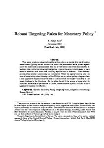
where yt is the level of output; y* denotes potential output; and xt again denotes a set of other variables.(3) Under this formulation, the path of short-term interest rates depends on realised values of the inflation and output gaps, with weights χ and δ respectively.(4) The model used in the policy simulations is a small, rational expectations macroeconomic model. The model is described in detail in the Appendix, but some of its main features are outlined briefly here. First, the model is open-economy. In the model, the exchange rate serves as an important transmission mechanism for monetary policy, through its effect on net exports and hence output, and through its effect on import prices and hence price inflation. Second, the model has several forward-looking features. The most important forward-looking variable is the exchange rate, which depends on the expected future path of short-term interest rates, domestically relative to overseas. As these interest rate expectations adjust, the exchange rate ‘jumps’ in response—as is observed among asset prices in the real world. In the model, all forecasts are formed rationally, in the sense that they are based on all useful information (including knowledge of the model and of the policy rule) and, on average, do not differ systematically from the eventual outcome. Third, consumer price inflation is also affected by expectations. This derives from forward-looking behaviour on the part of wage-bargainers when setting wages, as wages are a key component of consumer prices. Fourth, consumer price inflation also embodies a substantial degree of inertia or ‘stickiness’. This is an important feature of the model. It ensures that the time-series behaviour of inflation mimics that in the real world—which is slow-moving and persistent. Price stickiness ensures that nominal monetary shocks have persistent effects on real magnitudes, such as output and employment. This is again in line with the real-world behaviour of the macroeconomy. Finally, inflation inertia also ensures that there are transmission lags between implementing a change in monetary policy and its impact on output and inflation. These monetary transmission lags are a well recognised macroeconomic phenomenon. The model is calibrated in such a way that it matches the lagged and persistent response pattern of output and inflation following a monetary policy disturbance. Chart 1 illustrates the path of inflation and output resulting from a tightening of monetary policy, which aims to reduce inflation by 1 percentage point.

(1) There may be further, theoretical advantages to operating monetary policy according to an inflation forecast. For example, in some models, targeting an inflation forecast is equivalent to the fully-optimal rule (see Svensson (1996, 1997)). It may also help to improve monetary policy credibility by focusing inflation expectations. (2) Such as lags of short-term interest rates and the expected inflation rate in the next period. The latter term allows us to think of equation (1) as defining a path for short-term real interest rates. Batini and Haldane (op cit) discusses these features. (3) Which again includes lags of interest rates and the inflation rate expected next period. (4) In the original Taylor rule, these weights are both equal to 0.5.

61

Bank of England Quarterly Bulletin: February 1999

Inflation eventually ends up 1 percentage point lower. But the transmission mechanism is fairly slow and protracted. It takes up to two to three years for the new inflation equilibrium to be reached, one side-effect of which is a persisting contraction in output.

(the output gap) on the horizontal axis.(2) So points moving to the south-west in Chart 2 signal an improvement in policy performance—lower output and inflation variability—and conversely, points to the north-east signal a worsening policy performance.

Chart 1 Inflation and output response

Chart 2 Output-inflation volatility frontier

Percentage point changes from base

0.20

Output variability (σ, per cent)

+

1.8

0.00

– Output response

1.6

A (j = 0)

0.20 1.4 0.40 (j = 1) 1.2

0.60 Inflation response

B (j = 12)

0.80

1.0

(j = 4)

1.00

0.8

1.20 0

4

8

12 Quarters

16

20

0.6 0.0

24 0.7

Turning finally to the shocks, these are calibrated using the Bank of England’s core forecasting model (August 1997 version).(1) The exception is the exchange rate, where the shocks are the residuals from an uncovered interest parity condition, in turn derived using survey-based measures of exchange rate expectations.

Lags Lags in the transmission mechanism complicate the inflation control problem for monetary policy-makers. If policy-makers respond to deviations of current inflation from target, they will very probably be acting too late to offset effectively any build-up of inflationary pressures, because of these lags. Instead, they need to form and respond to expectations of future inflationary pressures, thereby allowing time for monetary policy to take its full effect. This then allows inflationary pressures to be headed off pre-emptively. Forecast-based policy rules, such as those in equation (1), have such a forward-looking dimension. In particular, they allow the policy-maker to align explicitly the horizon of the inflation forecast and the control lag for monetary policy. This is likely to improve inflation control, because the variable to which monetary policy is responding will also be the variable over which the authorities can exercise some degree of control. This point can be illustrated using simulations from the macroeconomic model and the policy rule outlined above. Chart 2 shows the results of one particular set of simulations. The variability of inflation is plotted on the vertical axis, and the variability of output relative to trend

0.9

1.1

1.3

1.5

1.9

2.1

2.3

2.5

Inflation variability (σ, per cent)

Each point in the chart gives the inflation/output variability pair associated with a simulation of the model under one particular specification of the policy rule. The line AB joins these simulation points. Moving along the locus of points from A to B, the simulations use a policy rule with a progressively more distant inflation forecast horizon. So for example, point A shows the pair of inflation/output variability points associated with the policy rule in equation (1) when j = 0—that is, when the policy-maker responds only to the current-period inflation rate. The next point along, moving from A to B, is the pair of inflation/output variabilities associated with a policy rule that responds to expected inflation one period ahead (j = 1). Because periods in the model are quarters, this is equivalent to responding to the inflation rate expected in the next quarter. For j = 4, policy is responding to the inflation rate expected one year (four quarters) ahead, and so on. Point B gives the pair of inflation/output variabilities associated with a policy rule that responds to expected inflation three years ahead (j = 12 quarters). Moving from point A to B, it is clear that lengthening the inflation forecast horizon initially helps to achieve a greater degree of both inflation and output-control; the locus moves to the south-west. The improvement in inflation control is marked, with inflation variability falling by almost 50%, comparing targeting current-period inflation with targeting an inflation forecast six quarters ahead. This is because of transmission lags, which mean that by responding to actual inflation, monetary policy is acting too late. Inflation control is disturbed. By having policy respond to what it is best able to control—

(1) The calibrated model outlined above does not have enough dynamic structure to ensure that its empirically estimated residuals are legitimate measures of original shocks. Using atheoretic time-series or VAR models to construct structural shocks is problematic because of the need to impose identification restrictions to unravel the structural shocks from the reduced-form VAR residuals. That is why shocks from the Bank’s core forecasting model were used. The Appendix discusses this in more detail. (2) Technically, variability is measured here by the square root of the average unconditional variance of each variable across 100 stochastic simulations.

62

1.7

Monetary policy rules and inflation forecasts

future inflation—inflation control can be improved dramatically.

turn minimises the extent to which output needs to be destabilised following an inflation shock.

Too distant an inflation forecast horizon can also lead to a worsening of policy performance, however, as Chart 2 illustrates. At inflation forecast horizons much beyond six quarters, inflation variability begins to increase. Monetary policy is, in these situations, doing too little to smooth inflationary shocks. Just as too near a forecast horizon can damage inflation control, so can too distant a horizon. In the model, the optimal forecast horizon lies somewhere in between, at around four to six quarters. This is where monetary policy has its largest impact on inflation; it is the horizon at which the authorities’ inflation control is, at the margin, greatest.

It is interesting to ask whether inflation forecast based rules could be improved by responding explicitly to output, rather than implicitly through the inflation forecast. Simulations from the model suggest that the gains in output stability from doing this are very small. Policy rules that respond only to inflation forecasts appear capable of synthetically recreating a similar degree of output stability to rules with explicit output terms in them. Certainly, the absence of output terms from an inflation forecast based rule does not in any way suggest a greater degree of output variability or a greater disregard for output objectives on the part of the policy-maker.

Because it is transmission lags that justify basing policy on inflation forecasts, the optimal forecast horizon will clearly depend on the length of these lags. The longer the monetary transmission lag, the further into the future is the optimal forecast horizon. Behavioural shocks that lead to a shortening of the transmission lag, such as a reduction in inflation inertia, ought also to be accompanied by a shortening of the policy horizon if inflation control is not to be upset.

Information

Output Monetary policy-makers in practice typically take account of output as well as inflation fluctuations in setting monetary policy. For example, the Bank of England Act 1998 states that the Bank’s objectives shall be: ‘(a) to maintain price stability; and (b) subject to that, to support the economic policies of the government, including its objectives for growth and employment’. Similar provisions can be found in the statutes of the European Central Bank in the euro area, and of the Federal Reserve Board in the United States under the Humphrey-Hawkins Act. On the face of it, an inflation forecast based policy rule, such as equation (1), appears to take no explicit account of output objectives; it responds only to expectations of future inflation. As Chart 2 illustrates, however, this impression is misleading. By altering the horizon of the inflation forecast, policy rules such as equation (1) can influence the variability of output in the economy. For example, according to Chart 2, lengthening the forecast horizon from zero (current-period inflation targeting) to four periods (one year ahead inflation-forecast targeting) causes output variability to roughly halve. The reason for this is that, at these more distant horizons, monetary policy has a more pronounced impact on inflation; the transmission lags have worked their way through. Because of its greater impact, monetary policy has to adjust less to offset a given inflationary shock. Touches on the brake and accelerator can afford to be lighter. This smaller adjustment in policy in

It is well known from optimal control theory that the optimal policy rule responds to all variables that offer useful information on the target variables of policy. To behave otherwise would be to restrict arbitrarily the information set of the policy-maker. Because they respond to only a subset of the available information, simple policy rules, such as the Taylor rule, are very likely to be inefficient by comparison with the fully optimal rule. Forecast-based rules are also likely to be inefficient for the same reason—they are simple and hence restrictive in their use of available information.(1) But there are good reasons for believing that forecast-based policy rules, although simple, may not be as restrictive and inefficient as other types of simple rule, such as the Taylor rule. An inflation forecast is formed using all information that is useful for predicting future inflation. That is, for example, how the forecasts published in the Bank of England’s Inflation Report are constructed. This means that even an apparently simple, forecast-based rule is implicitly responding to a wide and complex array of macroeconomic variables. The inflation forecast is simply serving as a summary statistic for this information. It is for this reason that forecast-based rules, though not as efficient in general as the fully optimal rule, may tend to be more efficient than other types of simple, backward-looking rule. Table A illustrates these points quantitatively. The set of rules is listed in the first column. They include the fully optimal rule; a variety of forecast-based policy rules, as in equation (1), for a range of values of the forecast horizon j, setting the feedback parameter α = 0.5; and a variety of Taylor-type rules, as in equation (2), for a range of values of χ and δ.(2) The second, third and fourth columns give the variability (standard deviation) of inflation, output and short-term interest rates associated with each of these rules. The final column gives an aggregate measure of the policy-makers’ welfare, by weighting together (somewhat arbitrarily) the variabilities in the second, third and fourth columns.(3)

(1) Except when using a specific kind of inflation forecast targeting rules, discussed in Svensson (op cit). (2) Omitting lags of short-term interest rates. (3) Output and inflation variabilities are equally weighted, while short-term interest rate variability is given a weight of one fifth this amount. The qualitative conclusions are not particularly sensitive to this choice of weights.

63

Bank of England Quarterly Bulletin: February 1999

Comparing optimal, inflation forecast based and Taylor rules Standard deviation of: output inflation

Welfare loss interest rate

Optimal rule 0.78

1.10

1.03

41.83

Inflation forecast based rules {j = 0} {j = 3} {j = 6} {j = 9}

1.52 1.07 0.91 0.94

1.19 1.17 1.34 1.57

0.92 0.61 0.51 0.40

76.37 52.61 54.18 68.04

Taylor-type rules {χ = 0.5, δ = 0.5} {χ = 0.5, δ = 1}

1.05 0.92

1.38 1.46

0.55 0.72

61.96 61.97

By definition, the lowest welfare loss comes from the fully optimal rule. It delivers both lower output and inflation variability than virtually all of the other rules. It is also, however, by far the most complicated of the rules considered in the table, responding to all variables in the model. As a result, the fully optimal rule would probably be impractical. It would be very difficult for the general public to monitor or understand effectively. All of the simple forecast-based rules perform somewhat worse than the optimal rule. Welfare losses are around 30% higher, even though certain rules are capable of matching the performance of the optimal rule on specific criteria—for example, in reducing inflation variability. However, these simple forecast-based rules perform favourably compared with simple Taylor rules. For example, the best-performing

64

Taylor rule delivers a welfare loss around 50% greater than the fully optimal rule. This is evidence of the greater information-efficiency of simple forecast-based policy rules compared with simple backward-looking rules. By responding, albeit implicitly, to a wider range of information variables, a forecast-based rule is able to deliver a greater degree of both output and inflation stability.

Conclusion Hypothetical interest rate rules for monetary policy have attracted considerable recent interest. But most such rules have tended to be based on current values of macroeconomic variables, such as output and inflation. So these hypothetical rules contrast somewhat with monetary policy behaviour in the real world, which tends to have a more forward-looking, forecast-based dimension. Policy rules that respond to forecasts of future inflation seem to perform well in quantitative simulations. These rules encompass, and can hence better control for the effects of, monetary transmission lags. They can ensure a suitable degree of output-smoothing. And they ensure that policy is responsive to most available information. These features allow better inflation and output control. The performance of hypothetical forecast-based policy rules offers support for the policy practice of basing monetary policy on forecasts of inflation and output, as is currently the case in the United Kingdom.

Monetary policy rules and inflation forecasts

Appendix

To assess the performance of rules (1) and (2) above, we used a small, dynamic open-economy linear rational expectations model. This Appendix offers a brief description of the model’s structure, properties, and calibration.(1) The model The model comprises four behavioural equations. Removing the constants in each equation and normalising to zero potential output and foreign variables, so that all variables represent deviations from equilibrium, the model can be expressed as: yt = δ 1yt-1 + δ 2[it-1 - Et-1πt] + δ 3qt-1 + eISt-1

(1A)

mt - pt = β1 yt + β2it + eLMt

(2A)

πt = ϕ 0 Et πt+1 + (1 - ϕ 0) πt-1 + ϕ1[yt + yt-1] + µ[(1 - ϕ 0) ∆qt - ϕ 0 Et ∆qt+1] + eπ t

(3A)

Et ∆qt+1 + Et πt+1 = it + eUIPt

(4A)

where yt is output, mt is nominal money, qt is the real exchange rate, πt is inflation, it is the nominal interest rate, and where ∆ is the first-difference operator (thus in equation (3A), ∆qt = qt - qt-1). Note that in equations (3A) and (4A), Et πt+1 denotes expected inflation where Et is the rational expectations operator. eISt-1, eLMt , eπ t , and eUIPt are disturbance terms or ‘shocks’, whose properties are described below. Equation (1A) is the IS equation. Output (yt) responds to the previous period’s values of the real interest rate and the real exchange rate. The real interest rate has a negative direct effect on output (δ 2 < 0) as higher rates depress expenditure, and an appreciation of the real exchange rate (ie a decrease in qt) produces a decline in output (δ 3 > 0), by reducing net exports. Equation (1A) indicates that output also depends on its lagged value (with coefficient 1 > δ1 ≥ 0). So output is predetermined, and monetary policy cannot affect current output. eISt is a vector of demand shocks. Equation (2A) is the model’s LM curve. Its arguments are conventional: a nominal interest rate, capturing portfolio balance (β2 < 0); and real output, capturing transactions demand (β1 > 0). eLMt is a vector of velocity shocks.

Equation (3A) is a supply curve. It is the open-economy analogue of Fuhrer and Moore’s (1995) Phillips curve specification (see Blake and Westaway (1996)).(2) The inflation terms—a weighted backward and forward-looking average—are the same as in the closed-economy case. There is some degree of inflation persistence (with weight ϕ 0), and some degree of forward-looking behaviour (weight 1-ϕ 0). The weights sum to unity, so that the Phillips curve is vertical in the long run. Prices also depend on the output gap, reflecting demand pressures. The inflation specification contains, in addition, (real) exchange rate terms, reflecting the price effects of exchange rate changes on imported goods in the consumption basket. Consequently, the monetary transmission mechanism that links the interest rate to inflation works through two channels in the model. There is a direct price channel— operating via the cost of imports, and an indirect real interest rate channel—affecting inflation via the output gap. Equation (4A) is an uncovered interest parity condition.(3) We do not include any explicit foreign exchange risk premium. The shock vector eUIPt comprises foreign interest rate shocks and other noise in the foreign exchange market, including shocks to the exchange risk premium. Model (1A)–(4A) is forward-looking in two ways. First, the uncovered interest parity condition is forward-looking, capturing conventional forward-looking behaviour in asset markets. In addition, the inflation equation is also forward-looking, reflecting forward-looking wage-bargaining behaviour. The parameters δ1 and ϕ 0 jointly govern the overall degree of forward-looking behaviour in the model. Calibration The model is calibrated on UK data. For the calibration, we set δ 2 = -0.5 (the real interest rate elasticity), and (δ 3 = 0.2) (the real exchange rate elasticity), in line with previous empirical estimates of IS curves. For the money demand equation, we set β1 = 1 and β2 = -0.5, so that money is unit income-elastic and has an interest semi-elasticity of minus a half, in line with empirical findings based on UK data in Thomas (1996). On the supply side, ϕ 0 is set equal to 0.2, which makes inflation predominantly backward-looking. This assumption appears to be more plausible empirically than an equally weighted backward and forward-looking inflation formulation (ϕ 0 = 0.5), both in the United States

(1) See Batini and Haldane (1999) (op cit) for a more detailed description. (2) This specification can be derived as the reduced form of a three-equation wage-price system. See Blake and Westaway (1996), Batini and Haldane (1999) op cit. (3) With the foreign interest rate normalised to zero.

65

Bank of England Quarterly Bulletin: February 1999

(Fuhrer (1997)) and the United Kingdom (Blake and Westaway (1996)). Finally, ϕ 1 (the output sensitivity of real wages) is set at 0.2, in line with previous studies.

Shocks A necessary step in generating impulse response functions is specification of the structural relationship between the various shocks. We assume that the innovations to these shocks behave in a recursive manner, in the order (eISt-1 → eUIPt → eπ t).(1)

(1) Money demand shocks are unimportant because they are fully accommodated under an interest rate rule.

66

Simulation of the model requires values for the standard deviation of the equations’ disturbances. We set the standard deviation of the IS, aggregate supply and money demand innovations, eISt-1 and eπ t, and eLMt equal to the estimated residual standard deviation from the output, earnings and money demand equations from the Bank of England’s core forecasting model (for the sample period 1989 Q1–97 Q3). The standard deviation of the uncovered interest parity shocks is estimated by generating a {eUIPt} sequence from equation (4A), using survey data on exchange rate expectations.

Monetary policy rules and inflation forecasts

References

Batini, N and Haldane, A G (1999), ‘Forward-looking rules for monetary policy’, Bank of England Working Paper No 91. Blake, A P and Westaway, P F (1996), ‘Credibility and the Effectiveness of Inflation Targeting Regimes’, The Manchester School, Vol LXIV, pages 28–50. Clarida, R, Gali, J and Gertler, M (1998), ‘Monetary Policy Rules in Practice: Some International Evidence’, European Economic Review, 42, pages 1,033–67. Fuhrer, J C (1997), ‘The (Un)Importance of Forward-Looking Behaviour in Price Specifications’, Journal of Money, Credit and Banking, Vol 29, No 3, pages 338–50. Fuhrer, J C and Moore, G R (1995), ‘Forward-Looking Behaviour and the Stability of a Conventional Monetary Policy Rule’, Journal of Money, Credit and Banking, Vol 27, pages 1,060–70. Stuart, A (1996), ‘Simple monetary policy rules’, Bank of England Quarterly Bulletin, August 1996, pages 281–87. Svensson, L E O (1996), ‘Price Level Targeting Versus Inflation Targeting; A Free Lunch?’, NBER Working Paper No 5719. Svensson, L E O (1997), ‘Inflation-Forecast-Targeting: Implementing and Monitoring Inflation Targets’, European Economic Review, Vol 41, pages 1,111–46. Taylor, J B (1993), ‘Discretion Versus Policy Rules in Practice’, Carnegie-Rochester Conference Series on Public Policy, Vol 39, pages 195–214. Thomas, R S (1996), ‘Understanding broad money’, Bank of England Quarterly Bulletin, May 1996, pages 163–79.

67