Does Pollution Increase School Absences?

Janet Currie Columbia University* Eric A. Hanushek Stanford University, E. Megan Kahn Amherst College, Matthew Neidell Columbia University, Steven G. Rivkin Amherst College

February 2008

* Currie is the corresponding author: Dept. of Economics, Columbia University, 420 118th St., New York, NY, 10025, [email protected]. We thank Alfonso Flores-Lagunes, Matthew Kahn, Walter Nicholson and Jessica Reyes and an anonymous referee for helpful comments as well as participants at the 2005 AEA meetings and the 2006 SOLE meetings.

Abstract We examine the effect of air pollution on school absences using unique administrative data for elementary and middle school children in the 39 largest school districts in Texas. These data are merged with information from monitors maintained by the Environmental Protection Agency. To address potentially confounding factors, we adopt a difference-in-difference-in-differences strategy that controls for persistent characteristics of schools, years, and attendance periods in order to focus on variations in pollution within school-year-attendance period cells. We find that high levels of carbon monoxide (CO) significantly increase absences, even when they are below the federal air quality standard. Our work suggests that the substantial improvements in CO levels in the air over the past two decades have yielded economically significant benefits.

Janet Currie Dept. of Economics, Columbia University 420 W 118th St., New York, NY, 10027 [email protected]

Matthew Neidell Columbia Mailman School of Public Health 600 W. 168th Street, 6th floor, New York NY 10032 [email protected]

Eric A. Hanushek Hoover Institution, Stanford University Stanford, CA 94305-6010 [email protected]

Steven G. Rivkin Department of Economics, P.O. Box 5000 Amherst, MA 01002-5000 [email protected]

E. Megan Kahn Dept. of Economics, Amherst College Department of Economics P.O. Box 5000 Amherst, MA 01002-5000

1

I. Introduction Even though substantial policy initiatives are aimed at reducing air pollution, uncertainty remains about the nature and extent of benefits from these actions. Existing epidemiological studies point to a variety of health impacts, but it remains difficult to assess the economic or social values of these impacts. It is also difficult to be confident that existing studies separate the causal impacts of pollution from correlated effects of neighborhoods, poverty, and a variety of household choices. We focus on how pollution affects school absences. By matching detailed schooling records with variations in the level of specific pollutants, we are able to establish a strong link to school absences. A large literature links child health and human capital attainment. Grossman and Kaestner (1997) summarize this literature and point to school absences as a major causal link in this relationship—children who miss a lot of school achieve poorer grades, are less engaged with school, and are more likely to drop out. Absences are also of concern to parents who have to miss work and to school districts because state funding frequently depends on attendance. In states where funding depends on student attendance, schools can lose as much as $50 per day per unexcused absence. Nonetheless, policy interventions that might reduce absences are less clear. Air pollution is a possible cause of school absence for some children. Children with respiratory problems such as asthma could be absent either because the pollution provokes an attack, or because parents keep the child at home in order to avoid pollution exposure. While absences are of interest in their own right, epidemiologists focus on absences as a possibly more sensitive proxy for health status than alternative measures such as emergency room visits or hospital admissions. Children are particularly sensitive to pollution given their small size, high

2

metabolic rates, and developing systems, making it important to have measures of the effects of pollution that capture its impact on the ability of children to perform their daily activities. This paper estimates the causal effect of air pollution on elementary and middle school absences using unique administrative data on schooling attendance in 39 of the largest school districts in the state of Texas. These data are merged with information about air quality from monitors maintained by the Environmental Protection Agency (EPA). It is difficult to identify a causal relationship between pollution and school attendance because of the influences of a number of potentially confounding factors. Absenteeism is affected by parental commitment to schooling, the opportunity cost of a child remaining at home, school policies, and of course health. Given extensive residential sorting -- based not only on wealth but also on preferences for school quality, environmental quality, peer characteristics, neighborhood amenities, and more -- geographic differences in pollution levels are correlated with family characteristics that may in turn be related to absenteeism. For example, pollution tends to be higher where people are poorer, and poor children may be more likely to be absent. In addition, seasonal differences in the prevalence of colds and flu as well as in pollution levels raise doubts about the use of seasonal variation in pollution levels to identify effects on absenteeism. In order to overcome these problems and try to identify causal effects, we adopt a difference-in-difference-in differences (DDD) strategy, in which we hold characteristics of schools, years, attendance periods and interactions of these variables constant, and focus on variations in pollution within school-year-attendance period cells.1 Hence, our models control not only for all stable characteristics of schools, years, and attendance periods but also for characteristics of school specific variations in particular years (such as unusual variations in the 1

In Texas, the school year is divided into six week intervals called attendance periods.

3

student body); for school specific patterns in particular attendance periods (such as higher rates of illness in winter); and for systematic variations in particular years and attendance periods (such as unusual weather patterns affecting multiple school districts). In addition, we also control for precipitation and temperature, two factors that affect air pollution levels and may also affect student health directly. Our evidence suggests that pollution affects school attendance. High levels of carbon monoxide (CO), including levels below the regulatory threshold set by the Environmental Protection Agency, increase absenteeism. This result is robust to alternative specifications, including models that permit the effects of pollution to vary by attendance period and grade level and models that include both leads and lags in pollution. Our results suggest that reductions in the number of days with high CO levels between 1986 and 2001 in areas with particularly high CO levels, such as El Paso, reduced absences by 0.8 percentage points, indicating a significant effect on school attendance. The rest of the paper is laid out as follows. Section 2 gives some background information about the health effects of pollution. Section 3 describes our data. Section 4 describes the methodology. Section 5 presents results, and section 6 summarizes the analysis and discusses implications for policy.

II. Background A. Pollution and Health Attention to air quality by the EPA is focused on six primary, or “criteria,” air pollutants: ozone, carbon monoxide, nitrogen dioxide, sulfur dioxide, particulate matter and lead. We focus on three of the pollutants (ozone, CO, and PM) that are most commonly tracked by air quality

4

monitors. We dropped separate consideration of nitrogen dioxide because there is no federal standard for these emissions, but nitrogen dioxide is one of several nitrogen oxides that are key components of ozone formation, which we do examine. Data on lead were not available for this study, and airborne lead levels during the 1990s tended to be quite low.2 Although data on sulfur dioxide (SO2) were available, SO2 levels are low enough now that it is not a primary concern. In addition, many of the SO2 monitors have been removed over time. Although pollution levels in the U.S. are dropping, high levels remain in many localities. The EPA estimates that 160 million tons of pollution are emitted into the air each year in the U.S. and that 146 million people were exposed to air that was considered unhealthy at times in 2002 (EPA, 2003). Many more people are routinely exposed to levels that fall below EPA thresholds but might still cause adverse health effects, as there remains uncertainty over the appropriate threshold levels.3 Relatively little is known about the exact mechanisms underlying any health effects, although most pollutants affect the respiratory and cardiovascular systems. Even less is known about the effects of pollutants on children, although it is thought that children are more susceptible to the effects of pollution than adults because their bodies are still developing and because they have higher metabolic rates. For example, a child exposed to the same air pollution source as an adult would breathe in proportionately more air, and suffer proportionately greater

2

See Reyes (2003) for a study of the effects of removing lead from gasoline.

3

The 24 hour Air Quality Standard (AQS) for PM10 is 150 µg/m3. The 8 hour AQS for ozone is .08 parts per

million (80 ppb). The AQS for CO is 9 ppm. For more information about these standards see: http://www.epa.gov/air/criteria.html.

5

exposure. Children also typically spend more time outdoors than adults, increasing their total exposure. Most studies exploring correlations between air pollution and health focus on particulate matter, which is a catch-all term for pollution particles that come from many different sources and can be of different sizes and compositions. Because only small particles can be inhaled into the lungs, the standard is to look at particulate matter less than 10 micrograms per cubic meter of air, or µg/m3, in aerodynamic diameter (PM10), and that will be our focus here.4 PM10 has been shown to aggravate and increase susceptibility to respiratory and cardiovascular problems, including asthma. Children and people with existing health conditions are most affected. The leading theory about why PM10 affects health is that it provokes an immune system response. If, however, immune responses take time to develop, it may be difficult to detect any effect of short-term movements in PM10 on health outcomes (Dockery, 1993, Hansen and Selte, 1999, EPA 2004, Samet, 2000, and Seaton, et al. 1995). Ozone (O3) is a secondary air pollutant formed by nitrogen oxides and volatile organic compounds in the presence of heat and sunlight. These compounds come from exhaust, combustion, chemical solvents and natural sources. Ozone has been associated with many respiratory problems and is known to seriously aggravate asthma. Levels rise with the temperature, peaking on hot summer afternoons. There is a considerable amount of within-day variation in ozone levels as the temperature and sunlight changes, with higher levels occurring 4

Fine-particulate air pollution, which includes particles less than 2.5 µg/m3 (PM2.5), is considered by many experts

to be a more appropriate measure of harmful pollutants because smaller particles are more likely to be made up of toxic materials (such as sulfate and nitrate particles left over from fossil fuel combustion). However, most regulatory agencies only began collecting information on PM2.5 in the past few years, so data on PM2.5 was not available during the period examined in this paper.

6

during the hours people are most likely to be outside. Children who play outside are especially susceptible to ozone. Ozone poses less of a threat indoors, since it quickly reacts with surfaces and becomes harmless. After rising for some time, ozone levels have dropped dramatically in recent years, falling back to their 1980 level in 2003 (EPA 2003, and Lippmann, 1992). Carbon monoxide is emitted from incomplete combustions occurring in fires, internal combustion engines, appliances, and tobacco smoke. Cars account for as much as 90 percent of CO in some urban areas. By bonding with hemoglobin in the blood, CO impairs the transport of oxygen in the body, leading to cardiovascular and respiratory problems. People with preexisting cardiovascular or respiratory problems appear to be most susceptible to exposure. Levels are highest during cold weather (Lippmann, 1992 and EPA 2004). The large clinical literature regarding the health effects of pollution has focused primarily on showing associations between air pollution and adverse health outcomes among adults. Nonetheless, because the health of adults reflects a lifetime of exposures in various locations, exposure in their current area of residence may not be a good measure of the effects of pollution. A smaller literature examines health effects among infants and children, who are more likely to have lived in their current location since birth. This literature has shown associations between air pollution and infant mortality, as well as hospitalizations for respiratory conditions. However, causal interpretations of these estimates may still be confounded by the fact that pollution tends to be higher in poor and minority areas. Hence, one might expect people in high pollution areas to have worse health for other reasons. In two important and innovative works, Chay and Greenstone (2003a, b) used changes in regulation to identify pollution’s effects on infant mortality. They argue that the 1970 and 1977 Clean Air Acts caused exogenous changes in pollution levels and that the changes varied across

7

areas. These changes can be used to examine pollution’s effects on housing markets and infant mortality. They find that a 1µg/m3 reduction in total suspended particulates (a common measure of overall pollution at that time) resulted in 5-8 fewer infant deaths per 100,000 live births. Currie and Neidell (2005) examine the effects of air pollution on infant deaths in more recent data. They use individual-level data and within-zip code variation in pollution over time to identify the effects of pollution. They include zip code fixed effects to account for omitted characteristics like ground water pollution and socioeconomic status, and find that reductions in two pollutants – CO and PM10 – in the 1990s saved over 1,000 infant lives in California. Pollution has also been shown to have effects on morbidity as well as mortality. In a recent study, Neidell (2004) uses within-zip code variation in pollution levels to show that air pollution affects child hospitalizations for asthma. In particular, he finds that if CO levels had been at their 1992 levels in 1998, hospital admissions for asthma would have been 5 to 14 percent greater among children 1 to 18. This is one of the only preceding studies to establish a causal relationship between current levels of pollution and child health.5 B. Pollution and Absenteeism As discussed above, absences can be viewed as a proxy for child health that is more sensitive to pollution induced diseases than hospital related measures. There may be a great deal of illness that is not severe enough to send a child to a hospital, and absence data offers a window on these illnesses. Moreover, there is a long tradition of using absence from school to define disability among children. Of course pollution is not the only reason for school absences, making it imperative to account for other causes that might confound the estimates. Most absences are due to illness and 5

The “Moving to Opportunity” experiment in which some residents of public housing projects were randomly selected to be eligible to move to low poverty neighborhoods were associated with reductions in asthma, although this is not necessarily due to differences in exposures to air pollution (see Katz, Kling, and Liebman, 2001).

8

are attributable either to respiratory infections or to gastroenteritis (Gilliland et al., 2001). However, given the many other factors that can cause absences, it is clearly important to control adequately for a wide range of variables. For example, low socioeconomic status might be correlated both with high exposure to pollution and with high absence rates. Cold, wet weather will contribute to both higher illness and lower pollution levels. A key difference between economic models and epidemiological models of the effects of pollution is that economists anticipate that parents can respond to potential air pollution through locational choices. Parents can avoid air pollution by moving to neighborhoods with cleaner air, making neighborhood choice an element to consider in modeling the impacts of pollution. Parents and schools can also respond to pollution by keeping children indoors when the air is particularly unhealthful. The decision to keep a child home from school directly adds to absences, and school decisions to keep children indoors may indirectly increase absenteeism if recess indoors contributes to the spread of colds and flu. We cannot distinguish between absences caused by the direct health effects of pollution and absences caused by avoidance behavior. Nonetheless, to the extent that children miss school in order to avoid pollution, they and their parents still incur a cost, and it is useful to capture this type of avoidance behavior as well as the direct effect of pollution on illness in assessing the total costs of pollution. The recent literature examining the link between absenteeism and pollution is summarized in Chart 1.6 Most studies focus on associations between pollution and absences

6

One of the first studies of this topic is by Ferris (1970). He studies approximately 700 students from seven

schools in Berlin, New Hampshire. He found no difference in the mean levels of absences between schools.

9

rather than on the identification of causal linkages and control for omitted variables in only a limited way. One of the most convincing studies is by Ransom and Pope (1992) who examine the impact of PM10 on absenteeism in the Utah Valley. Their data encompass a period from August 1986 to September 1987 when a steel mill, the major polluter in the valley, shut down and pollution levels fell dramatically. That is, much of the variation in pollution over their sample was due to an event that families had little control over and were unlikely to have responded to in the very short run. They find that absences were 54 to 77 percent higher when PM10 increased from 50 to over 100 ug/m3. These estimates imply that about one percent of students in their sample were absent each day as a result of particulate pollution exposure. In addition, they find that the effect of high PM10 levels on absenteeism persisted for 3 to 4 weeks. This persistent effect may complicate attempts to measure responses to short term fluctuations in this pollutant. One important concern with this analysis is the possibility that the job loss following the steel mill closure directly affect absences by reducing the cost of taking care of a child home from school or adversely affecting families and children in ways that reduced school attendance. A second notable study is by Gilliland et al. (2001) who use data from the Children’s Health Study to investigate the effects of pollution on absences due to a number of causes, including respiratory illness. The authors monitored a cohort of 2,081 4th grade children in 12 southern Californian communities from January through June 1996. They focus on the relationship between absence rates and within-community deviations in pollution, and allow for lagged effects of pollution. They find that a 20 parts per billion (ppb) increase in O3 was associated with a 63 percent increase in absences for illness, and an 83 percent increase in absences for respiratory illnesses. Absences reached a peak five days after exposure.

10

They also find that, while average PM10 levels were associated with higher absence rates, daily increases were associated only with non-illness-related absences. They find this result puzzling, but it could reflect insufficient controls for differences in family background or other variables that are correlated with higher pollution levels. Another possibility is that small cell sizes make the results sensitive to outliers. The other studies included in Chart 1 have weaker designs for identifying causal impacts. Chen et al. (2000), however, is notable because it is the only previous study to have examined CO. Although CO is known to be dangerous (exposure to high levels is fatal), it has been largely ignored in the epidemiological literature on the effects of pollution and health. Chen et al. (2000) find that an increase of 1 part per million in CO increased absence rates by almost 4 percent. Like Gilliland et al. (2001), they also find a curious negative correlation between PM10 levels and absences. Our study is the first to use panel data methods in a large sample in order to try to estimate the causal effect of air pollution on absenteeism. As we describe in detail below, identification in our models is based on school differences in the year-to-year variation in pollutant and absence levels within attendance periods. Because we control for seasonal patterns in attendance at each school, idiosyncratic factors affecting a particular school and year, and special factors affecting all schools in a particular year and attendance period, the remaining pollutant differences provide a plausibly exogenous source of variation with which to identify the causal effects of the respective pollutants.

III. Data

11

Our analysis centers on Texas, which as a large industrial state is a major producer of pollution. In 1998, Texas ranked first in the nation in emissions of nitrogen oxides and volatile organic compounds (the two components of ozone), and second in emissions of CO and PM10 (EPA 1998). According to the American Lung Association, the Houston and the Dallas-Fort Worth metropolitan statistical areas rank fifth and tenth, respectively, in listings of areas with the worst ozone pollution in the country. With high and variable levels of pollution, Texas provides a good environment in which to examine the effects of air pollution on school attendance. This paper uses panel data for schools within 10 miles of pollution monitors in 39 of the largest school districts in Texas –accounting for roughly 40 percent of the students in grades one through eight in the Texas public school system – for the academic years 1996 through 2001. There are 1,512 schools with pollution information in this sample. Two different sources of data are used, one for pollution and one for attendance. Using the latitude and longitude of each school and monitor, schools are matched with the closest pollution monitor. The absence data are only available in aggregated six week attendance period blocks, so the hourly pollution data are also aggregated into six week blocks based on school-specific dates for the attendance periods.7 The school data in this paper come from the Texas Schools Project of the University of Texas, Dallas. The database combines data from a number of different sources and contains student level information for all public school students and teachers in Texas, along with information about the schools themselves. In addition to information about absenteeism, we also use data on gender, family income and ethnicity.8 Because all students in a school are exposed 7

Since the school calendars vary from district to district, each district was contacted in order to establish beginning

and ending dates for each 6 week period in each year. 8

By using school absences we are necessarily limited to days when school is in session and therefore omit a large

share of the summer period. Although ozone is highly correlated with temperature, it typically peaks in Texas in

12

to the same pollutants, we aggregate the data by school, attendance period, and year to produce the school average absentee rates and demographic characteristics for each six week attendance period in each year. In preliminary work we examined the possibility that pollution effects differed by ethnicity or family income but found no evidence of significant differences. All regressions are weighted by the number of student observations in the cell. The final sample includes over 12 million student by attendance period observations. The pollution data come from the Texas Commission on Environmental Quality (TCEQ), formerly the Texas Natural Resource Conservation Commission (TRNCC). Individual monitors for each pollutant are set up all over the state and take hourly readings of the pollution levels at each location.9 In order to allow for non-linear effects of pollution we measure pollution relative to EPA thresholds and allocate each day into one of five categories separately for each pollutant: 0-25%, 25-50%, 50-75%, 75-100% and greater than 100% of the relevant threshold. We then calculate the shares of days in each category for all six-week attendance periods.10

late August and September when children have returned to school, so we still capture the time of year when ozone levels approach or exceed Air Quality Standards, as Table 1 indicates. 9

Over the years of this analysis, the numbers of monitors for each pollutant changed as some were taken on and off-

line. In our sample, the number of O3 monitors increased from 29 to 41 and the number CO monitors ranged between 20 and 24 between the 1996 and 2001 school years. The number of PM10 monitors actually fell from 38 to 26 between the 1996 and 1998 school years before rising to 31 in the 2001 school year. Changes in the sample composition over time due to changes in the number of monitors are one of the things that will be controlled by the inclusion of school-by-year fixed effects. 10

Attendance periods with fewer than 25 days of CO and ozone data and five days of PM10 data are excluded from

the sample. We set the PM10 threshold lower because PM10 readings are recorded roughly every sixth day in many locales rather than daily.

13

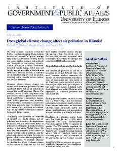
Figures 1 to 3 provides descriptive information about patterns of absences and pollution levels by attendance period for CO, ozone, and PM10. The statistics are calculated using data aggregated to the state, year, and attendance period level and are weighted by cell sizes for the 21,791 cells. Figures 1-3 report mean absence rates and the percent of days each pollutant exceeds 75% of the threshold by attendance period. Absences and pollution levels vary systematically across attendance periods. Absences reach their highest level in the fourth attendance period (winter) and are lowest in the first attendance period (early fall). CO generally follows this pattern, though the profile has changed over time. In 1995, the second attendance period had the highest pollution levels, while the highest in 2000 was in the fourth period. Ozone displays the reverse pattern, peaking at the beginning of the school year and dropping during the winter. PM10 peaks in the second attendance period (late fall), but are also relatively high in the fourth and fifth periods (late winter or early spring). Figures 1 and 2 also demonstrate that CO and PM10 levels fell considerably over the study period. The largest decline was in CO, which fell by a substantial 42%. O3 levels surprisingly increased from the previous year in three of the six years (not shown), and showed no overall trend. Figure 4 displays a comparable plot but focuses on Bowie High School in El Paso, one of the most polluted school districts.11 The figure illustrates that some areas had much higher pollution levels than the averages seen in Figure 1 to 3. For example, in the second attendance period in 1995, one out of every eight days at Bowie High School had CO over 75% of threshold. By 2000, the situation had improved substantially, as they had no days over the 75% threshold. This school is 0.16 miles from a CO/ozone monitor and 1.6 miles from a PM10 monitor, so that pollution is very accurately assigned. The highest CO cells in our data were 11

Due to confidentiality requirements, attendance data can not be displayed for an individual school.

14

located in El Paso, Laredo, and Houston, while the highest PM10 cells were located in Galveston and Hidalgo counties. The data indicate that O3 consistently moves in the same direction as temperature, so that differences in ozone pollution from year-to-year are primarily based on changes in average temperature. This highlights the importance of controlling for temperature in the analysis, since temperature might have independent effects on illness and absences. Precipitation is also likely to be important. On the one hand, it cleanses pollutants from the air. On the other hand, rainy weather may be associated with increased absence for illness regardless of the level of pollution. Table 1 shows the share of child-level observations in each absence or pollution category cell, by the child’s race and by whether or not the child was receiving a subsidized school lunch (the best available measure of a child’s socioeconomic status in the data).12 Blacks and Hispanics have somewhat more absences on average than non-Hispanic whites, and school lunch children have more absences than those who do not participate in the program. Turning to the pollution measures, Hispanic children are more likely to be exposed to high CO and PM10 days than either blacks or whites, but are less likely to be exposed to high ozone days. Similarly, school lunch children are more likely to be exposed to CO and PM10 and somewhat less likely to be exposed to high values of ozone. This table suggests that poor and minority children are generally more likely to be impacted by CO and PM10 exposure.

IV. Methods

12

Families with incomes less than 130 percent of the federal poverty line are eligible for free school lunches, while

families with incomes less than 185 percent of the poverty line are eligible for reduced price meals. This is the best measure of household economic status available in these administrative data.

15

A number of factors complicate efforts to identify the causal effect of pollutants on absenteeism. Both variables that determine pollution levels and those that determine the distribution of families among communities can directly affect absenteeism, making it necessary to account for a number of potentially confounding influences. For instance, if poor or minority families are more likely to live in heavily polluted areas and also have higher absence rates due to factors other than air pollution, such as less access to preventative medical care, then we may obtain spuriously large positive effects of pollution on absences. Given limited information on both family background and pollution determinants, it is unlikely that OLS regression models attempting to control for these other influences would produce valid causal estimates. To remove the influences of key confounding factors, we exploit the panel nature of our data to account for unobserved differences in schools, seasons, and years by estimating the following difference-in-difference-in differences (DDD) model: 4

(1)

absencespy = ∑ pollution spyi π i + X spy β X + weatherspy β W + grade spy β G + school s + i =1

period p + yeary + school * period sp + school * yearsy + year * period yp + ε spy where absence is the average percentage of days that students are absent in the school, year, and period; pollution is a vector of measures of the three pollutants; X is a vector of student demographic characteristics, including the shares of students who are Asian, Hispanic, and black (whites are the omitted category), the share of students eligible for a subsidized lunch, and the share of females in each school-by-attendance period-by-year cell; weather includes measures of temperature and precipitation; grade is a vector containing the shares of students in each grade omitting one; school is a vector of school fixed effects; year is a vector of year dummies; period is a vector of attendance period fixed effects; and period*year, school*period, and school*year are vectors of interactions between these variables. Because all students in a school receive

16

identical pollution treatments, and because attendance data is only available at the level of the attendance period, we aggregate over students, making the unit of observation a school, year, and attendance period cell. All regressions are weighted using cell sizes and standard errors are clustered at the monitor, attendance period, and year level to account for common shocks within the cluster. In order to allow for nonlinear pollution effects and to examine the link between federal threshold levels for pollution and absenteeism, we measure pollution using a series of dummy variables for the fraction of days in the attendance period in which pollution lay between 25-50 percent of the threshold, 50-75 percent of the threshold, 75-100 percent of the threshold, or was greater than 100 percent of the threshold, with 0 to 25 percent the omitted category. The aggregation of pollution within an attendance period precludes identification of the precise timing of pollutant effects since the pollutant coefficients provide the cumulative effects of a pollution event on absences regardless of time after exposure. The inclusion of X and the school fixed effects help to account for persistent differences in average student characteristics that might be correlated with absences. The grade shares account for any systematic differences in absenteeism related to age. Year dummies control for trends in attendance rates, and period dummies control for seasonal effects. The pair wise interactions between school, year, and period control for many other factors that might be related to absences. For example, school*year effects account for changes over time in student populations, the degree of attendance enforcement efforts, and annual local weather variation, while period*school effects help to account for distinctive seasonal patterns within schools (for example, schools with high immigrant enrollments might routinely experience high absences

17

surrounding the Christmas vacation period). Finally, year*period effects help to account for unusual seasonal effects common to all districts, such as an unusually bad flu season. Given this extensive set of controls, the causal effect of pollution is identified by variation at the year-school-period level. Consider first absences and pollution levels at a single school. The inclusion of school by year fixed effects accounts for year specific factors common to all attendance periods, while the inclusion of school by attendance period fixed effects accounts for attendance period specific factors common to all years. This can be viewed as a difference in differences model, where the “effect” of pollution is identified by differences across attendance periods in the year-to-year differences in pollution levels. One potential problem with this model is the possibility that statewide factors could introduce attendance period specific changes in absences over time that could contaminate the estimated pollution effects. Fortunately, the availability of data for a number of schools enables us to control for average period-by-year effects across all schools to account for unobserved differences by attendance period and year common to all schools that could bias the estimates. The inclusion of school-byyear, school-by-attendance period, and attendance period-by-year fixed effects and other variables that differ by school, attendance period, and year (the DDD Model (1)) thus controls for myriad potentially confounding factors. The DDD models generate consistent estimates of the effects of pollution as long no other factors systematically affect both pollution and absences at the school-year-period level. An example of something which would violate this identification assumption would be a natural disaster (such as a forest fire) which increased air pollution levels and also resulted in increased absences in a particular school, year, and period. We are not aware of incidents of this type within our sample period.

18

Understanding what drives the residual variation in pollution, and whether it is orthogonal to omitted variables that cause absences, is essential for understanding how our procedure identifies the effect of pollution. The vast majority of emissions are relatively stable over short time periods and are not driven by changes in local economic conditions. Therefore, the variation in ambient pollution levels is primarily driven both directly and indirectly by changes in environmental conditions, such as weather. For example, in colder weather, CO levels increase because the cold air slows its conversion to carbon dioxide. Additionally, people may idle their cars for longer periods of time or use more fuel to heat their homes, further increasing CO levels. While we control for weather, it is likely that the same weather pattern and the same individual responses will lead to substantially different pollution outcomes in different areas. In a rural area with few sources of emissions, the incremental pollution is unlikely to push measured pollution above any threshold. In a dense area, however, where considerably more emissions exist, the same changes could substantially worsen overall air quality. Similarly, differences in topography, such as mountains that trap pollutants, can interact with changes in weather to create different levels of air quality. A key feature of our identification strategy is the assumption that individuals in different areas react to changes in weather in a similar way regardless of the implications of their actions for overall air quality. Under this assumption, relevant changes in behavior are uncorrelated with idiosyncratic changes in air quality, and we can focus on how absences relate to these exogenous variations in pollution. V. Results a) Main results

19

Table 2 reports estimates of variants of equation (1) for all schools within 10 miles of a pollution monitor, with standard errors clustered at monitor, attendance period, and year level. The first column shows ordinary least squares (OLS) estimates of models similar to (1) except it excludes the interactions between period and year, school and period, and school and year. These estimates suggest that air pollution is positively associated with school absences. More specifically, CO levels between 75 and 100% of the Air Quality Standard (AQS), ozone levels over 100% of AQS, and PM10 levels between 75 and 100% are associated with a statistically significant increase in absences. Although we find some positive associations, a concern with these estimates is that we do not find a monotonically increasing relationship between the pollutants and absences. For example, the effect of CO is larger in the 75-100% category than in the over 100% category, suggesting the possibility of unobserved confounding. The second column of Table 2 shows our preferred DDD estimates. These estimates also indicate higher pollution levels associated with more absence (though only for CO) but provide evidence of a more consistent relationship. In these models, both CO levels between 75 and 100%, and those above 100% of AQS are associated with significantly higher absence rates. We do not, however, find a statistically significant association between absences and either ozone or PM10 in the upper pollution categories. For CO, we also find evidence of a monotonically increasing pattern consistent with a causal relationship between CO and absences: the coefficient in the over 100% category exceeds the coefficient in the 75-100% category, which exceeds that in the 50-75% category. Since we did not find this pattern in the OLS estimates, this strengthens the case for preferring our DDD estimates. In terms of magnitude, the estimates for CO imply that an additional day between 75 and 100% of the threshold increases absenteeism by 5 percentage points, while an additional day

20

with a CO level above the AQS increases absenteeism by almost 9 percentage points.13 Although such high levels of CO are not commonplace during this period, 66 school-byattendance period–by-year cells had levels above 75% at least 10% of the time. Thus the estimates imply increases in the average absenteeism rate in a period of roughly one half a percentage point in these cells. This is a significant effect but much smaller than that reported by Chen et al (2000) who did not control as thoroughly for potential confounders. The DDD estimates in column 2 also suggest a few anomalous findings for ozone and PM10. For example, we find ozone levels between 25 and 50% or 50 and 75% of the threshold have significant negative effects on absences relative to the omitted 0 to 25% of threshold category. Moreover, only PM10 level between 50 and 75% of the EPA threshold has a statistically significant effect on absences, while higher levels do not, suggesting a possible nonmonotonic relationship between PM10 and absences. While it is possible that these estimates may reflect omitted variable bias, the estimated coefficients in all of these anomalous cases are very small – an order of magnitude smaller than those discussed above for CO. Another possibility is that dividing each levels of each pollutant into five categories asks too much of the data. Hence, in columns (3) and (4) of Table 2 we estimate models with dichotomous cutoffs. Column (3) focuses on pollution levels over 75% of the threshold, while column (4) focuses on pollution levels over 100% of the threshold. The estimated effects of pollution levels above these cutoffs are very similar to those shown in column (2), providing further support that only high levels of CO affect school absences. 13

Technically, the estimates say that if the share of high pollution days in the attendance period increased to 100

percent, then absences over the attendance period would increase by either 9 or 5 percentage points. We can assume that this relationship also holds for daily attendance, as long as daily attendance is affected by daily pollution levels (rather than by cumulative pollution levels over several days, for example).

21

The fifth column of Table 2 shows additional estimates of equation (1) for models in which we add each pollutant separately. That is, while each of the previous columns shows estimates from a single equation, column (5) shows estimates from three separate models, one for each pollutant. The estimates are very similar to those in column (2) suggesting that multicollinearity is not impacting our analysis and that we obtain much the same results from single pollutant models. b) Robustness checks Since we primarily find an association between CO and school absences, we focus our specification checks only on CO. Table 3 shows that our results are robust to several changes in specification. In order to investigate the potential effects of measurement error in pollution, we assume that pollution is more accurately measured in schools that are closer to a monitor. Column (1) shows estimates based on a sample of schools within 5 miles of a monitor. Although imposing this restriction reduces the number of observations considerably, the estimates remain statistically significant for the two highest CO categories and are similar to those shown in Table 2. Since attendance periods 2 3, 4, and 5 had a relatively high number of days with CO above 75% of the threshold, columns (2) to (5) show separate estimates for these attendance periods from specifications estimated separately for each attendance period.14 Note that these are difference-in-difference models, not DDD models. The coefficients for CO levels between 75 and 100 percent of the threshold are all positive and fairly similar in magnitude to those shown in Table 2 (with the exception of attendance period 2 where the estimate is much smaller). The estimates for attendance periods 3 and 4 are significant at the 90% level of confidence.

14

Period 1 had no days above 75% of the threshold, while in period 6 only one school had one day above 75% of the EPA threshold.

22

The coefficients on the share of days above the threshold are positive and significant in period 2, and not statistically significant in any other periods. However, this is not surprising given the very small number of days above the threshold in the other attendance periods. Columns (6) and (7) show separate estimates for children in grades 1 to 3 and in grades 4 to 8. As discussed above, the previous literature suggests the effects of a given level of pollution may be greater for smaller children. We find that the effect of violating the standard is 1.5 times greater for younger children, while the estimated effect of CO levels between 75 and 100% of the standard is 1.3 times larger for older children. However, we cannot reject the null hypothesis of similar effects for both younger and older children, though we recognize that this crude test ignores many other differences between younger and older children that might affect these estimates. More importantly for our analysis, the consistent estimates of a positive effect of CO on absences provide further evidence of the robustness of our estimates. As a final robustness check, Table 4 shows estimates of models that include two leads and two lags of CO in addition to current values. Lead values of pollution should not impact current absences, so finding an effect of leads would suggest misspecification. Lagged values may have either a positive effect if the biological effects of CO are cumulative or long-term or a negative effect if parents respond to previous absences by reducing current absences. The first panel shows estimates from specifications similar to column (2) of Table 2. The estimated effects of current CO exposure are very similar to those discussed above. Among the lags, we find a statistically significant negative coefficient on CO levels between 75 and 100% of the threshold, consistent with the possibility that the behavioral channel dominates the biological one: high pollution levels last period that increased absences in that period led parents to reduce absences in the current period. We also find a statistically significant coefficient on

23

the second lag of CO levels between 25 and 50% of the threshold, but this coefficient is very small. Among the leads, there is only one coefficient (on the one period lead of CO between 75 and 100% of threshold) that is statistically significant and it is negative. The coefficient on the one period lead of CO above 100% is of a similar magnitude and positive, though it is not statistically significant. This pattern of sign switching suggests that including 10 leads and 10 lags may be too demanding on the data. In the second panel of Table 4, we show models with 3 pollution categories in which the top category is pollution over 75% of the threshold. In this specification, none of the leads are statistically significant. The lagged value of CO levels over 75% is significant and negative, which is consistent with the notion that parents whose children were absent in the last period try to avoid absences in the current period. The coefficient on the indicator for current CO levels over 75% of the threshold is also quite similar to that shown in Table 2. This pattern of results supports the evidence that high current CO levels have a causal effect on absences.

VI. Conclusion Obtaining convincing estimates of the causal impact of air pollution on health is difficult. Two major obstacles to this effort are the presence of confounding factors brought about through residential sorting and the lack of health measures that capture the range of morbidities purportedly related to pollution. By merging administrative school-level panel data with pollution monitor data, we hold fixed school, year, and attendance period characteristics constant in order to control for many potentially confounding factors. Furthermore, by linking air quality

24

directly with school absences, we focus on a sensitive measure of children’s health and morbidity. Our major finding is a significant and robust effect of CO on school absences, both when CO exceeds air quality standards (AQS) and when CO is 75-100% of AQS. Although the number of days where CO approaches these levels is quite low in most jurisdictions over the time period we study, this has not always been the case. For example in 1986 in El Paso, an area with particularly high CO levels, there were 16 days that CO exceeded AQS and 19 days where CO was between 75 and 100% of the threshold. The respective numbers in 2001, the last year for which we have attendance data available, are 1 and 6. Based on our econometric estimates, this decrease in high CO days decreased absences in the 2000-01 school year by 0.8 percentage points, a significant change compared to the baseline absence rate in all of Texas of 3.58%. Since improvements in air quality over time are largely due to air quality regulations (Henderson, 1996, Chay and Greenstone, 2003b), this suggests that air quality regulations are having a positive impact on children’s health. These effects become more pronounced if we consider that the effects of pollution on vulnerable segments of the population, such as asthmatics. Although we cannot identify asthmatic children in our data, we provide the following back-of-the-envelope calculation to assess the possible magnitude of effects for asthmatics in El Paso. The asthma prevalence rate in 2002 for school age children in the U.S. is 14.0 percent and, conditional on being absent, the probability the child has asthma is 28.3%.15 Based on the mean absence rate in our sample of 3.58%, this implies an absence rate of 7.2% among asthmatics. If all of the 0.8 percentage point

15

Based on authors’ calculations from the 2002 National Health Interview Survey.

25

reduction in absences in El Paso occurred among asthmatics, this would imply that the absence rate among asthmatics was reduced by roughly 44%. Our findings for CO, combined with those of previous studies documenting a robust effect of CO on different populations and health outcomes (Currie and Neidell, 2005, and Neidell, 2004), is relevant for the continuing debate over regulations concerning automobile emissions (Barnes and Eilperin, 2007). Automobiles are a major source of CO in urban areas, contributing as much as 90% of CO emissions. There are continuing discussions about the relative merits of the primary approaches for reducing CO emissions: technological innovations in fuel combustion (such as catalytic converters), development of alternative fuels that do not emit CO (such as ethanol, biodiesel, and fuel cells), and reductions in vehicle miles traveled. Our findings cannot address the efficacy of these alternatives, but they do point to significant additional channels for obtaining benefits from reductions in CO emissions.

26

References Action for Healthy Kids, 2004. “Students’ Poor Nutrition and Inactivity Comes With Heavy Academic and Financial Costs to Schools,” Sept. 2004. http://actionforhealthykids.org/filelib/pr/PoorNutritionIncursCosts-PressRelease.pdf Barnes, Robert and Juliet Eilperin. “High Court Faults EPA Inaction on Emissions,” Washington Post, April 3, 2007, A01. Bridges to Sustainability and Mickey Leland National Urban Air Toxics Research Center. 2003. “Final Report: Assessment of Information Needs for Air Pollution Health Effects Research in Houston, Texas.” Feb. 17, 2003. Chay, Kenneth and Michael Greenstone 2003a. “Air Quality, Infant Mortality, and the Clean Air Act of 1970.” NBER Working Paper #10053. Chay, Kenneth and Michael Greenstone 2003b. “The Impact of Air Pollution on Infant Mortality: Evidence from Geographic Variation in Pollution Shocks Induced by a Recession.” Quarterly Journal of Economics 118(3): 1121-1167. Chen, Lei et al. 2000. “Elementary School Absenteeism and Air Pollution.” Inhalation Toxicology. 12: 997-1016 Currie, Janet and Neidell, Matthew 2005. “Air Pollution and Infant Health: What if We Can Learn From California’s Recent Experience?” Quarterly Journal of Economics, 120(3). Dixon, Jane. 2002. “Kids Need Clean Air: Air Pollution and Children’s Health.” Family & Community Health. 24(4): 9-26. Dockery, Douglas et al. 1993. “An Association Between Air Pollution and Mortality in Six U.S. Cities.” The New England Journal of Medicine. 329 (24): 1753-1759 Ferris, Benjamin. 1970. “Effects of Air Pollution on School Absences and Differences in Lung Function in First and Second Graders in Berlin, New Hampshire, January 1966 to June 1967.” American Review of Respiratory Disease. 102: 591-606. Gilliland, Frank et al. 2001. “The Effects of Ambient Air Pollution on School Absenteeism Due to Respiratory Illness.” Epidemiology. 12: 43-54. Grossman, Michael and Robert Kaestner. 1997. “The Effects of Education on Health,” in The Social Benefits of Education, Jere Behrman and Nancy Stacy (editors) (Ann Arbor: University of Michigan Press). Hansen, Anett and Selte, Harald. 2000. “Air Pollution and Sick-Leaves,” Environmental and Resource Economics. 16: 31-50,

27

Henderson, J. Vernon. 1996. “Effects of Air Quality Regulations,” American Economic Review 86: 789-813. Houghton, F et al. 2003. “The Use of Primary/National School Absenteeism as a Proxy Retrospective child Health Status Measure in an Environmental Pollution Investigation.” Public Health. 117: 417-423. Linn, William et al. 1996. “Short-Term Air Pollution Exposures and Responses in Los Angeles Area Schoolchildren.” Journal of Exposure Analysis and Environmental Epidemiology 6 (4):449-472 Lippman, Morton. “Environmental Toxicants.” Van Nostrand Reinhold, New York. 1992. Makino, Kuniyoshi. 2000. “Association of School Absences with Air Pollution in Areas around Arterial Roads.” Journal of Epidemiology. 10 (5): 292-299. Neidell, Matthew 2004. “Air Pollution, Health, and Socio-Economic Status: The Effect of Outdoor Air Quality on Childhood Asthma,” Journal of Health Economics 23(6). Park, Hyesook et al. 2002. “Association of Air Pollution with School Absenteeism Due to Illness.” Archives of Pediatric & Adolescent Medicine. 156: 1235- 1239. Pastor, Manuel et al. 2004. “Reading, Writing and Toxics: Children’s Health, Academic Performance, and Environmental Justice in Los Angeles.” Environment and Planning C: Government and Policy. 22: 271-290. Ransom, Michael and Pope, C. 1992. Arden. “Elementary School Absences and PM10 Pollution in Utah Valley.” Environmental Research. 58: 204-219. Reyes, Jessica. “The Impact of Prenatal Lead Exposure on Infant Health.” Working Paper, 2003. Reyes, Jessica. “Environmental Policy as Social Policy? The Impact of Childhood Lead Exposure on Crime.” Working Paper, 2002. Samet et al. 2000. “Fine Particulate Air Pollution and Mortality in 20 U.S. Cities, 1987-1994.” The New England Journal of Medicine. 343 (24):1742-1749. Seaton, Anthony et al. AParticulate Air Pollution and Acute Health Effects,@ The Lancet, v354, Jan. 21, 1995, 176-178. Sunyer et al. 1997. “Urban Air Pollution and Emergency Admissions for Asthma in Four European Cities: The APHEA Project.” Thorax. 52: 760-765. U.S. Environmental Protection Agency. Benefits and Costs of the Clean Air Act 1990-2020: Draft Analytical Plan for EPA’s Second Prospective Analysis, Office of Policy Analysis and Review, Washington D.C., 2001.

28

U.S. Environmental Protection Agency. National Trends in CO Levels. Washington D.C., updated April 2007. http://www.epa.gov/airtrends/carbon.html. U.S. Environmental Protection Agency. Air Emissions Trends – Continuing Progress Through 2003. Washington D.C., 2004 http://www.epa.gov/airtrends/econ-emissions.html. U.S. Environmental Protection Agency. Six Principal Pollutants. Washington D.C., 2004. http://www.epa.gov/airtrends/sixpoll.html. U.S. Environmental Protection Agency. Executive Summary of 2003 National Air Quality and Emissions Trends Report. Washington D.C., 2003. http://www.epa.gov/air/airtrends/aqtrnd03/pdfs/chap1_execsumm.pdf. U.S. Environmental Protection Agency. 1998 National Air Quality and Emissions Trends Report. Washington D.C., 1998. http://www.epa.gov/air/airtrends/aqtrnd98/.

29

Chart 1: Previous Literature Authors

Ransom and Pope, 1992

Gilliland et al. 2001

Makino, 2000

Sample Weekly absenteeism data from Provo Utah school district, daily data from one school in Alpine Utah, 1986-1991. Six months of data from 1996 on school absences, and reasons for absences for schools in 12 CA communities. Hourly pollution measures. Two schools in Japan located near arterial roads. Daily attendance/pollution data over 1993-1997.

Method PM10

CO

O3

NOX

Percent absent for each grade regressed on PM, controlling for day of week, month of school year. Data incorporates period of plant shutdown when pollution fell dramatically.

+

N/A

N/A

N/A

Regress absence rate on withincommunity deviation in pollution from average levels. Examine effects on illness and non-illness related absences separately.

-

N/A

+

0

+

N/A

N/A

+

Regresses daily attendance data on PM10 and NOX. Omits winter data due to flu season.

Chen et al. 2000

57 schools in Washoe County NV, 1996-1998.

Absence rate for each grade regressed on pollutants, weather, day of week, month, holiday, time trend.

-

+

+

N/A

Park et al. 2002

One elementary school in South Korea, from March 1996-Dec. 1999.

Daily absences regressed against daily pollutant levels using a Poisson regression.

+

N/A

+

0

30

Table 1: Distribution of Pollution levels and Absences by Race/Ethnicity and Income

Average proportion days absent CO proportion of days 25-50% threshold proportion of days 50-75% threshold proportion of days 75-100% threshold proportion of days > 100% threshold OZ proportion of days 25-50% threshold proportion of days 50-75% threshold proportion of days 75-100% threshold proportion of days > 100% threshold PM proportion of days 25-50% threshold proportion of days 50-75% threshold proportion of days 75-100% threshold proportion of days > 100% threshold

Blacks

Hispanics

Whites

0.0359

0.0359

0.0335

School No School Lunch Lunch 0.0379 0.0309

0.0473 0.0035 0.0003 0.0000

0.0585 0.0074 0.0015 0.0002

0.0423 0.0035 0.0005 0.0000

0.0558 0.0064 0.0011 0.0001

0.0445 0.0039 0.0006 0.0000

0.4395 0.2641 0.1126 0.0426

0.4570 0.2829 0.0962 0.0319

0.4361 0.2838 0.1178 0.0468

0.4514 0.2765 0.1010 0.0346

0.4389 0.2824 0.1151 0.0458

0.1380 0.0053 0.0001 0.0001

0.1629 0.0097 0.0014 0.0009

0.1013 0.0023 0.0002 0.0002

0.1573 0.0084 0.0011 0.0006

0.1078 0.0032 0.0003 0.0002

Table 2. Estimated Effects of CO, PM10, and Ozone on Average [5] Days Absent [1] [2] [3] [4] DDD-Single OLS DDD DDD DDD Pollutant Proportion of days CO was 25-50% EPA threshold 0.0004 -0.0018 … … -0.0020 (0.0024) (0.0017) (0.0018) 50-75% EPA threshold -0.0177 -0.0110 … … -0.0095 (0.0093) (0.0056) (0.0058) 75-100% EPA threshold 0.0362 0.0500 … … 0.0501 (0.0159) (0.0116) (0.0115) > 100% EPA threshold 0.0279 0.0891 … 0.0928 0.0973 (0.0265) (0.0212) (0.0301) (0.0203) > 75% EPA threshold … … 0.0455 … (0.0120) Proportion of days Ozone was 25-50% EPA threshold 0.0042 -0.0033 … … -0.0034 (0.0019) (0.0011) (0.0012) 50-75% EPA threshold 0.0022 -0.0031 … … -0.0032 (0.0020) (0.0014) (0.0014) 75-100% EPA threshold 0.0050 0.0010 … … 0.0009 (0.0033) (0.0018) (0.0019) > 100% EPA threshold 0.0093 -0.0007 … 0.0023 -0.0009 (0.0032) (0.0022) (0.0018) (0.0021) > 75% EPA threshold … … 0.0039 … (0.0012) Proportion of days PM was 25-50% EPA threshold -0.0041 0.0003 … … 0.0006 (0.0010) (0.0006) (0.0006) 50-75% EPA threshold 0.0071 0.0049 … … 0.0055 (0.0039) (0.0018) (0.0016) 75-100% EPA threshold 0.0148 0.0054 … … 0.0098 (0.0073) (0.0052) (0.0061) > 100% EPA threshold -0.0005 -0.0112 … -0.0089 -0.0109 (0.0104) (0.0064) (0.0066) (0.0072) > 75% EPA threshold … … -0.0011 … (0.0046) Notes: Data aggregated to school, year, attendance period level. Regressions weighted by cell size. 21,791 obs. and 634 monitor, period, year cells. Parentheses show T-statistics based on robust standard errors clustered by monitor*attendance period*year.

Table 3. Robustness of Estimated Effects, DDD Estimates

Proportion of days CO was 25-50% EPA threshold 50-75% EPA threshold 75-100% EPA threshold > 100% EPA threshold

[1] 100% EPA threshold

2. Proportion of days CO was 25-50% EPA threshold 50-75% EPA threshold > 75% EPA threshold

2lag

lag

current

lead

2lead

0.0066 (0.0024) -0.0097 (0.0066) -0.0092 (0.0109) -0.0605 (0.0396)

0.0003 (0.0022) 0.0060 (0.0070) -0.0346 (0.0119) -0.0501 (0.0311)

-0.0016 (0.0018) -0.0082 (0.0067) 0.0324 (0.0127) 0.0864 (0.0269)

-0.0032 (0.0017) 0.0053 (0.0053) -0.0262 (0.0087) 0.0337 (0.0268)

0.0023 (0.0019) 0.0003 (0.0055) -0.0077 (0.0114) -0.0646 (0.0579)

0.0067 (0.0024) -0.0071 (0.0067) -0.0144 (0.0111)

0.0003 (0.0022) 0.0063 (0.0069) -0.0394 (0.0124)

-0.0014 (0.0019) -0.0064 (0.0065) 0.0367 (0.0125)

-0.0033 (0.0017) 0.0060 (0.0051) -0.0139 (0.0089)

0.0017 (0.0019) 0.0014 (0.0054) -0.0106 (0.0095)

Figure 1. Percent of days carbon monoxide exceeds 75% of threshold over time by attendance period 0.700%

5.00% 4.50%

0.600% 4.00% 3.50% 3.00%

0.400%

2.50% 0.300%

2.00% 1.50%

0.200%

1.00% 0.100% 0.50% 0.000%

0.00% 1

2

3

4

5

Attendance Period CO 1995

CO 2000

CO All

Absences

6

Absence

Pollution

0.500%

Figure 2. Percent of days ozone exceeds 75% of threshold over time by attendance period 5.00%

60.000%

50.000% 4.00%

40.000%

Absence

Pollution

3.00% 30.000% 2.00% 20.000%

1.00% 10.000%

0.000%

0.00% 1

2

3

4

5

Attendance Period Oz 1995

Oz 2000

Oz All

Absences

6

Figure 3. Percent of days particulate matter exceeds 75% of threshold over time by attendance period 0.400%

5.00% 4.50%

0.350%

4.00% 0.300% 3.50% 3.00% 2.50%

0.200%

2.00%

0.150%

1.50% 0.100% 1.00% 0.050%

0.50%

0.000%

0.00% 1

2

3

4

5

Attendance Period PM 1995

PM 2000

PM All

Absences

6

Absence

Pollution

0.250%

Figure 4. Percent of days air pollution exceeds 75% of threshold in 1995 by attendance period for Bowie High School (El Paso, TX) 25%

% of days

20% 15% 10% 5% 0% 1

2

3

4

5

Attendance Period CO

Ozone

PM

6