Does Pollution affect School Absenteeism?

E. Megan Kahn

Submitted to the Department of Economics of Amherst College in partial fulfillment of the requirements for the degree of Bachelor of Arts with Distinction.

Faculty Advisor: Steve Rivkin Reader: Walter Nicholson and Jessica Reyes

December 10, 2004

1

Acknowledgements

I would like to thank the entire Economics department for being so supportive during my four (and a half) years at Amherst. Professor Barbezat was instrumental in convincing me to write a thesis, Professor Westhoff always stopped by the Econ lab to make sure I wasn’t working too hard, and Professor Nicholson was always sure to suggest some new complex idea to try, just when I thought I was done. I would also like to thank my parents, Cathy and Bill Kahn, and for being so supportive. And of course, George Shaw, for always being there. Finally, and most importantly, I would like to thank my advisor, Steve Rivkin, for the countless patient hours he spent helping me at every stage of the process.

2

Table of Contents

I.

Introduction…………………………………………………………

5

II.

Pollutants and Regulation…………………………………………. 8 a. Pollutants………………………………………………………… 8 b. Regulation………………………………………………………... 10

III.

Literature Review…………………………………………………... 11 a. Literature on the External Costs of Pollution…………………….. 11 b. Absenteeism Literature………………………………………….... 14

IV.

Methodology…………………………………………………………. a. The Empirical Model……………………………………………… b. Measures of Pollution…………………………………………….. c. Thresholds and Harvesting………………………………………..

16 18 23 24

V.

Data………………………………………………………………….. a. Attendance Data………………………………………………….. b. Pollution Data…………………………………………………….. c. Assigning Pollution to Schools……………………………………

24 25 25 27

VI.

Results……………………………………………………………….. 31 a. Descriptive Statistics…………………………………………….. 32 b. Regression Results………………………………………………. 32

VII.

Conclusions………………………………………………………….. 41

VIII. Appendix…………………………………………………………….. 45 IX.

Bibliography…………………………………………………………. 49

3

List of Figures and Tables Tables 3.1

Overview of Absenteeism List ……………………………..……………

17

5.1

Attendance Period Dates ………………………………………………..

25

5.2

Number of Pollution Monitors ………………………………………….

26

5.3

Pollution Averages August 1995 – May 2001…………………………..

28

5.4

School Mean and Median Pollutant Levels by Academic Year...............

28

6.1

Variance Decomposition of Pollution Variables ………………………

33

6.2

Estimated Effect of Mean Pollution Levels on the School Average Proportion of Days Students are Absent ……...........................

34

Estimated Effect of Median Pollution Levels on the School Average Proportion of Days Students are Absent ……...........................

35

Estimated Effect of 90th Percentile Pollution Levels on the School Average Proportion of Days Students are Absent …..................

36

6.5

Sensitivity Checks - Full Fixed Effects Model…………………………

41

A.1

Estimated Effect of Individual Mean Pollution Levels on the School Average Proportion of Days Students are Absent……………..

45

Estimated Effect of Individual Median Pollution Levels on the School Average Proportion of Days Students are Absent……………..

46

Estimated Effect of Individual 90th Percentile Pollution Levels on the School Average Proportion of Days Students are Absent……...

47

Group Logit Transformation of Full Model…………………………...

48

6.3 6.4

A.2 A.3 A.4

Figures 5.1

Variation in Pollution by Six Week Period …………………………..

29

5.2

Annual Variation in School Pollutant Levels …………………...........

30

4

I. Introduction Air pollution is a serious health threat that has been linked to many adverse respiratory and cardiovascular health outcomes, from asthma to lung cancer to mortality. Such adverse health effects come with many costs, including long-term medical expenses and lost productivity. Due to the costs, air pollution constitutes a negative production and consumption externality that would lead to overproduction in an unregulated environment. There is currently a major policy debate in the U.S., and elsewhere, over the efficient level of pollution. Although pollution likely imposes large costs to society, the economic costs of curbing pollution are also large. Determining the true effects of pollution and the cost of reductions in emissions is necessary to decide upon an efficient level of pollution. Although pollution levels in the U.S. are dropping, high levels remain in many localities. The 1970 Clean Air Act introduced major regulations for polluting firms and localities and contributed to a 48% decrease in aggregate emissions of the six principal pollutants in the US since 1970, despite increases in population and energy consumption. Nevertheless, 160 million tons of pollution are still emitted into the air each year in the US. The EPA claims 146 million people were exposed to air that was unhealthy at times in 2002 (EPA, 2003). Many more were exposed to levels below the EPA standards that may still cause adverse health effects. Despite the regulations governing emissions, there remains a substantial gap in our knowledge of the external costs of pollutants at different levels. The effects of pollution on health have been tested in laboratory settings, and a large body of epidemiological literature has shown that direct exposure to high levels of air pollution cause adverse health outcomes. However, isolating this causal effect in non-laboratory

5

settings has proved challenging. The results of simple associations between pollution and health outcomes are likely biased by a variety of confounding factors, such as tobacco smoke, socioeconomic demographics, weather, lifetime exposure to pollution and previous health problems. A primary concern is the fact that individuals sort in their choice of residence based on factors which may be correlated with pollution; any estimate that does not account for sorting may reflect the effects of these non-pollution factors. Regardless, such epidemiological studies only provide information on health, not external outcomes. A growing body of literature seeks to identify the effects of pollution on external costs such as hospital admissions, productivity, crime, infant mortality and human capital investment. Importantly, some of the recent studies use more complex methods that provide more compelling evidence of the true causal relationship. These analyses find substantial external costs associated with pollution and emphasize the need for more research. This paper examines the effects of pollution on human capital investment. Specifically, I look at the effects of air pollution on elementary and middle school absences in Texas public schools in order to determine if pollution reduces school attendance. I seek to improve on previous studies that have examined pollution effects by using panel data techniques that isolate the causal effect of the pollutant. Specifically, the inclusion of attendance period-by-year, school-by-year, and school-by-attendance period fixed effects account for seasonal variation, variation between schools and variation over time.

6

An investigation of absenteeism is valuable for two reasons. First, although the impact of pollution on serious health outcomes such as hospitalization has been explored, researchers have struggled to understand the more subtle effects of pollution which may not result in an emergency room visit. Missed school days likely get at these less severe outcomes. Second, if pollution is causing a reduction in school attendance it points to an economic burden on both children and their parents. Children are exposed to lingering health costs and the long-term costs of reduced human capital accumulation, while their parents must take care of the child while he is not attending school, resulting in lost productivity. The results of this paper show that some pollutants appear to increase student absenteeism. Specifically, in the full fixed effects specification using the 90th percentile measure of pollution, CO and O3 are positively and significantly related to absenteeism. The effects of NOx are more mixed. PM10 is found to be negatively correlated with absenteeism. The paper is structured as follows: the next section provides some background on the four pollutants used in this study and existing pollution regulations. Section III reviews the literature on the external costs of pollution in general and then looks specifically at absenteeism. Section IV develops a model of pollution and absenteeism, and section V examines the data used in this paper. Finally, section VI presents the results and discusses implications for policy and future work.

7

II. Pollutants and Regulation In recent years the EPA has identified six primary, or “criteria,” pollutants that it is most concerned about: ozone, carbon monoxide, nitrogen oxides, sulfur dioxide, particulate matter and lead. It has set national standards for each of these pollutants which specify maximum and mean pollutant levels that each locality should not exceed in a given time period. This section explains the health effects of the four criteria pollutants used in this study and ends with a brief discussion of the current regulatory environment.

II a. Pollutants The four pollutants examined in this study are ozone, carbon monoxide, nitrogen oxides and particulate matter.1 Although individual pollutants cause different health outcomes, most affect the respiratory and cardiovascular systems. Due to their lessdeveloped respiratory structure, children are more susceptible to these effects than adults. Likewise, elderly people, with their weakened respiratory and cardiovascular systems, are more likely to be affected by pollution. Most studies exploring correlations between air pollution and health outcomes have examined particulate matter, which is a catch-all for pollution particles that come from different sources and can be different sizes and compositions. Because only small particles can be inhaled into the lungs, the standard is to look at particulate matter less than 10 micrograms per cubic meter of air, or µg/m3, in aerodynamic diameter (PM10). Fine-particulate air pollution, which includes particles less than 2.5 µg/m3 (PM2.5), is considered by many experts to be a more effective measure of harmful pollutants because 1

Data on lead (Pb) was not available for this study. Although data on sulfur dioxide (SO2) was available, SO2 levels are low enough now that it is not a primary concern. In addition, many of the SO2 monitors have been removed over time.

8

smaller particles are more likely to be made up of toxic materials (such as sulfate and nitrate particles left over from fossil fuel combustion). However, most regulatory agencies only began collecting information on PM2.5 in the past few years, so data on PM2.5 was not available during the period examined in this paper. PM has been shown to aggravate and increase susceptibility to respiratory and cardiovascular problems, including asthma. Children and people with existing conditions are most affected, (Dockery, 1993, Hansen and Selte, 1999, EPA 2004, and Samet, 2000). Ozone (O3) is a secondary air pollutant formed by nitrogen oxides, sunlight and volatile organic compounds which come from exhaust, combustion, chemical solvents and natural sources. Ozone has been associated with many respiratory problems and seriously aggravates asthma. Levels rise with the temperature, peaking in the hot summer afternoons. There is a considerable amount of within-day variation in ozone levels as the temperature changes, with higher levels occurring during the hours people are most likely to be outside. Children who play outside are especially susceptible to ozone. In recent years ozone levels have dropped dramatically, reaching their 1980 level in 2003, (EPA 2003, and Lippmann, 1992). Carbon Monoxide (CO) is emitted from incomplete combustions occurring in fires, internal combustion engines, appliances and tobacco smoke. CO impairs the transport of oxygen in the body, leading to cardiovascular and respiratory problems. People with pre-existing cardiovascular or respiratory problems are most susceptible to exposure. Levels are highest during cold weather, (Lippmann, 1992 and EPA 2004). Nitrogen Oxide (NOx) is produced by vehicle emissions and fossil fuel burning plants, in addition to natural causes such as forest fires. NOx encompasses a class of gases

9

with different molecular formations. It is both a pollutant on its own and a compound of ozone, PM, haze and acid rain. NOx causes respiratory and cardiovascular problems, including exacerbating asthma and causing premature death; children and people with pre-existing conditions are most susceptible. (EPA 2004 and Lippman, 1992).

II b. Regulation Air pollution has been a concern for some time, and beginning in 1955 Congress passed acts to study and control pollution. The most recent major act, the Clean Air Act of 1990, expanded previous federal limits on the amount of pollutants allowed in the air. Under the Clean Air Act, states are responsible for developing individual plans for how to control pollution, thus allowing for variation among states in the strength of their pollution controls. As awareness of the impact of air pollution has risen, so has regulation, and the overall emissions of the six primary pollutants have declined markedly since 1970. Specifically, CO has declined 48%, NOx 17%,2 PM10 34% and O3 is at its lowest level since 1980. Texas, as a large industrial state, is a major producer of pollution. In 1998, Texas ranked first in the nation in emissions of NOx and VOCs (the two components of ozone), and second in emissions of CO and PM10 (EPA 1998). According to the American Lung Association, the Houston MSA and the Dallas-Fort Worth MSA rank respectively as the fifth and tenth areas with the worst ozone pollution in the country. With such high and

2

However in 1997, which is in the middle of the period studied in this paper, NOx emissions had actually increased 10% over their 1970 levels, according to the EPA’s website.

10

variable levels of pollution, Texas provides a good environment in which to examine the effects of air pollution on school attendance.

III. Literature Review Existing pollution regulations are based on available evidence of the costs of pollution, but there is still much that is unknown about the external costs of pollution. Recently, a growing body of work designed to provide better information on causal effects has begun to look at a variety of previously unexamined outcomes and use different methods to evaluate them. Much of the previous research had been undertaken on the clinical side, and until recently there have been few rigorous studies of the costs of pollution from an economic point of view. In both the clinical and economic literature causal effects have been hard to identify. Numerous factors complicate such analyses and make the simple associations often found in clinical literature less meaningful.

III a. Literature on the External Costs of Pollution The large clinical literature regarding the health effects of pollution has focused primarily on showing associations between air pollution and adverse health outcomes. But identifying external costs has been extremely challenging due to the aforementioned myriad confounding factors. Several recent studies have recognized this issue and used more complicated methods to identify causal effects of pollution. In two important and innovative works, Chay and Greenstone (2000, 2001) used changes in regulation to identify pollution’s effects on infant mortality and housing prices. They argued that the 1970 and 1977 Clean Air Acts caused exogenous changes in

11

pollutant levels which they could use to examine pollution’s effects on housing markets and infant mortality. The 1970 Clean Air Act set federal limits for pollution levels and each county was found either to be attainment (within limits) or nonattainment (exceeded limits). Those counties which were nonattainment were subjected to stricter regulation, such as emission ceilings and the requirement that new capital investment by polluting plants be accompanied by pollution-abatement equipment. The threshold set by the Clean Air Act provides a point of discontinuity, because those counties beyond the threshold sharply reduced their pollution levels soon after being labeled nonattainment, while those that were attainment did not see much change in pollution levels. Chay and Greenstone compared the change in infant mortality rates of those counties that were just over the new federal threshold for pollution with those just under them and attempted to pinpoint variation due to the exogenous federal regulations, controlling for the initial level of pollution. They found that infant mortality fell more in non-attainment counties facing strict new regulations. According to their analysis, a 1µg/m3 reduction in total suspended particulates (a common measure of overall pollution) resulted in 5-8 fewer deaths per 100,000 live births. By using infants, this study overcomes one of the primary confounding factors that other studies have struggled with: lifetime exposure to pollution and other factors. Because infants have a very limited lifetime exposure to pollution their health outcomes are not affected much by previous exposure to pollution. Chay and Greenstone also used the decline in total suspended particulate levels from the Clean Air Acts to examine housing prices. They argued that the changes in regulation were uncorrelated with changes in other determinants of housing price,

12

providing an exogenous source of pollution variation. They found housing prices in nonattainment counties rose more and pollution levels fell more than those in attainment counties, suggesting a marginal willingness-to-pay for clean air of .4-.5% of home value per 1µg/m3 reduction in TSPs. Currie and Neidell (2004) also examined the effects of air pollution on infant deaths in the 1990s. They used individual-level data and within-zip code variation over time to identify the effects of pollution. They included zip code fixed effects to account for omitted characteristics like ground water pollution and socioeconomic status, and found that reductions in two pollutants – CO and PM10 – in the 1990s saved 1000 infant lives. The results are sensitive to model specification, however. Specifically, excluding NO2 from the model reduces the significance of CO. Using a different approach, Reyes argues that removing lead from gasoline in the 1970s caused a decline in crime rates in the 1990s (Reyes, 2003). Using state-level panel data, she created a model which linked yearly crime rates to childhood lead exposure decades earlier. She argued that variations in lead exposure and crime within-state over time allowed her to identify the link between lead and crime. She found that the reduction in childhood exposure to lead due to the removal of lead from gasoline could be responsible for a 10% to 20% decline in the per-capita rate of violent crime, murder and property crime between 1993 and 2013.

13

III b. Absenteeism Literature The literature examining the link between absenteeism and pollution is limited, although there are several epidemiological studies examining associations between the two. The epidemiological studies use school and work absenteeism as a proxy for ill health. For instance, in a study of a rural town in Ireland, Houghton et al (2003) found that “primary/national school absenteeism can act as a useful, albeit crude, proxy measure of health status.” However, from an economic perspective, absenteeism is a valuable measure in and of itself. Any missed day of school or work means reduced productivity, either for the worker directly or for the parents who must take care of the sick child. In addition, every missed day of school results in reduced human capital investment. By examining school attendance the studies also focus on a population that is particularly sensitive to pollution. Evidence indicates that children are more susceptible to pollution than adults. In addition, as noted above, children have had less lifetime exposure to pollution and other factors that affect health and school attendance, likely reducing problems of omitted variable bias. Thus, studies of school absenteeism examine a population that is more likely to be affected by pollution; the resulting missed school days are both a proxy measure of health outcomes and a measure of lost productivity and reduced human capital investment. This section examines studies of absenteeism from both school and work, their findings, and problems with their analyses. In an analysis of attendance at work, Hansent and Selte (1999) provided a model of sick-leaves. They used aggregated time-series data in a logit model and found that sick-leaves from work in Oslo were significantly associated with PM10, although the associations with SO2 and NO2 were insignificant. As an explanatory variable they used a

14

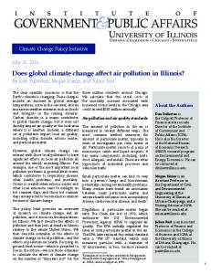
seven day average with a one day lag of each pollutant, but autocorrelation for the pollutants over time was a problem. In addition, their specification used a linear trend to account for all confounding factors, which almost certainly failed to account for important differences in weather and other factors that do not vary linearly over time. Hall et al (2003) examined the economic savings resulting from decreases in ozone-related school absences in California. They used the Regional Human Exposure Model (REHEX) to estimate exposure to air pollution and the Symptom-Valuation (SYMVAL) model, which uses concentration-response equations, to estimate the decrease in absences as a result. They regressed the changes in absences over two year periods on the changes in exposure as estimated by the REHEX model, and found approximately one less absence per year per child as a result of decreases in ozone levels. They estimated the economic value of the decrease in school absences due to ozone at approximately $75 per child from 1990-1992 to 1997-1999. However, this estimate only includes the benefit to the caregiver of their increased productivity; it does not include the reduced costs of medical care and long term health problems or the increased accumulation of human capital. Thus, the real benefit is likely much higher. Although the findings are interesting, the method used in this study is poorly described and does not make a compelling case that they have isolated reductions in ozone as a causal effect of the decline in absenteeism Most of the studies of school absenteeism and pollution have been conducted by medical researchers and focus on associations, not causal linkages. Taken as a whole, the results of epidemiological school absenteeism studies are inconclusive. However, O3 is consistently associated with school absences (see Figure 3.1). Park et al (2002) found that

15

PM10, SO2 and O3 were significantly associated with absenteeism, but NO2 was not. Gilliland et al (2000) found a strong association between O3 and absences due to respiratory illness, but no association with NO2 or PM10. Chen et al (2000) found CO and O3 to be significant predictors of absenteeism, but that absenteeism and PM10 were negatively correlated. Ransom and Pope (1991) found PM10 to be significantly associated with absenteeism and suggested the effects could linger for three to four weeks. In contrast, Ferris (1970) found that absences between schools were not statistically different despite large variations in pollution at the school’s locations. This limited absenteeism literature is inconclusive on issues of causation both because of the varying results and because some studies demonstrate nothing more than a simple correlation between pollution and absenteeism. Moreover, most of the schoolabsenteeism studies do not account for the fact that families sort in their choice of residence location based in part on pollution levels and associated factors, and thus are subject to problems of omitted variable bias. The overall inconclusiveness of the results and the disparate findings of the epidemiological literature regarding which pollutants are related to decreases in attendance highlight the gaps in the absenteeism literature and point to a need for more rigorous studies of the effects of pollution on attendance.

IV. Methodology I seek to improve upon previous studies of absenteeism by more thoroughly accounting for confounding factors that could bias the estimated effects of pollutants.

16

Authors

Title

Park et al

Association of Air Pollution with School Absenteeism Due to Illness

Gilliand et al

The Effects of Ambient Air Pollution on School Absenteeism Due to Respiratory Illness

Figure 3.1 Overview of Absenteeism Literature Method PM10 CO Daily absences regressed against daily pollutant levels using a Poisson regression Used two-stage timeseries model on daily absence count data over six months

Findings O3

NOX

SO2

Significantly positively related

N/A

Significantly positively related

No significant relationship

Significantly positively related

No significant relationship

N/A

Significantly positively related

No significant relationship

N/A

Elementary School Absenteeism and Air Pollution

Aggregate daily percentage absent for each grade regressed on several pollutants over two school years

Negatively correlated

Significantly positively related

Significantly positively related

N/A

N/A

Ransom, Michael and Pope, C. Arden

Elementary School Absences and PM10 Pollution in Utah Valley

Aggregate daily/weekly percentage absent for each grade regressed on several pollutants over 27 weeks

Significantly positively related

N/A

N/A

N/A

N/A

Ferris, Benjamin

Effects of Air Pollution on School Absences and Differences in Lung Function in First and Second Graders in Berlin, New Hampshire, January 1966 to June 1967

N/A

No significant relationship

N/A

N/A

N/A

No significant relationship

Hansen and Selte

Air Pollution and Sick-leaves

Logit specification of daily sick leave data over five years

Significantly positively related

N/A

N/A

No significant relationship

No significant relationship

Chen et. al

17

This section develops a model of the relationship between pollution and school absenteeism. Using the empirical model, I test if there is a causal link between pollution levels and missed days of school. I hypothesize that higher levels of pollution will lead to more negative health outcomes in children, perhaps due to the aggravation of asthma and other respiratory problems, thus causing students to miss more days of school than they would without the pollution. The fundamental impediment to the estimation of the causal effect of pollution is the sorting of families in their choice of residence, if families consider environmental quality or related factors that likely introduce correlations between other characteristics of a family and pollution. If these characteristics are also related to school absence rates, then pollution coefficients will be biased unless these other factors are accounted for. My approach takes advantage of panel data to control for likely confounding variables and identify the effects of pollution on absenteeism.

IV a. The Empirical Model Numerous factors affect health and absenteeism, including family background, community, weather, environment, etc. Equation (1) describes the unobserved propensity to be absent, A*, as a function of pollution, demographic characteristics, temperature and an error component.

(1) A*isypd = βpP sypd + βxXisy + βTTsypd + εisypd

18

Where A* is the unobserved propensity to be absent for student ‘i’ in school ‘s’ in year ‘y’ during attendance period ‘p’ on day ‘d’, P is a vector of pollutants, X is a vector of student demographic characteristics and T is the temperature and ε is the error term. Importantly, we do not observe A*, only whether a student is present or not. Let Aisypd =1 if the student is absent and 0 otherwise. Thus, Aisypd = 1 if A*isypd >0 and Aisypd =0 otherwise. In most specifications this binary nature of the data is ignored, however a group logit model is used to examine the sensitivity of the findings. Because the absence data is only available in six week blocks, I aggregate the variables by attendance period.3 Since all students in a school are exposed to the same level of pollution, I aggregate by school and grade for computational reasons. I use the average rate of absenteeism in a grade at a school during each six week attendance period as the dependent variable.

(2) Āgsyp = βpPsyp + βxX¯gsy + βTTsyp + ε¯gsyp

In equation (2), the average absentee rate is a function of pollution and a limited number of student demographics and weather variables. It is highly unlikely that this equation accounts for all confounding factors, which leads to the estimation of a biased coefficient. In the following specifications, I use panel data techniques to account for the primary remaining determinants of absenteeism with the inclusion of fixed effects. The key to generating causal estimates is that pollution, ‘P’, is uncorrelated with

3

X, the vector of individual characteristics, is not aggregated by attendance period because I only use students who are enrolled for all six periods.

19

the error, so it is important to account for unobservables correlated with both variations in pollution and variations in attendance.

(3) ε¯ gspy = µs + θy + γp + δg + πpy + λsp + νsy + ψgspy

In order to highlight key components of the error, equation (3) represents the error as a function of terms by school, period, year and grade, plus period-by-year, school-byperiod and school-by-year error terms. ψgspy is the random error term. Although there are many other possible interactions, the crucial components for this study are included in (3). The inclusion of school fixed effects accounts for the non-random sorting of students into schools. Because neighborhoods that are predominantly minority or low income are often located in areas with higher pollution, the schools serving these locations are also likely to be in high-pollution areas. Of course, students in these areas may miss more days of school than other students due to factors that are unrelated to pollution but are related to location choice. Adding school fixed effects accounts for heterogeneity among schools by using only within-school variation and accounting for differences between schools. The inclusion of school-by-year fixed effects accounts for changes in pollution and absenteeism over time. From year to year the composition of the student body may change, new administrators and teachers may arrive, redistricting can occur, school policies may change and the weather varies, all of which may affect the rate of absences and bias the coefficients. However, this is only a problem if pollution is also changing

20

systematically over time. Nonetheless, using school-by-year fixed effects accounts for year-to-year variation in addition to accounting for between-school variation. The inclusion of school-by-attendance period fixed effects account for within year seasonal differences by school. Weather and illness rates vary by school throughout the year and may be correlated with both attendance and pollution. For instance, children in grades one through eight are susceptible to non-pollution related illnesses which often affect many students at once. The patterns of these illnesses vary both by season and by school. They are also likely correlated with pollution since pollution varies by season too. For example, illnesses such as influenza and colds occur more frequently in the winter, when carbon monoxide peaks and other pollutants are at their lowest levels. Thus, the pattern of pollution variation may be correlated with season-related unobservables. To account for this and create a more comprehensive model, school-by-attendance-period fixed effects, which account for seasonal differences by school, are added to the schoolby-year fixed effects. The inclusion of period-by-year fixed effects accounts for state-wide seasonal differences over the years, including variation in the weather. A very important confounding factor that has so far been neglected is precipitation. When it rains, pollution levels drop dramatically as the air is cleared. Since damp weather makes children sick and staying indoors promotes the spread of illnesses, periods of more precipitation may also be correlated with more absences. Since weather moves in fronts, variations in weather are likely to be felt by the whole state. Adding period-by-year fixed effects accounts for such state-wide seasonal variation, including changes in precipitation.

21

Finally, the inclusion of a grade dummy variable accounts for differences in absenteeism between grades. Since this data spans grades one through eight, there may be differences in absence rates between children of different ages. For instance, younger children may miss more days do to illnesses, while older children may be more likely to skip school on a nice day. A grade dummy variable accounts for such systematic differences across grades. We have now accounted for all of the crucial components of the error term, resulting in the full fixed effects model:

(4) Āgsyp = βpPsyp + βxX¯gsy + βTTsyp + δ¯g + νsy + λsp + πpy + ε¯gsyp

which includes period, year and grade dummies, school-by-year, school-by-period and period-year fixed effects and an error term. This comprehensive specification leaves just school by year by attendance period variation in pollution. Although local weather and other factors may be contributing to this variation, I assume they are orthogonal to pollution. However, a potential problem is that the period-year term does not capture local weather variation which likely has a greater affect on attendance and pollution levels than state-wide weather patterns. One final issue is the nature of the dependent variable. Because a student is either absent or present, with no in between, each absence has only a binary outcome. Therefore, the absence rate varies between 0 and 1, violating the OLS assumption that errors are normally distributed. To check the sensitivity of the results to this assumption, I use a logit transformation similar to that used by Hansen and Selte. Weighted least

22

squares is used with the logit model and the dependent variable is transformed by 1/[(n*A)(1-A)] where n is the number of observations for each grade, school, year and period combination.

(5) log [Āgsyp/(1-Āgsyp)] = βpPsyp + βxX¯gsy + βTTsyp + δ¯g + πpy + ε¯gsyp

IV b. Measures of Pollution Because hourly pollution data is aggregated into six week blocks to match the attendance data, it is necessary to generate summary measures of pollution for that block of time. Since there may be a non-linear relationship between pollution and absences, and even the underlying relation between health and pollution is unclear, it is important to look at different measures of pollution. To account for different relationships, pollution is calculated based on the mean, median and 90th percentile of the aggregated hourly readings. The mean is the typical measure used in pollution studies, but the median and 90th percentile measures provide information on the number of days above or below a certain level. It may be that only very high levels of pollution affect attendance due to some sort of threshold (see below), in which case using the 90th percentile may generate stronger results. In addition, because the 90th percentile excludes most low pollution days (which in many cases may be caused by precipitation or weather event variables) it may be less sensitive to omitted variable biases. Each of the model specifications is run with all three pollution measures.

23

IV c. Thresholds and Harvesting To test the effects of any and all pollution on children, no thresholds were set for this analysis. Since children are more susceptible to pollution than adults, traditional thresholds – below which it is thought pollution does not cause adverse effects – are not necessarily accurate for them. This does not mean that a threshold is inappropriate for this study, but I did not have the information to determine one. Harvesting is another issue that often arises in pollution literature, but it is not a concern in this study. Harvesting occurs when an exogenous event (i.e. pollution) causes a major change in the frequency of the outcome, causing a large blip in the data. For instance, a particularly high ozone day may increase the mortality rate of elderly people the next day, making it seem as if the high ozone level is solely responsible for their deaths. However, they would likely have died within the next week anyhow, so the increase in pollution actually only shifted their deaths forward a few days. This is not an issue with school absences. A child missing school today because of pollution does not mean they would have missed school at a different point in time without the pollution. In this study, pollution directly causes the absence, not as a result of harvesting.

V. Data This paper uses panel data for the fifteen largest school districts in Texas – accounting for roughly 25% of the students in grades one through eight in the Texas public school system – for the academic years 1995-1996 through 2000-2001. Two different sources of data are used, one for pollution and one for attendance. Using the latitude and longitude of each school, pollution data is matched with schools. The

24

absence data is only available in aggregated six week attendance blocks, so the hourly pollution data is also aggregated into six week blocks based on the dates of the attendance periods. Since the school calendars vary from district to district, we include only those schools in districts for which the dates of the six week periods are known (see Table 5.1 for an example of period start and end dates). Table 5.1 Attendance Period Dates District Irving

Period 1 Start End

Period 2 Start End

Period 3 Start End

Period 4 Start End

Period 5 Start End

Period 6 Start End

8/14/95

9/25/95

11/6/95

1/8/96

2/20/96

4/8/96

9/22/95

11/4/95

12/15/95

2/16/96

4/4/96

V a. Attendance Data The school data in this paper comes from the UTD Texas Schools Project, which was conceived of and founded by John Kain. The database combines a number of different sources and contains data for all public school students and teachers in Texas, along with information about the schools themselves. In addition to information about absenteeism, we also use data on gender and ethnicity. Due to the way the data is collected, the number of days missed and the demographic characteristics of the students are aggregated over six week attendance blocks. For this study, individual attendance data is also aggregated by school, grade, and year to produce the grade-specific school average absentee rate for each six week block. The mean six week rate of absenteeism is 3.2%, while the 90th percentile is 7.1%.

V b. Pollution Data The pollution data comes from the Texas Commission on Environmental Quality (TCEQ), formerly the Texas Natural Resource Conservation Commission (TRNCC).

25

5/23/96

Individual monitors for each pollutant are set up all over the state and take hourly readings of the pollution levels at each location (with the exception of PM10, which is measured every sixth day). Over the years of this analysis, the numbers of monitors for each pollutant changed as some were taken on and off-line. Between the school years 1995-1996 and 2000-2001, the number of O3, NOx and weather monitors roughly doubled (to 72, 42 and 134 respectively). There were approximately 22 CO monitors throughout all six school years, and the number of PM10 monitors actually decreased from 31 to 21, likely due to an increase in the number of monitors measuring PM2.5 (see Table 5.2).

School Year 1995-1996 1996-1997 1997-1998 1998-1999 1999-2000 2000-2001

CO 23 23 19 22 22 22

Table 5.2 Number of Pollution Monitors NOx PM10 21 31 25 31 29 22 34 22 38 23 42 21

O3 45 47 54 59 68 72

Weather 68 93 36 110 97 134

Because the attendance data is only available in six-week blocks, the pollution data is also aggregated into six week blocks and the mean, median and 90th percentile level of each pollutant for each six week block are generated. As the following descriptive characteristics show, movements in the mean and median are quite similar, and though not shown a very similar pattern also holds for the 90th percentile (Figure 5.2 and Table 5.4). Pollutant levels vary across seasons and attendance periods, so there is variation in the amount of pollution at each school within a year (Figure 5.1). As noted above, ozone varies with temperature and peaks during the summer months. Ozone and PM10

26

are highest in the hotter months encompassed by attendance periods one, two and six, while carbon monoxide peaks during the winter in periods two, three and four. Nitrogen Oxide is fairly stable, with a slight peak in period two and a dip in period six. Table 5.3 shows the average pollutant levels over the entire six year period and Table 5.4 shows how the pollutant levels changed from year to year. Over the six year period studied, all four pollutants declined, reflecting the increasingly tough standards set by the EPA and localities. Mean levels of O3 declined by 6%, PM10 by 8%, NOx by 21% and CO by a substantial 42%. However, the overall decreases conceal year to year fluctuations (Figure 5.2). O3 and PM10 levels actually increased from the previous year in three of the six years, while most of the drop in NOx came in the final year of the study. Only CO showed an almost continuous decline in level over the six year period (with the exception of 1999-2000). Since O3 and PM10 consistently move in the same direction as temperature, it appears that the differences in pollution from year to year are primarily based on changes in average temperature. This highlights the importance of controlling for temperature in the analysis.

V. c Assigning Pollution to Schools To assign pollution to a school, the latitude and longitude of each school and pollution monitor were determined and the readings of the closest monitor for each pollutant were assigned to the school. Only monitors within 20 miles of a school were used. Of those within 20 miles, 50% of the monitors were within 3.7 miles of a school and 75% were within 5.9 miles. Only 1% of monitors were more than 12.9 miles from a school. Most of the school districts used in this study were in urban areas where there are more likely to be high concentrations of monitors. 27

Variable O3a COb PM10c NOd

Table 5.3 Pollution Averages: August 1995 –May 2001 (µg/m3) Mean Std. dev. 10th Percentile 90th Percentile 40.18 12.64 22.87 58.62 915.57 372.00 381.43 1674.25 25.48 6.51 13.70 39.95 34.49 7.64 18.25 52.26

Note: Mean/median refers to yearly mean/median of 6-week block’s means a c average 8-hour peak b average 8-hour peak measured every 6 days e average 1 hour average

d

average 21-hour peak

Table 5.4 School Mean & Median Pollutant Levels by Academic Year (µg/m3) 19951996199719981999Pollutant 1996 1997 1998 1999 2000 Mean O3a 41.80 36.51 39.84 40.12 43.82 Median O3a 41.63 35.83 39.40 38.66 42.82 Mean COb 1251.21 950.40 868.62 871.93 835.51 Median COb 1096.52 799.57 690.45 702.62 748.09 Mean PM10c 28.18 22.63 24.48 25.06 26.73 c Median PM10 26.45 20.65 22.52 23.31 25.71 d Mean NO 38.44 37.01 33.90 32.79 35.22 Median NOd 36.33 35.97 33.56 32.05 34.50 e Mean Temp . 18.65 17.76 17.91 19.69 19.75 Median Tempe. 19.47 18.14 18.17 20.02 20.17

20002001 39.11 38.30 720.09 593.25 25.92 23.66 30.20 29.14 17.87 18.09

*See notes from Table 5.3

28

0

0

mean of meanpm10 10 20

mean of meanoz8hrpk 20 40

30

60

0

0

10

mean of meanno21hrpk 20 30

mean of meanco8hrpk 500 1,000

40

1,500

Figure 5.1

Variation in Pollution by Six-Week Period (µg/m3 )

CO

1

1 2

2 3

3

NOx

4

4 5

5 6

6 1

1

2

2

3

O3 PM10

3

4 5 6

4 5 6

29

200 0

Temperature 200 0

199 9 -20 01

-20 00

40 35 30 25 20 15 10 5 0 -19 99

-19 98

-19 97

-19 96

200 0

199 9

199 8

199 7

199 6

199 5

200 0

199 9

-20 01

-20 00

-19 99

-19 98

-19 97

-19 96

-20 01

-20 00

-19 99

-19 98

-19 97

-19 96

O3

199 8

199 7

199 6

199 5

-20 01

-20 00

CO

-20 01

-20 00

-19 99

-19 98

-19 97

-19 96

199 9

199 8

199 7

199 6

199 5

45 40 35 30 25 20 15 10 5 0

200 0

199 9

199 8

199 7

199 6

199 5

-19 99

-19 98

-19 97

-19 96

1400 1200 1000 800 600 400 200 0

199 8

199 7

199 6

199 5

Figure 5.2 Annual Variation in School Pollutant Levels (µg/m3 ) Mean Median

30

PM10

25

20

15

10 5

0

NOX

21 18 15 12 9 6 3 0

30

However, monitor readings which are more distant from a school are noisier, since pollution disperses due to wind and other weather factors. This introduces measurement error which likely attenuates the coefficients. Moreover, the unadjusted standard errors are likely to be hetereoskedastic because errors are larger when the monitors are further away. To obtain a better understanding of the magnitude of these problems, a sensitivity check was performed by re-running the regressions using weighted least squares, with a weight of 1/distance (from the monitor to the school).

VI. Results The results present various specifications, culminating in the full fixed effects model which includes period-by-year, school-by-period and school-by-year fixed effects. Models using the mean, median and 90th percentile values of the pollutants are presented, as are models using weighted least squares. Although most of these models ignore the binary nature of the absence variable, a group logit specification is also presented. A discussion of the results, potential problems and future directions to take this research follows. Because the pollution data varies by school, period and year, while the observation sample varies by grade, school, pollution and year, robust standard errors clustered by school, period and year are reported for all of the following OLS and fixed effects regressions.4

4

These standard errors are almost certainly biased downward because many schools share the same pollution monitors.

31

VI a. Descriptive Statistics Prior to discussing the results, it is helpful to examine the sources of variation that are used in the following specifications. One potential problem with the fixed effect model is that after adding multiple fixed effects, very little variation may remain, exacerbating measurement error problems. To examine if this is a problem, Table 6.1 shows the variation left once fixed effects are added. Column one shows total variation of the pollution variables. Column two shows the residual variation after accounting for a school-by-period fixed effect. In most of the pollutants, the addition of the school-byperiod fixed effect causes the variation to drop by at least half. However, the variation only slightly decreases for ozone. Column three accounts for both school-by-year and school-by-period fixed effects, and column four shows the percent of the original variation that is left after accounting for both fixed effects. Ozone loses most of its variation with the addition of school-by-year fixed effects, resulting in the least amount of total variation of any of the pollutants with 10%. PM10 has the most, with 29%. Including both school-by-year and school-by-attendance period fixed effects accounts for most of the original variation, however there is still a considerable amount of variation left with which to isolate the effects of pollution.

VI b. Regression Results Tables 6.2- 6.4 show the results of the regressions of average absentee rate on all four pollutants, using different measures of pollution – mean, median and 90th percentile,

32

respectively. A variety of increasingly comprehensive specifications are shown, all of which include grade, year and period dummy variables. The first specification includes

Table 6.1 Variation Decomposition of Pollution Variables Residual Variation Accounting For: Total School by School by Year and Variation Attendance Period School by Attendance (mean) Fixed Effects Period Fixed Effects 159.86 149.37 16.13

O3

Percent of Original Variation Left 10.09

NOx

58.40

14.69

8.60

14.73

PM10

42.36

25.85

12.17

28.73

CO

138386.20

52914.98

20324.63

14.69

no demographic information, no temperature information, and no fixed effects. The second specification adds information on student demographic composition, including race and gender. Specification three includes average temperature over the six week block too. The fourth specification introduces the period-by-year interaction term. The fifth adds school-by-attendance period fixed effects, while the sixth alternatively adds school-by-year fixed effects. The seventh and final specification is comprehensive, including temperature, demographic variables, both school fixed effects terms and the period-year fixed effect. In the appendix, tables A.1-A.3 show the same specifications with each individual pollutant run separately in the model. Because the specifications using all pollutants and those using individual pollutants are fairly similar, it appears that multicollinearity does not affect the results. Although the pollutants are correlated, none of the correlation coefficients exceed 0.6.

33

Table 6.2 Estimated Effect of Mean Pollution Levels on the School Average Proportion of Days Students are Absent (Robust Standard Errors in Parentheses, 113,339 Observations)* Specifications 1 2 3 4 5 6 Variables O3 -0.319 -11.13 -4.08 -8.15 -8.14 -8.69 1.15 1.12 1.16 1.32 1.19 1.11

7 -3.52 1.17

NOX

0.681 1.33

-5.59 1.27

-6.35 1.27

-5.75 1.31

-2.47 1.18

2.25 1.42

4.37 1.26

PM10

-11.15 1.03

-11.15 1

-10.95 0.9923

-9.49 1.13

-5.96 1

-0.584 0.908

-5.89 0.905

CO

0.286 0.0217

0.239 0.0218

0.259 0.0219

0.313 0.023

0.228 0.0215

0.108 0.0246

0.168 0.0234

Average Temperature

n

n

y

y

y

y

y

Student Demographic Variables

n

y

y

y

y

y

y

n

n

n

n

y

n

y

n

n

n

n

n

y

y

n

n

n

y

y

y

y

School by Attendance Period Fixed Effects School by Year Fixed Effects Fully Interacted Period and Year Fixed Effect

* Each specification contains all pollutants Coefficients and standard errors are multiplied by 10^5

34

Table 6.3 Estimated Effect of Median Pollution Levels on the School Average Proportion of Days Students are Absent (Robust Standard Errors in Parentheses, 113,339 Observations)* Specifications 1 2 3 4 5 6 Variables O3 0.232 -9.78 -3.49 -7.19 -8.69 -7.02 0.96 0.933 0.958 1.18 0.875 0.872

7 -1.74 0.836

NOX

-2.89 1.21

-6.91 1.15

-6.07 1.15

-1.92 1.31

-1.38 1.03

1.35 1.15

2.61 0.997

PM10

-12.48 1.13

-13.09 1.09

-14.07 1.08

-7.07 1.39

-8.42 1.08

0.0627 1

-8.32 0.97

CO

0.326 0.0209

0.256 0.021

0.266 0.0211

0.267 0.0229

0.17 0.0208

0.103 0.227

0.0951 0.0215

Average Temperature

n

n

y

y

y

y

y

Student Demographic Variables

n

y

y

y

y

y

y

y

n

y

n

y

y

y

y

y

School by Attendance Period Fixed Effects n n n n School by Year Fixed Effects n n n n Fully Interacted Period and Year Fixed Effect n n n y * Each specification contains all pollutants Coefficients and standard errors are multiplied by 10^5

35

Table 6.4 Estimated Effect of 90th Percentile Pollution Levels on the School Average Proportion of Days Students are Absent (Robust Standard Errors in Parentheses, 113,339 Observations)* Specifications 1 2 3 4 5 6 Variables O3 0.175 4.66 4.35 1.62 5.45 4.97 0.753 0.724 0.746 0.902 0.918 0.678

7 2.88 0.86

NOX

-9.03 0.893

-10.9 0.869

-11.6 0.872

-7.33 1

-0.774 0.769

-5.73 0.925

4.76 0.843

PM10

-5.18 0.503

-4.87 0.486

-4.28 0.484

-5.46 0.622

-1.49 0.454

-1.6 0.412

-0.587 0.392

CO

.197 0.0123

0.15 0.0124

0.155 0.0123

0.194 0.0149

0.137 0.0123

0.112 0.0125

0.0755 0.0122

Average Temperature

n

n

y

y

y

y

y

Student Demographic Variables

n

y

y

y

y

y

y

n

n

n

n

y

n

y

n

n

n

n

n

y

y

n

n

n

y

y

y

y

School by Attendance Period Fixed Effects School by Year Fixed Effects Fully Interacted Period and Year Fixed Effect

* Each specification contains all pollutants Coefficients and standard errors are multiplied by 10^5

The results vary by specification and measure of pollution. However, CO is consistently positive and significant, while PM10 is consistently negative (and almost always significant). By comparison, O3 and NOx vary more across specifications. 36

Comparing Tables 6.2 and 6.3, one sees that the results when using the mean and the median are very similar. The results when using the 90th percentile are somewhat different. Most of the coefficients are larger, O3 is consistently positive and significant, and, in the full specification, PM10 also ceases to be significant when using the 90th percentile as the measure. There are several reasons to think that the 90th percentile may provide a better measure of pollution than the mean or the median. If children are more susceptible to pollution at higher levels – i.e. there is some sort of threshold – than the 90th percentile makes the most sense as an aggregate of pollution data. In addition, as discussed above, the 90th percentile may mitigate some omitted variable biases. This may be especially important in the case of O3 because it is highly affected by temperature and precipitation. Since the 90th percentile mitigates these biases by only utilizing variation in highpollution days, it might provide a better estimate of the true effect of O3, suggesting it is a significant and positive causal factor of student absenteeism. NOx also varies by specification, but is positive and significant only in the most comprehensive specification, when using all three measures of pollution. None of the previous studies described in Table 3.1 found a significant effect from NOx; more work is needed to make sure that this is not a spurious result. However, the changes in NOx highlight the difference that the addition of one fixed effect term can make to a specification. Adding school fixed effects (specifications 5, 6 and 7) changes the nature of the data. Because school fixed effects account for variation between schools, leaving only variation within a school, the data is no longer cross-sectional. The inclusion of school-by-attendance period and school-by-year fixed

37

effects produced large changes in the estimated coefficients. Part of the change is likely due to accounting for heterogeneity between schools, because within-school variation is likely less affected by some of the omitted variables discussed above than across-school variation. However, the addition of year and period fixed effects are also important. The school-by-year fixed effect accounts for changes in weather from year to year, in addition to major changes in school policy or composition that may have a large effect on attendance. The school-by-attendance period fixed effect accounts for seasonal variation in weather and behavior. Each of these terms contributes to a substantial increase in coefficients, suggesting they both account for omitted variables. However, their effects are not consistent. O3 becomes much larger with the introduction of the school-by-year fixed effect, while PM10’s coefficient rises more when school-byattendance period fixed effects are added. CO is slightly more affected by the introduction of school-by-year, while the NOx coefficient increases almost equally with the addition of either. Including a period-by-year term which accounts for precipitation and other statewide seasonal weather variations, something not done in many previous studies, also made most of the coefficients more positive (or less negative). Because rain causes pollution levels to drop dramatically, and likely also increases absences, it is an important omitted variable which was biasing the coefficients in earlier specifications. Throughout different specifications using different measures of pollution, PM10 is consistently negative and only in the full specification using the 90th percentile is it insignificant. However, these unexpected results are not that surprising. In the absenteeism literature surveyed above (Table 3.1), three studies found PM10 to be

38

significantly positively related to absenteeism, two found it to be insignificant, and one found it to be negatively correlated. Since PM10 is not an actual pollutant but rather a classification for certain sized particles, it reflects the trends of different pollutants (and other particles) at the same time. Since different pollutants have different seasonal peaks, the overall correlation between PM10 and attendance may be difficult to isolate. In addition, it is important to consider that there is quite a bit more measurement error involved with the PM10 data than the other pollutants. While the other pollutants are measured in hourly intervals, PM10 is only measured every sixth day. Over a six week interval, there are only about seven measures of PM10, which likely reduces the precision of the results. The magnitude of effect varies by pollutant. Using the full specification with the 90th percentile measure, a 1µg/m3 increase in NOx causes a .0048 percentage point increase in the absentee rate, a 1µg/m3 increase in O3 causes a .0029 percentage point increase and a 100µg/m3 increase in CO increases the absenteeism rate by .0076 percentage points.5 Given that the school year consists of 180 days, effects of these magnitudes imply that 1/100 children miss an additional 1.4 days of school per attendance period due to a 100µg/m3 increase in CO, an additional 0.86 days due to a 1µg/m3 increase in NOx and an additional 0.52 days due to a 1µg/m3 increase in O3. Finally, Table 6.5 provides a sensitivity check of the model, using the 90th percentile as the measure of pollution levels. The unweighted specification is the same as the seventh specification in table 6.4 – the full fixed effects model. The next two columns use weighted least squares to weight the model. The second specification weights it by 5

Because the mean level of CO varies from 1250 to 720 over the six year period, while the mean levels of O3 and NOx vary from 41 to 39 and from 38 to 30, respectively, a 100µg/m3 increase provides a better sense of the magnitude of the impact of CO.

39

enrollment, while the third weights it by distance. Because larger schools have more observations and thus a larger sample size, the variance of the error is likely to be smaller and weighting by enrollment accounts for this source of heteroskedasticity. Likewise, as discussed above, there is a problem of heteroskedasticity due to the noise that occurs when assigning pollution to schools. The variance of the error term is likely inversely related to the distance between the school and the pollution monitor. To account for this, the specification is weighted by 1/distance. The weighted least squares changes little. Both weights reduce the size of the coefficients a little, and O3 ceases to be significant (although remains positive) when weighted by 1/distance. This lack of major differences in the three specifications shows that the model is robust to different weights. The group logit model (Appendix Table A.4) is run using the 90th percentile of pollution and no fixed effects to test if the basic model is affected by the violation of OLS. Because the group logit coefficients represent log odds, a coefficient above one means pollution increases absences, while a result below one means pollution decreases absences. Using all of the pollutants, the results are similar to specification one in Table 6.4, suggesting that ignoring the binary nature of the absence data does not introduce serious problems. The standard errors are not clustered in the group logit transformation, which explains the high significance of the coefficients. All in all, these additional regressions suggest that heteroskedasticity and measurement error are not major problems.

40

Table 6.5 Sensitivity Checks - Full Fixed Effects Model (Robust Standard Errors in Parentheses, 113,339 Observations) Unweighted Specification 2.88 0.86

Weighted by Enrollment 3.02 0.871

Weighted by 1/Distance 1.06 1.05

NOX

4.76 0.843

4.54 0.0843

3.67 1.11

PM10

-0.587 0.392

-0.558 0.4

-0.136 0.452

CO

0.0755 0.0122

0.0643 0.0119

0.089 0.0142

y

y

y

y

y

y

y

y

y

y

y

y

y

y

y

O3

Average Temperature Student Demographic Variables School by Attendance Period Fixed Effects School by Year Fixed Effects Fully Interacted Period and Year Fixed Effects

* All specifications use the 90th percentile as the measure of pollution and contain all pollutants Coefficients and standard errors are multiplied by 10^5

VII. Conclusions

41

The results of this study indicate that two pollutants – O3 and CO– are causally linked to an increase in student absenteeism. The effects of NOx are more ambiguous and there is no evidence that PM10 increases absenteeism rates. This study also shows that the 90th percentile may be a better measure of pollution in absenteeism studies, perhaps because it overcomes threshold problems and accounts for weather-related omitted variable biases. Likewise, including a fixed effect term that accounts for seasonal variation in weather appears to reduce omitted variable bias. The current school absenteeism literature is inconclusive, and this study suggests both that certain pollutants do have an adverse effect on attendance and that previous studies were likely affected by omitted variable biases. An important issue is whether the magnitude of the effect is significant in an economic sense, which depends in large part on the link between absenteeism and human capital accumulation. This relationship is likely to be nonlinear because one or two additional absences may not matter much, but a larger number may really affect a student’s ability to keep up in class. If there is a subset of students that are particularly affected by pollution, such as children with asthma or other respiratory problems, they may be the ones who are accumulating significantly less human capital over time. This suggests two potential improvements on this analysis for future studies. In this study it was only possible to identify average effects, but if it was possible to isolate children with respiratory problems then one could test if they are experiencing more absences than their peers as a result of pollution, and thus accumulating less human capital. In addition, studies to quantify the cost of reduced school attendance in terms of

42

long-term human capital accumulation would make it possible to estimate the economic costs of school days missed due to pollution. One way to evaluate the actual costs is to look at the effects of pollution on student test scores. While this analysis sought to examine the causal link between air pollution and school attendance, future studies could investigate the link between pollution and student achievement. There is some literature on pollution as it relates to absenteeism, but there is almost none on air pollution and achievement. In a recent paper, Pastor et al (2004) found that “environmental hazard indicators are associated with diminished school-level academic performance…” but little work has been done beyond that. In considering the absenteeism related costs imposed by pollution, it is important to evaluate both current lost productivity to parents that occurs when a child misses a day of class, and also the costs to human capital investment which might be better measured by test scores. There are additional improvements to this study that would provide a more accurate and detailed analysis of air pollution’s effects on absenteeism. An analysis of this scale with individual level daily data (instead of six week aggregated blocks) would provide a better measure of the effects of pollution. Because this data is aggregated over six week blocks, I lose day-to-day variation which reduces the statistical power of the analysis. Daily data would provide more variation and also allow for daily dummy variables (such as the day before a holiday) in order to account for some of the nonpollution related absences. Creating a better model of pollution and weather is another way in which this study could be improved. Obviously precipitation is an important variable that should be

43

considered in the specifications of future analyses, but creating a better measure of school’s exposure to pollution is another potential improvement. A better measure of pollution would account for the direction of the wind, current weather, and other such factors which influence how pollution is dispersed between the monitor and the school. In addition, using multiple nearby monitors to determine the level of pollution at the school could provide a more accurate measure. Pollution is a negative externality, and ascertaining the external costs it imposes is necessary before an efficient level can be determined. The costs to reduce pollution are often very high, including building new factories, changing the way cars are built, and potentially finding new sources of energy. From an economic perspective, such costly endeavors are only worthwhile if they confer an equal or greater economic benefit in reduced health costs, increased productivity and better quality of life. The adverse effects of pollution on school attendance shown by this study suggest that pollution does reduce productivity and human capital investment. Future work to quantify these costs and determine other long-term costs of pollution are necessary to determine an efficient level of pollution.

44

Appendix Table A.1 Estimated Effect of Individual Mean Pollution Levels on the School Average Proportion of Days Students are Absent (Robust Standard Errors in Parentheses, 114,425 Observations for PM10, 124,360 Observations for O3, 123,532 Observations for CO, 119,893 Observations for NOx)* Specifications 1 2 3 4 5 6 7 Variables O3 -1.34 -1.66 -8.53 -4.18 -4.73 -1.42 -8.39 0.82 0.81 0.892 0.958 1 0.744 1.07 NOX

-2.42 1.01

-7.79 0.973

-9.36 0.999

-5.66 1.02

-0.868 1.06

-0.0792 1.09

6.4 1.07

PM10

-6.13 0.855

-8.89 0.84

-9.24 0.84

-5.12 0.929

-4.62 0.967

-1.51 0.74

-5.1 0.865

CO

0.262 0.0165

0.224 0.0167

0.202 0.0175

0.288 0.0171

0.204 0.0179

0.0483 0.0182

0.109 0.0192

n

n

y

y

y

y

y

n

y

y

y

y

y

y

n

n

n

n

y

n

y

School by Year Fixed Effects

n

n

n

n

n

y

y

Fully Interacted Period and Year Fixed Effect

n

n

n

y

y

y

y

Average Temperature Student Demographic Variables School by Attendance Period Fixed Effects

* Each specification contains results from separate regressions of individual pollutants Coefficients and standard errors are multiplied by 10^5

45

Appendix Table A.2 Estimated Effect of Individual Median Pollution Levels on the School Average Proportion of Days Students are Absent (Robust Standard Errors in Parentheses) * Specifications 1 2 3 4 5 6 Variables O3 -1.35 -8.47 -4.44 -5.24 -3.07 -7.08 0.696 0.683 0.747 0.786 0.732 0.626

7 -2.69 0.699

NOX

-4.49 0.967

-8.17 0.916

-9.15 0.932

-5.26 0.979

-0.0738 0.939

-0.0925 0.975

3.93 0.89

PM10

-10.74 1.2

-12.47 0.983

-13.77 0.977

-6.49 1.13

-7.72 1.04

-1.09 0.845

-7.82 0.916

CO

0.237 0.0176

0.226 0.0176

0.212 0.0184

0.305 0.018

0.168 0.0178

0.0377 0.0177

0.0445 0.0182

n

n

y

y

y

y

y

Average Temperature

Student Demographic Variables n y y y y y y School by Attendance Period Fixed Effects n n n n y n y School by Year n n n n n y y Fixed Effects Fully Interacted Period and Year Fixed Effect n n n y y y y * For sample size, see Table A1 Each specification contains results from separate regressions of individual pollutants Coefficients and standard errors are multiplied by 10^5

46

Appendix Table A.3 Estimated Effect of Individual 90th Percentile Pollution Levels on the School Average Proportion of Days Students are Absent (Robust Standard Errors in Parentheses)* Specifications 1 2 3 4 5 6 7 Variables O3 -0.958 -0.232 -0.355 5.9 2.82 -2.83 3.36 0.536 0.536 0.588 0.696 0.818 0.496 0.705 NOX

-4.96 0.716

-8.21 0.691

-9.55 0.724

-6.75 0.732

1.1 0.707

-1.88 0.699

8.196 0.71

PM10

-2.86 0.431

-4.12 0.422

-3.75 0.424

-4.97 0.558

-0.686 0.447

-1.16 0.36

-0.166 0.379

CO

0.14 0.00877

0.121 0.00888

0.111 0.00943

0.139 0.00983

0.129 0.0106

0.0559 0.00924

0.0863 0.0102

Average Temperature

n

n

y

y

y

y

y

Student Demographic Variables

n

y

y

y

y

y

y

School by Attendance Period Fixed Effects n n n n y n y School by Year Fixed Effects n n n n n y y Fully Interacted Period and Year Fixed Effect n n n y y y y * For sample size see table A1 Each specification contains results from separate regressions of individual pollutants Coefficients and standard errors are multiplied by 10^5

47

Appendix Table A.4 Group Logit Transformation of Full Model (Standard Errors in Parentheses, 126,300 Observations)*

Variables O3

90th Percentile 1.002952 0.0001511

NOX

0.9980754 0.0001247

PM10

0.9980541 0.0000902

CO

1.000031 2.11E-06

Average Temperature

y

Student Demographic Variables

y

School by y Attendance Period Fixed Effects School by Year y Fixed Effects Fully Interacted y Period and Year Fixed Effects * Each specification was run with all pollutants using the 90th percentile measure of pollution

48

Bibliography Bridges to Sustainability and Mickey Leland National Urban Air Toxics Research Center. 2003. “Final Report: Assessment of Information Needs for Air Pollution Health Effects Research in Houston, Texas.” Feb. 17, 2003. Chay, Kenneth and Greenstone, Michael. 2001. “Air Quality, Infant Mortality, and the Clean Air Act of 1970.” NBER Working Paper #w10053, August 2001. Chay, Kenneth and Greenstone, Michael. 2000. “Does Air Quality Matter? Evidence from the Housing Market.” NBER Working Paper #w7442, December 2000. Chen, Lei et al. 2000. “Elementary School Absenteeism and Air Pollution.” Inhalation Toxicology. 12: 997-1016 Currie, Janet and Neidell, Matthew. “Air Pollution and Infant Health: What if We Can Learn From California’s Recent Experience?” NBER Working Paper 10251 Dixon, Jane. 2002. “Kids Need Clean Air: Air Pollution and Children’s Health.” Family & Community Health. 24(4): 9-26. Dockery, Douglas et al. 1993. “An Association Between Air Pollution and Mortality in Six U.S. Cities.” The New England Journal of Medicine. 329 (24): 1753-1759 EPA – 2004. Air Emissions Trends – Continuing Progress Through 2003. http://www.epa.gov/airtrends/econ-emissions.html – 2004. Six Principal Pollutants. http://www.epa.gov/airtrends/sixpoll.html – 2003. Executive Summary of 2003 National Air Quality and Emissions Trends Report. http://www.epa.gov/air/airtrends/aqtrnd03/pdfs/chap1_execsumm.pdf – 1998. 1998 National Air Quality and Emissions Trends Report. http://www.epa.gov/air/airtrends/aqtrnd98/ Ferris, Benjamin. 1970. “Effects of Air Pollution on School Absences and Differences in Lung Function in First and Second Graders in Berlin, New Hampshire, January 1966 to June 1967.” American Review of Respiratory Disease. 102: 591-606. Gilliland, Frank et al. 2001. “The Effects of Ambient Air Pollution on School Absenteeism Due to Respiratory Illness.” Epidemiology. 12: 43-54. Hall, Jane, Brajer, Victor and Lurmann, Frederick. 2003. “Economic Valuation of OzoneRelated School Absences in the South Coast Air Basin of California.” Contemporary Economic Policy. 21 (4): 407-417. Hansen, Anett and Selte, Harald. 2000. “Air Pollution and Sick-Leaves,” Environmental and Resource Economics. 16: 31-50,

49

Houghton, F et al. 2003. “The Use of Primary/National School Absenteeism as a Proxy Retrospective child Health Status Measure in an Environmental Pollution Investigation.” Public Health. 117: 417-423. Linn, William et al. 1996. “Short-Term Air Pollution Exposures and Responses in Los Angeles Area Schoolchildren.” Journal of Exposure Analysis and Environmental Epidemiology 6 (4):449-472 Lippman, Morton. “Environmental Toxicants.” Van Nostrand Reinhold, New York. 1992. Makino, Kuniyoshi. 2000. “Association of School Absences with Air Pollution in Areas around Arterial Roads.” Journal of Epidemiology. 10 (5): 292-299. Park, Hyesook et al. 2002. “Association of Air Pollution with School Absenteeism Due to Illness.” Archives of Pediatric & Adolescent Medicine. 156: 1235- 1239. Pastor, Manuel et al. 2004. “Reading, Writing and Toxics: Children’s Health, Academic Performance, and Environmental Justice in Los Angeles.” Environment and Planning C: Government and Policy. 22: 271-290. Ponka, Antii. 1990. “Absenteeism and Respiratory Diseases among Children and Adults in Helsinki in Relation to Low-Level Air Pollution and Temperature.” Environmental Research. 52: 34-46. Ransom, Michael and Pope, C. Arden. 1992. “Elementary School Absences and PM10 Pollution in Utah Valley.” Environmental Research. 58: 204-219. Reyes, Jessica. “The Impact of Prenatal Lead Exposure on Infant Health.” Working Paper, 2002. Reyes, Jessica. “Environmental Policy as Social Policy? The Impact of Childhood Lead Exposure on Crime.” Working Paper, 2003. Samet et al. 2000. “Fine Particulate Air Pollution and Mortality in 20 U.S. Cities, 19871994.” The New England Journal of Medicine. 343 (24):1742-1749. Sunyer et al. 1997. “Urban Air Pollution and Emergency Admissions for Asthma in Four European Cities: The APHEA Project.” Thorax. 52: 760-765

50