Digital Image Processing for Image Enhancement and Information Extraction

Summary Digital image processing plays a vital role in the analysis and interpretation of Remotely sensed data. Especially data o b t a i ned from Satellite Remote Sensing, which is in the digital form, can best be utilised with the help of digital i mage processing. Image enhancement and information extraction are two important components of digital image p r o c e s s i ng. Image enhancement techniques help in improving the visibility of any portion or feature of the image s u p p r e s sing the information in other portions or features. Information extraction techniques help in obtaining the statistical information about any particular feature or portion of the image. These techniques are discussed in detail and illustrated in this article.

1. IMAG E-PROCESSING OVERVIEW Digital Image P rocessing (DIP ) involves the modification of digital data for improving the image qualities with the a i d of computer. The processing helps in maximising clarity, sharpness and details of features of interest towards i n fo r ma t i o n e xt raction and further analysis. This form of remote sensing actually began in 1960s with a limited n u mber of researchers analysing airborne multispectral scanner data and digitised aerial photographs. However, it w a s n o t u n t i l the launch of Landsat-1, in 1972, that digital image data became widely available for land remote sensing applications. At that time not only the theory and practice of digital image processing was in its infancy but a l s o t h e cost of digital computers was very high and their computational efficiency was far below by present s t a ndards. Today, access to low cost and efficient computer hardware and software is commonplace and the source o f d i g i t a l i ma g e data are many and varied. The digital image sources range from commercial earth resources s a tellites, airborne scanner, airborne solid-state camera, scanning micro-densitometer to high-resolution video camera. D i g i t a l i ma g e processing is a broad subject and often involves procedures which can be mathematically complex, but central idea behind digital image processing is quite simple. The digital image is fed into a computer a n d c omputer is programmed to manipulate these data using an equation, or series of equations and then store the results of the computation for each pixel (picture element). These results form a new digital image that may be displayed or recorded in pictorial format or may itself be further manipulated by additional computer programs. The p o s s i b l e fo r ms o f the digital image manipulation are literally infinite. The raw digital data when viewed on the display will make it difficult to distinguish fine features. To selectively enhance certain fine features in the data and to remove certain noise, the digital data is subjected to various image processing operations. Image-processing me t h o d s ma y b e grouped into three functional categories: these are defined below together with lists of typical processing techniques. 1

2

3

I m a g e Restoration compensates for data errors, noise and geometric distortions introduced during the scanning, recording, and playback operations. a. Restoring periodic line dropouts b. Restoring periodic line striping c. Filtering of random noise d. Correcting for atmospheric scattering e. correcting geometric distortions I m a g e Enhancement alters the visual impact that the image has on the interpreter in a fashion that improves the information content. a. Contrast enhancement b. Intensity, hue, and saturation transformations c. Density slicing d. Edge enhancement e. Making digital mosaics f. P roducing synthetic stereo images Inf ormation Extraction utilizes the decision-making capability of the computer to recognize and classify pixels on the basis of their digital signatures, a. P roducing principal-component images b. P roducing ratio images c. Multispectral classification d. P roducing change-detection images

Image enhancement and information extraction methods are described and illustrated in the following sections.

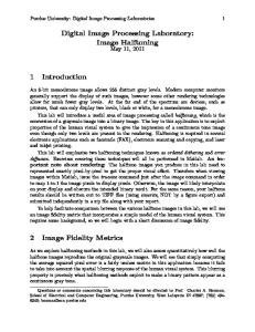
2. IMAG E ENHANCEMENT E n h a n c e me n t is the modification of an image to alter impact on the viewer. Generally enhancement distorts the original digital values; therefore enhancement is not done until the restoration processes are completed. 2.1 Contrast Enhancement There is a strong influence of contrast ratio on resolving power and detection capability of images. Techniques for improving image contrast are among the most widely used enhancement processes. The sensitivity range of any remote sensing detector is designed to record a wide range of terrain brightness from black basalt plateaus to white sea beds under a wide range of lighting conditions. Few individual scenes have a brightness range that utilizes the fu l l s e n s i tivity range of these detectors. To produce an image with the optimum contrast ratio, it is important to u t ilize the entire brightness range of the display medium, which is generally film. Figure 1 shows the typical h i s togram of the number of pixels that c o r r e s p ond to each DN of an image with no mo d i fi cations of original DNs. The central 92 p e r c e n t of the histogram has a range of DNs fr o m 49 to 106, which utilizes only 23 percent of the available brightness range [(106 - 49)/256 = 2 2 .3%]. This limited range of brightness values accounts for the low contrast ratio of the o r iginal image. Three of the most useful methods of contrast enhancement are described in the following sections. 2 .1 .1 Linear Contrast Stretch: The simplest c o ntrast enhancement is called a linear contrast s t r e t c h . A DN value in the low end of the o r iginal histogram is assigned to extreme black a n d a value at the high end is assigned to e xt reme white. In this example the lower 4 p e rcent of the pixels (DN < 49) are assigned to b l ack, or DN = 0, and the upper 4 percent (DN > 106) are assigned to white, or DN = 255. The remaining pixel values are distributed linearly b e t w e en these extremes, as shown in the e n h anced histogram of Figure 2. The improved c o n t r ast ratio of the image with linear contrast s t retch will enhance different features on the ma p . Most of the image processing software display an image only after linear stretching by default. For colour images, the individual bands were stretched before being combined in colour. Th e linear contrast stretch greatly improves the contrast of most of the original brightness values, but there is a loss of contrast at the extreme high and low end of DN values. In comparison to the overall contrast improvement, t h e s e contrast losses at brightness extremes are acceptable unless one is critically interested in these elements of the scene. B e c a u se of the flexibility of digital methods an investigator could, for example, cause all DNs less the 106 to become black (0) and then linearly stretch the remaining high DNs greater than 105 through a range from 1 through 2 5 5 . Th i s e xt r e me stretch would enhance the contrast differences within the bright pixels at the expense of the remainder of the scene. 2 .1 .2 N onlinear Contrast Stretch: Nonlinear contrast enhancement is made in different ways. Figure 3 illustrates a unif orm distribution stretch (or histogram equalization) in which the original histogram has been redistributed t o p r oduce a uniform population density of pixels along the horizontal DN axis. This stretch applies the greatest contrast enhancement to the most populated range or brightness values in the original image. In Figure 3, the middle range of brightness values are preferentially stretched, which results in maximum contrast. The uniform distribution stretch strongly saturates brightness values at the sparsely populated light and dark tails of the original histogram. The resulting loss of contrast in the light and dark ranges is similar to that in the linear contrast stretch but not as severe. A G aussian stretch (Fig. 3a) is a nonlinear stretch that enhances contrast within the tails of the histogram. This s t r e t c h fi t s t he original histogram to a normal distribution curve between the 0 and 255 limits, which improves contrast in the light and dark ranges of the image. This enhancement occurs at the expense of contrast in the middle grey range.

A n important step in the process of contrast enhancement is for the user to inspect the original histogram and d e t e rmine the elements of the scene that are of greatest interest. The user then chooses the optimum stretch for his n e e d s . Experienced operators of image processing systems bypass the histogram examination stage and adjust the brightness and contrast of images that are displayed on a screen. For some scenes a variety of stretched images are required to display fully the original data. It should be noted that contrast enhancement should not be done until other processing is completed, because the stretching distorts the original values of the pixels. 2.2 Intensity, Hue and Saturation Transf ormations 255 Th e a d d itive system of primary colours (red, green, and blue, or RGB s y stem) is well established. An alternate approach to colour is the i n t e nsity, hue and saturation system (IHS), which is useful because it A p r e s ents colours more nearly as the human observer perceives them. Blue Th e IHS system is based on the colour sphere (Figure 4) in which the v e rtical axis represents intensity, the radius is saturation, and the 0 c i r c u mference is hue. the intensity (I) axis represents brightness variations and ranges from black (0) to white (255): no colour is associated with this axis. Hue (H) represents the dominant wavelength o f c o l o u r. Hue values commence with 0 at the midpoint of red tones a n d i n crease counterclockwise around the circumference of the sphere to conclude with 255 adjacent to 0. Saturation (S) represents the purity of colour and ranges from 0 at the centre of the colour sphere to 255 at 0 t h e circumference. A saturation of 0 represents a completely impure colour, in which all wavelengths are equally represented and which the e y e w i l l perceive a shade of grey that ranges from white to black depending on intensity. Intermediate values of saturation represent Figure 4. Intensity, Hue and Saturation colour coordinate system. Colour at point A has the pastel shades, whereas high values represent purer and more intense values: I=195, H=75 and S=135. colours. The range from 0 to 255 is used here for consistency with the eight-bit scale; any range of values (0 to 100, for example) could as well be used as IHS coordinates. Buchanan (1979) describes the IHS system in detail. When any three spectral bands of a sensor data are combined in the RGB system, the resulting colour images typically lack saturation, even though the bands have been contrast-stretched. The under-saturation is due to the high d e g r e e o f correlation between spectral bands. High reflectance values in the green band, for example, are accompanied by high values in the blue and red bands, so pure colours are not produced. To correct this problem, a method of enhancing saturation was developed that consists of the following steps: 1

Tr a n s fo r m a n y t h ree bands of data from the RGB system into the IHS system in which the three component images represent intensity, hue, and saturation. The equations for making this transformation are described below.

I = R+ G+B ;

H = G -B ; I - 3B

S = I - 3B I

2

Th e i ntensity image is dominated by albedo and topography. Sunlit slopes will have high intensity values (bright tones), Water has low values, Vegetation has intermediate intensity values, as do most of the rocks. In the hue image, the low DNs are used to identify red hues in the sphere (Figure 4), Vegetation has intermediate t o light grey values assigned to the green hue. The lack of blue hues is shown by the absence of very bright tones. The original saturation image will be very dark because of the lack of saturation in the original data. Only the shadows and GREEN, H=1 rivers are bright, indicating high saturation for these features.

3

Apply a linear contrast stretch to the original saturation image. Note the overall increased brightness of the enhanced image. Also note the improved discrimination between terrain types.

4

Tr ansform the intensity, hue, and enhanced saturation images from t h e IHS system back into three images of the RGB system. These e n h a n c e d RGB images were used to prepare the new colour c o mposite image of, which will be a significant improvement over t h e original image. In the IHS version, note the wide range of colours and improved discrimination between colours.

Th e fo llowing description of the IHS transformation is a summary of the work of R. Hayden (Short and Staurt, 1982). Figure 5 shows

0.5

BLUE H=2

2.5

Figure 5. Diagram showing the relationship between the RGB and IHS systems

H=0 RED H=3

g r a p h i c ally the relationship between the RGB and IHS systems. Numerical values may be extracted from this d i a g r a m fo r e xpressing either system in terms of the other. In Figure 5 the circle represents a horizontal section through the equatorial plane of the IHS sphere (Figure 4), with the intensity axis passing vertically through the plane o f t h e diagram. The corners of the equilateral triangle are located at the position of the red, green, and blue hues. H u e c hanges in a counterclockwise direction around the triangle, from red (H = 0), to green (H = 1), to blue (H = 2 ) , a n d a gain to red (H = 3), Values of saturation are 0 at the centre of the triangle and increase to a maximum of 1 a t t h e corners. Any perceived colour is described by a unique set of IHS values; in the RGB system, however, different combinations of additive primaries can produce the same colour. The IHS values can be derived from R G B values through the transformation equations explained above for the interval 0 < H < 1, extended to I < H < . After enhancing the saturation image, the IHS value are converted back into RGB images by inverse equations. Th e I H S t r a n s fo rmation and its inverse are also useful for combining images of different types. For example a digital radar image could be geometrically registered IRS optical data. After the optical bands are transformed into I H S values, the radar image data may be substituted for the intensity image. The new combination (radar, hue, and enhanced saturation) can then be transformed back into a RGB image that incorporates both radar and optical data. 2.3 Density Slicing D e n s i t y slicing converts the continuous grey tone of an image into a series of density intervals, or each c o r r e s p o n d i n g to a specified digital range D. Slices may be displayed as areas bounded by contour lines. This technique emphasizes subtle grey-scale differences that may be imperceptible to the viewer. 2.4 Edge Enhancement M o s t i n t e r p r eters are concerned with recognizing linear features in images such as joints and lineaments. Geographers map manmade linear features such as highways and canals. Some linear features occur as narrow lines against a background of contrasting brightness; others are the linear contact between adjacent areas of different b r i g h t n e s s . I n a ll cases, linear features are formed by edges. Some edges are marked by pronounced differences t h a t may be difficult to recognize. Contrast enhancement may emphasize brightness differences associated with s o me l i n e a r features. This procedure, however, is not specific for linear features because all elements of the scene are enhanced equally, not just the linear elements. Digital f ilters have been developed specifically to enhance edges in images and fall into two categories: directional and nondirectional. 2.4.1 Nondirectional Filters: Laplacian f ilters are nondirectional filters as they enhance linear features having a l most any orientation in an image. The exception applies to linear features oriented parallel with the direction of fi l t e r mo v e me nt; these features are not enhanced. A typical Laplacian filter (Figure 6 A) is a kernel with a high c e n t r a l v alue, 0 at each corner, and -1 at the centre of each edge. The Laplacian kernel is placed over a three-bythree array of original pixels (Figure 6 A) and each pixel is multiplied by the corresponding value in the kernel. The n i n e r esulting values (four of which are 0 and four are negative numbers) are summed. The resulting value for the fi l t e r k e r nel is combined with the central pixel of the three-by three data array, and this new number replaces the original DN of the central pixel. For example, the Laplacian kernel is placed over the array of three-by three original pixels indicated by the box in Figure 6 A. When the multiplication and summation are performed, the value for the filter kernel is 5. The central pixel in the original array (DN = 40) is combined with the filter value to produce the n e w value of 45, which is used in the filtered data set (Figure 6 B). The kernel moves one column of pixels to the right, and the process repeats until the kernel reaches the right margin of the pixel array. The kernel then shifts back t o t h e l e ft ma r g i n , drops down one line of pixels, and continues the same process. The result is the data set of filtered pixels shown in Figure 6 B. In this filter data set, the outermost column and line of pixels are blank because they cannot form central pixels in an array.

50

50

50

50

45

45

45

50

50

50

50

50

50

50

55

55

55

55

0

-1

0

50

50

50

50

45

45

45

50

50

50

50

50

50

50

55

55

55

55

-1

4

-1

A 50

50

50

50

45

45

45

50

50

50

50

50

50

50

55

55

55

55 B

0

-1

0

50

50

50

50

45

45

45

50

50

50

50

50

50

50

55

55

55

55

A. Original Data Set and Laplacian Filter Kernel

A

50

50

55

40

45

40

55

50

50

50

50

50

45

60

55

55

55

50

50

55

40

45

40

55

50

50

50

50

50

45

60

55

55

55 B

50

50

55

40

45

40

55

50

50

50

50

50

45

60

55

55

55

B. Filtered Data Set

C. P rofile of the Original data along A-B.

D. P rofile of the Filtered data along A-B. Figure 6. Nondirectional Edge Enhancement using a Laplacian Filter Th e e ffe c t of the edge-enhancement operation can be evaluated by comparing profiles A-B of the original and the filtered data (Figure 6 C,D). The original data has a regional background value of 40 that is intersect by a darker, n o r t h - t e n d i n g l i n eament and background, with a contrast ratio of 40/35 or 1.14. In the enhanced profile the c o n t r a s t ratio is 45/30 or 1.50, which is a marked enhancement. In addition the image of the original lineament, w h i c h w a s t h r e e pixels wide, has been widened to five pixels in the filtered version, which further enhances its appearance.

In the eastern portion of the original data set (Figure 6 A), the background values (40) change to values of 45 along a n o r t h - t ending linear contact. In an image this contact would be a subtle tonal lineament between brighter and darker surfaces. The original contrast (45/40 = 1.13) is enhanced by 27 percent in the filter image (50/35 = 1.43). A ft e r the value of the filter has been calculated and prior to combining it with the original central data pixel, the c a l c u lated value may multiplied by a weighting f actor. The weight factor can be less than 1 or greater than 1 in order to diminish or to accentuate the effect of the filter. The weighted filter value is then combined with the central original pixel to produce the enhanced image.

2 .4.2 Directional Filters: Directional filters are used to enhance specific linear trends in an image. A typical directional filter (Figure 7 A) consists of two kernels, each of which is an array of three by three pixels.

Cos A *

-1

0

1

-1

0

1

+ Sin A

1

1

1

0

0

0

-1

-1

-1

= Filter value

*

-1

0

1

A. Directional Filter Kernel 50

50

50

50

50

50

50

50

50

50

50

45

50

50

50

50

45

45

A 50

50

50

45

45

45 B

50

50

45

45

45

45

50

45

45

45

45

45

B. Original Data. Edge direction is N45 oE(-)

A

0

0

0

0

-7

0

0

0

-7

-14 -14

0

0

-7

-14 -14

0

-7

-14 -14 -7

-7

-14 -14

-14 -14 -7

-14

-7 0 B

-7

0

0

0

0

0

C. Kernel Values

50 50 50 50 43 36 50 50 50 43 36 31 50 50 43 36 31 38 A 50 43 36 31 38 45 B 43 36 31 38 45 45 36 31 38 45 45 45 D. Sum of Original data and Kernel Values

Figure 7. Edge Enhancement using a Directional Filter Th e l e ft k e r n e l i s mu ltiplied by the cos A, where A is the angle, relative to north, of the linear direction to be enhanced. The right kernel is multiplied by sin A. Angles in the northeast quadrant are considered negative; angles i n the northwest quadrant are positive. The filter can be demonstrated by applying it to a data set (Figure 7 B) in which a brighter area (DN = 40) is separated from a darker area (DN = 35) along a total lineament that trends northeast (A = -45 o). The profile A-B shows the brightness difference (DN = 5) across the lineament. Th e fi l t e r i s demonstrated by applying it to the array of nine pixels shown by the box over the original data set (Figure 7 B). The sequence of operations is as follows: 1 2

P lace the right filter kernel over the array of original pixels and multiply each pixel by the corresponding filter value. When these nine resulting values are summed, the filter result is 10. D e t e r mine the sine of the angle (sin - 45 o = -0.71) and multiply this by the filter result (-0.71 x 10) to give a filter value of -7.

3 4

5

P lace the left filter kernel over the pixel array and repeat the process; the resulting value is -7. S u m the two filtered values (-14); This value replaces the central pixel in the array of the original data. when steps 1 through 4 are applied to the entire pixel array, the resulting filtered values are those shown in the array and profile of Figure 7 C. Th e fi l t e red values for each pixel are then combined with the original value of the pixel to produce the array and profile of Figure 7 D.

The contrast ratio of the lineament in the original data set (40/35 = 1.14) is increased in the final data set to (40/21 = 1 .9 0 ) , w h i ch is a contrast enhancement of 67 percent. As shown in profile A-B, the original lineament occurs across an interface only one pixel wide; the enhanced lineament has an image four pixels wide. An alternate way to express this operation is to say that the filter has passed through the data in a direction normal to the specified lineament direction. In this example the filter passing through direction is N45 oW. In addition to e n h a ncing features oriented normal to this direction of movement, the filter also enhances linear features that trend o b l i q u e l y t o the direction of filter movement. As a result, many additional edges of diverse orientations are enhanced. The directionality of the filter may also be demonstrated by passing the filter in a direction parallel with a linear trend. As a result these fractures appear subdued, whereas north and northeast-tending features are strongly enhanced. 2.5 Making Digital Mosaics M o s a i c s o f images may be prepared by matching and splicing together individual images. Differences in contrast a n d t one between adjacent images cause the checkerboard pattern that is common on many mosaics. This problem c a n b e l argely eliminated by preparing mosaics directly from the digital CCTs, as described by Bernstein and F e r n e y h ough (1975). Adjacent images are geometrically registered to each other by recognizing ground control points (GCP s) in the regions of overlap. P ixels are then geometrically adjusted to match the desired map projection. The next step is to eliminate from the digital file the duplicate pixels within the areas of overlap. Optimum contrast stretching is then applied to all the pixels, producing a uniform appearance throughout the mosaic. 2.6 Producing Synthetic Stereo Images Ground-control points may be used to register image pixel arrays to other digitized data sets, such as topographic maps. This registration causes an elevation value to be associated with each image pixel. With this information the computer can then displace each pixel in a scan line relative to the central pixel of that scan line. P ixels to the west of the central pixel are displaced westward by an amount that is determined by the elevation of the pixels. The same p r o c e d u r e determines eastward displacement of pixels east of the central pixel. The resulting image simulates the p a r a l l a x o f a n a e rial photograph. The principal point is then shifted, and a second image is generated with the parallax characteristics of the overlapping image of a stereo pair. A synthetic stereo model is superior to a model from side-lapping portions of adjacent Landsat images because (1) Th e vertical exaggeration can be increased and (2) The entire image may be viewed stereoscopically. Two d i s a d v a ntages of computer synthesised stereo images are that they are expensive and that a digitized topographic map must be available for elevation control. S i mp s o n et al. (1980) employed a version of this method to combine Landsat images with aero-magnetic maps (in which the contour values represent the magnetic properties of rocks). The digitized magnetic data are registered to t h e Landsat band so that each Landsat pixel has an associated magnetic value. The stereoscopic transformation is t h e n u sed to produce a stereo pair of Landsat images in which magnetic values determine the vertical relief in the s t e r e o model. Elevated areas represent high magnetic values and depressions represent low magnetic values. The stereo model enables the interpreter to compare directly the magnetic and visual signatures of the rocks.

3. INFORMATION EXTRACTION Image restoration and enhancement processes utilize computers to provide corrected and improved images for study by human interpreters. The computer makes no decisions in these procedures. However, processes that identify and e xt r a c t i n fo rmation do utilize the computer's decision-making capability to identify and extract specific pieces of i n fo r ma tion. A human operator must instruct the computer and must evaluate the significance of the extracted information.

X2

3.1 Principal-Component Images F o r a n y pixel in a multispectral image, the DN values are commonly highly correlated from band to band. This c o r r e l ation is illustrated schematically in Figure 8, which plots digital numbers for pixels in TM bands 1 and 2. The elongate distribution pattern of the data points indicates that as brightness in band 1 increases, brightness in band 2 also increases. A three-dimensional plot (not illustrated) of three bands, such as 1,2 and 3, would show the data points in an elongate ellipsoid, indicating correlation of the three bands. This correlation means that if the reflectance of a pixel in one band (IRS band 2, for example) is known, one can p r e d ict the reflectance in adjacent bands (IRS bands 1 and 3 ). The correlation also means that there is much r e d u ndancy in a multispectral data set. If this redundancy could be reduced, the amount of data required to describe a multispectral image could be compressed.

IRS Band 1 Digital Numbers

X1

Figure 8. Scatter P lot of IRS Band 1 (X1 axis) and Band 2 ( X 2 axis) showing Correlation between these Bands. Th e P incipal-components transformation was used to generate a new Coordinate System (Y 1, Y 2)

Th e p r i n c ipal-components transformation, originally known as the Karhunen-Loeve transformation (loeve, 1955), i s u s e d to compress multispectral data sets by calculating a new coordinate system. For the two bands of data in Figure8, the transformation defines a new axis (y 1) oriented in the long dimension of the distribution and a second axis (y 2) perpendicular to y 1. The Mathematical operation makes a linear combination of pixel values in the original coordinate system that results in pixel values in the new coordinate system:

y 1 = α11 x1 + α 12 x2 y 2 = α21 x1 + α 22 x2 where (x1, x2) are the pixel coordinates in the original system; (y1, y2) are the coordinates in the new system; and α 11, α 1 2 , α 2 1 and α 22 are constants. In Figure 8, note that the range of pixel values for y 1 is greater than the ranges for either of the original coordinates, x1 or x2 and that the range of values for y2 is relatively small. The same principalc o mp o n e n t s t r a nsformation may be carried out for multispectral data sets consisting of any number of bands. Additional coordinate directions are defined sequentially. Each new coordinate is oriented perpendicular to all the previously defined directions and in the direction of the remaining maximum density of pixel data points. For each p i xe l , n e w DNs are determined relative to each of the new coordinate axes. A set of DN values is determined for each pixel relative to the first principal component. These DNs are then used to generate an image of the first p r i n cipal component. The same procedure is used to produce images for the remaining principal components. The p r e c eding description of the principal-components transformation is summarized from Swain and Davis (1978) and additional information is given in Moik (1980). A n y t h r e e principal-component images can be combined to create a colour image by assigning the data that make u p e a c h i mage to a separate primary colour. In summary, the principal-components transformation has several advantages: 1 Most of the variation is a multispectral data set is compressed into one or two P C images 2 Noise may be relegated to the lesson related P C images, and 3 Spectral differences between materials may be more apparent in P C images than in individual bands.

3.2 Ratio Images Ratio images are prepared by dividing the DN in one band by the corresponding DN in another band for each pixel, s t r e t c hing the resulting value, and plotting the new values as an image. A total of 15 ratio images plus an equal number of inverse ratios (reciprocals of the first 15 ratios) may be prepared from six original bands. In a ratio image t h e b l a c k and white extremes of the grey scale represent pixels with the greatest difference in reflectivity between t h e t w o s p e c t r a l b ands. The darkest signatures are areas where the denominator of the ratio is greater than the n u me r a t o r . C onversely the numerator is greater than the denominator for the brightest signatures. Where d e n o mi n a t o r a n d numerator are the same, there is no difference between the two bands. For example, the spectral reflectance curve shows that the maximum reflectance of vegetation occurs in IRS band 4 (reflected IR) and that reflectance is considerably lower in band 2 (green). The ratio image 4/2, results when the DNs in band 4 are divided by the DNs in band 2. The brightest signatures in this image correlate with the vegetation. L i k e P C i mages, any three ratio images may be combined to produce a colour images by assigning each image to a s e p a r a t e primary colour. The colour variations of the ratio colour image express more geologic information and h a v e g r e a t er contrast between units than do the conventional colour images. Ratio images emphasize differences

i n slopes of spectral reflectance curves between the two bands of the ratio. In the visible and reflected IR regions, the major spectral differences of materials are expressed in the slopes of the curves; therefore individual ratio images a n d r a t i o c o l our images enable one to extract reflectance variations. A disadvantage of ratio images is that they s u p p r ess differences in albedo; materials that have different albedos but similar slopes of their spectral curves may be indistinguishable in ratio images. Ratio images also minimize differences in illumination conditions, thus suppressing the expression of topography. I n a d d i tion to ratios of individual bands, a number of other ratios may be computed. An individual band may be divided by the average for all the bands, resulting in normalized ratios. Another combination is to divide the d i fference between two bands by their sum; for example, (band 4 - band 3)/(band 4 + band 3) of IRS. Ratios of this type are used to study the crop condition and crop yield estimation. 3.3 Multispectral Classif ication F o r e ach pixel in IRS or Landsat TM image, the spectral brightness is recorded for four or seven different wavelength bands respectively. A pixel may be characterized by its spectral signature, which is determined by the r e l a t i v e reflectance in the different wavelength bands. Multispectral classification is an information-extraction process that analyzes these spectral signatures and then assigns pixels to categories based on similar signatures. By plotting the data points of each band at the centre of the spectral range of each muti spectral band, we can g e n e r a t e c l u s t er diagram. The reflectance ranges of each band form the axes of a three-dimensional coordinate s y s t e m. P lotting additional pixels of the different terrain types produces three-dimensional clusters or ellipsoids. The surface of the ellipsoid forms a decision boundary, which encloses all pixels for that terrain category. The volume inside the decision boundary is called the decision space. Classification programs differ in their criteria for defining the decision boundaries. In many programs the analyst is able to modify the boundaries to achieve optimum r e s u l t s . F o r t h e sake of simplicity the cluster diagram is explained with only three axes. In actual practice the computer employs a separate axis for each spectral band of data: four for IRS and six or seven for Landsat TM. O n c e t h e b o u n daries for each cluster, or spectral class, are defined, the computer retrieves the spectral values for e a c h pixel and determines its position in the classification space. Should the pixel fall within one of the clusters, i t i s c l a s s ified accordingly. P ixels that do not fall within a cluster are considered unclassified. In practice, the c o mp u t e r c a l culates the mathematical probability that a pixel belongs to a class; if the probability exceeds a designated threshold (represented spatially by the decision boundary), the pixel is assigned to that class. There are two major approaches to multispectral classification viz., Supervised classification and unsupervised classification. In Supervised classif ication, the analyst defines on the image a small area, called a training site, which is r e p resentative of each terrain category, or class. spectral values for each pixel in a training site are used to define t h e d e c i s ion space for that class. After the clusters for each training site are defined, the computer then classifies all the remaining pixels in the scene. In Unsupervised classif ication , the computer separates the pixels into classes with no direction from the analyst. 3.3.1 Classif ication Algorithms Va r i o u s c l a s s i fi c a tion methods may be used to assign an unknown pixel to one of the classes. The choice of a p a r t i c u l a r classifier or decision rule depends on the nature of the input data and desired output. P ARAMETRIC c l a s s ification algorithm assumes that the observed measurement vectors Xc obtained for each class in each spectral band during the training phase of the supervised classification is Gaussian in nature. Nonparametric classification a l g o r i t h m ma k es no such assumption. It is instructive to review the logic of several of the classifiers. The P arallelepiped, Minimum distance and Maximum likelihood decision rules are the most frequently used classification algorithms. (a) The parallelepiped classif ication algorithm: This is a widely used decision rule. It is based on simple Boolean and/or logic. Training data in n spectral bands a r e u s e d i n performing the classification. Brightness values from each pixel of the multispectral imagery are used to produce an n-dimensional mean vector,

M c = [µc1, µc2, µc3, ........ , µcn ] w i th µck being the mean value of the training data obtained for class c in band k out of m possible classes as p r e v i o u s ly defined. Sck is the standard deviation of the training data class c in band k out of m possible classes. Using a one standard deviation threshold a parallelepiped algorithm assigns the pixel in class c if, and only if

µck - Sck