public goods has conventionally been specified with the Walrasian type. In this study, it is argued thatforpublicgoods, demand should be more properly specified with a Marshallian- type function in which tax share a function of the quantity demanded of public goods. First, theoretical reasoning why the demand function for public goods must be of the Marshallian type is discussed, and the demandfunction of this specification is developed and estimated to evaluate its merits.
Demand function for is Abstract
THE PUBLIC GOOD DEMAND FUNCTION: TAX SHARE AS A DEPENDENT VARIABLE U-JIN JHUN University of New JANG H. YOO State
York at
Oswego
Virginia Commonwealth University
for public goods has conventionally Demand function with the Walrasian In most studies
been
specified type. (e.g., Bergstrom and Goodman, 1973; Borcherding and Deacon, 1972), public expenditure (quantity demanded) is a function of the tax share (price) together with other &dquo;quantity&dquo; variables like population, income, grant-in-aid, race, and unemployment. This type of public good demand function seems to be theoretically inadequate and empirically incomplete, because the demand function should be the total price that individuals in the society are willing to pay at each possible quantity of public goods. Therefore, it is more realistic to say that a given quantity demanded for public goods determines price (i.e., tax share). Changing the hypothesis this way, we can first avoid the so-called simultaneous bias in the demand estimation, and second we can remedy the unreality of using tax share as an independent variable which is endogenous or &dquo;unpredictable&dquo; in its nature. This paper is an attempt to argue that for public goods, demand should
PUBLIC FINANCE QUARTERLY, Vol. 6 @ 1978 Sage Publications, Inc.
No. 3, July 1978
[277]
[278] be more properly specified with a Marshallian-type function in which tax share is a function of the quantity demanded of public goods together with some &dquo;cost&dquo; variables. First, theoretical reasonings why the demand function for public goods must be of the Marshallian type will be discussed, and then the demand function of this specification will be developed and estimated to evaluate its merits and demerits. Those who specify the public good demand with a Walrasian-
type function put their theoretical basis on the voluntary exchange
theory first developed by Bowen (1943), then followed by Downs (1957), Arrow (1963), and Buchanan and Tullock (1962). In this theory, it is implicitly assumed, among other things, that (1) all individuals in the community actually vote to express their preferences for public goods, (2) the cost of whatever amount of public good to be produced will be divided equally among all citizens, (3) produced public goods will be shared equally among the members of the society (equal benefit shares), (4) the price of the public goods is set so that the quantity demanded is equal to the quantity supplied, and (5) a constant cost of public good production is assumed so that average and marginal costs are equal and constant. Based on these assumptions, the relationship between the government and the taxpayer is treated as a voluntary one, and taxes are viewed as prices paid for government services. This theoretical basis is vulnerable to criticism. Unlike private goods, public goods available to and demanded by different individuals cannot be adjusted according to their respective tastes. The amount of the public goods, which is measured usually in terms of their money costs, must be set by a single decision applicable jointly to all the members of the society. This amount of money the society as a whole is willing to give up to obtain successive units of public goods may be derived by adding the marginal rates of substitution for all the members of the society. This total marginal rate of substitution curve approximates the total demand curve for public goods. This demand curve is different from the demand for private goods in that the former is obtained by adding prices various individuals are willing to pay at each pos-
[279]
sible quantity of public goods. The process of deriving the total demand for public goods clearly suggests that a given quantity demanded determines price. The political theory of the expenditure-tax mix decision process explains that each individual, motivated by self-interest, votes for politicians who have the most desirable mix of expenditures and taxes and certain proposed programs the voter prefers. This theory is based on somewhat unrealistic assumptions. In reality, voters rarely can participate in expenditure decisions with knowledge of the tax share, since the price each individual will have to pay is determined after the amount of public good production is determined. For example, in municipal financing, the property tax rate is derived after the value of property is assessed and the total expenditure needed for each locality is determined. EMPIRICAL FRAMEWORK
Since empirical researchers are dealing with collected data of actual public goods produced and prices charged, the shape of the demand function will depend on the supply function of public goods. Ironically, it is variability in the supply function which enables us to measure the demand relations. In regard to a supply function, we can make three assumptions. First, if we specify that the supply of public goods is an increasing function of tax rates, then, based on the sample data, we will not be able to distinguish between the demand and supply functions. Only when we bring another explanatory variable (e.g., shared revenue) into the supply function may the demand function be identified and will we have a simultaneous equation model. Second, if we assume that the supply function is infinitely price elastic, then we can formulate a demand function with a single equation based on the analysis that the price of a public good determines the quantity demanded rather than the supply function. But this causal relationship is not acceptable for reasons stated in the previous section.
[280]
Thus, the most realistic assumption is that the supply curve of public goods in the short run is perfectly inelastic, and prices are determined by quantity supplied. We can also assume that the demand curve remains relatively stable, while the vertical supply curve shifts in either direction (Figure 1). These assumptions provide us with the following major advantages: (1) the specification of the public good demand function becomes more realistic, using tax share as a dependent variable and quantity (i.e., per capita expenditure) as an independent variable, (2) we can avoid a simultaneous-bias problem, (3) since the demand function is specified as a price equation, we can introduce into the equation as additional arguments such &dquo;cost-related&dquo; factors as city
Figure
1
[281]
employee/ population and the general economic condition which cannot be included in the conventional demand equation. In what follows, we try to test empirically the following hypotheses to support our foregoing arguments: (1) income elasticity of public good demand is very low, which indicates that the demand curve remains relatively stable, (2) the Marshallian demand function behaves better than the Walrasian in terms of R2, t-values, and so on, (3) income and price elasticities are more consistent in the Marshallian function compared to what other economists have found using the Walrasian function.
MODELS AND DATA
To find the price and income elasticity, we started with the conventional Walrasian form of a nonlinear demand function such as
where q = per capita total expenditure, p = tax share of the median income class, y = per capita median income, A = some constant, and 6 is the disturbance term; a and /3 are the price and income elasticity, respectively, and a < 0, /3 > 0. Using p as a dependent variable, we have:
where A’ = ( 1A)l/a, and c-’ = ( 1f) l/a. We estimated basically equation 2 using the OLS method. To refine the e term, we add on the right-hand side some cost variables that affect the price level such as public employee divided by
population (E/ P) and the general economic use various quantities for q, such as:
also
condition (7r). We
[282] ql
=
q2
=
q3
=
q4
=
capita total expenditures other than education and welfare expenditures (they are excluded because of federal supports of these expenditures.) per capita highway services per capita police and fire service per capita sanitation and sewage services. per
Data on p, q, y, E/ P, and 7r were collected for six major cities in the United States: Buffalo, Cleveland, Denver, Detroit, Houston, and New York. These cities were chosen with a view to similarity in terms of their population density and industrial characteristics. Data for each city cover 1953-1973 (21 time-series observations). The- data sources are listed in the Appendix. The actual equation we estimated is in the logarithmic form of equation 2 plus other scale variables, i.e.:
TABLE 1
Regression
Results of
Equation 3-Pooled Data
1 Number of observations =126 2 Values m the parenthesis are student t-values &dquo;Statistically significant at the 596 level
[283] TABLE 2
Comparison
a
Based
on
among Studies of B-D, B-G, and J-Y
1962 cross-section data aggregated at the’state level pooled cross-section data at the state level,and the national level 1953-1973 time series data pooled m six major cities
b Based on 1962 c
Based
on
We estimated equation 3 using pooled data. The estimation method was based upon Kmenta’s pooling cross-section and time-series data (Kmenta, 1971: 508-514).~Table 1 summarizes the estimated coefficients. From the estimated values in Table 1, we can compute « (price elasticity) and /3 (income elasticity) and compare these with the estimation of Borcherding and Deacon (1972) and Bergstrom and Goodman (1973). Table 2 summarizes this. It is realized that the comparisons among the three studies are limited because of differing data bases and model specifications. However, our results are much more consistent in that all the price elasticities are negative and between -1.5 and -2.2, and all the income elasticities are positive and consistently small (between 0.13 and 0.28), whereas Borcherding and Deacon’s and Bergstrom and Goodman’s results are inconsistent in signs and values of elasticities. Our estimation clearly supports the idea we presented earlier, i.e., (1) the demand curve has been fairly stable without shifting
[284] or down as shown by low values of income elasticities, (2) there is no simultaneous bias problem in estimating the public good demand curve, (3) the Marshallian type of demand curve including (E/ P) and 7r variables in the demand function behaves much more consistently in terms of the elasticity values, (4) all the statistical values (R2 and t-statistics) are generally better than B-D or B-G equations.
up
CONCLUSION The Walrasian demand function based upon the voluntary exchange theory is not appropriate for public good demand in both the theoretical and the empirical sense. In reality, voters cannot participate in expenditure decisions not knowing the price level, since that is determined only after the amount of public good production is fixed. We started with the hypothesis that the Marshallian type of demand curve with quantity and cost factors as independent variables would work better in terms of econometric criteria and the plausibility of values obtained. This hypothesis has been accepted, and other empirical aspects are satisfactory in general.
NOTES 1. A demand function is called either the Marshallian or the Walrasian type depending upon which market adjustment mechanism the model is based. That is, in the Walrasian demand theory, quantity demanded is determined by the level of prices (i.e., Q = f (P)), whereas in the Marshallian case, demand price depends upon the quantity of the good (i.e., P = f (Q)). However, since we deal with public goods whose quantities and prices are determined not by the market adjustment mechanisms but by a certain single public decision applicable to all in the society, we simply borrow the terms "Walrasian"and "Marshallian" only for referring to their respective functional forms without being concerned about the adjustment mechanisms or stability problems.
[285] 2. This method is based upon the
assumption
that there exists
heteroskedasticity
2 Σe / (n-k-1) from indi2 cross-sectionally and autocorrelation time-wise. Thus, we find s vidual runs for the six cities, and we also obtain the autocorrelation coefficient δ t-1 for each city. Thus, we deflate all the observation values for each city by 2 (Σe e-1)/ ) t (Σe 2 and δ to find the pooled coefficients. its s =
=
REFERENCES ARROW, K. J. (1963) Social Choice and Individual Values. New York: John Wiley. BARR, J. and O. A. DAVIS (1966) "An elementary political and economic theory of the
expenditures of local governments."
Southern Econ. J. 33
(October):
149-165.
BERGSTROM, T. C. and R. P. GOODMAN (1973) "Private demands for public goods." Amer. Econ. Rev. 63 (June): 280-296. BORCHERDING, T. E. and R. T. DEACON (1972) "The demand for the services of nonfederal
governments."
Amer. Econ. Rev. 62
(December);
891-901
BOWEN, H. (1943) "The interpretation of voting in the allocation of economic resources."
Q. J. of Economics 58 (November): 27-48. BUCHANAN, J. M. and G. TULLOCK (1962) The Calculus of
Consent. Ann Arbor: Univ. of Michigan Press. DOWNS, A. (1957) An Economic Theory of Democracy. New York: Harper. KMENTA, J. (1971) Elements of Econometrics. New York: Macmillan.
APPENDIX 1. For population and per capita income between 1953-1973, we&dquo; used the various issues of Survey of Buying Power, from Sales Management.
2. For public employment per 1,000 population, we used the various issues of City and County Data Book, Department of Commerce, Washington, D.C., and Local Government in Metropolitan Areas, Department of Commerce, Washington, D.C., and Survey of Buying Power from Sales Management. 3. For expenditures data, we used the various issues of City Government Finances, Department of Commerce, Washington, D.C. Also, Finances of Municipalities and Township Governments, Department of Commerce, Washington, D.C.
[286] 4. The general economic condition was collected from the various issues of Business Condition Digest, Department of Commerce, Washington, D.C.
U-Jin Jhun is Assistant Professor of Economics at the State University of New York at Oswego. His recent publications have appeared In the Journal of Economic Development and the Nebraska Journal of Economics and Business.
Yoo is an Assistant Professor in the Department of Economics at Virginia Commonwealth University. His publications have appeared in the Journal of Economic Development, Journal of International Studies, and Kyklos, and he is author (with Ott and Ott) of Macroeconomic Theory and (with F. Ott) New York City’s Financial Crisis: Can the Trend Be Reversed?
Jang H.