International Review of Electrical Engineering (I.R.E.E.), Vol. 5. n. 2, pp. 785-792

ِCircular Antenna

Array Synthesis Using Fuzzy Genetic Algorithm M. Bousahla1, B. Kadri2, F.T. Bendimerad1

Abstract – This paper presents a rigorous synthesis of circular arrays of printed antennas using a hybrid fuzzy-genetic algorithm. Fuzzy logic based controllers are applied to fine-tune dynamically the crossover and mutation probability in the genetic algorithms, in an attempt to improve the algorithm performance. The FGA approach is compared with the Standard Genetic Algorithm(SGA). Included synthesis example clearly demonstrates that while the SGA approach gives satisfactory solutions for the problem, the FGA method usually performs significantly better. Copyright © 2009 Praise Worthy Prize S.r.l. - All rights reserved. Keywords: Fuzzy genetic algorithms, population diversity measurements, circular antennas array, synthesis, fuzzy controller.

Nomenclature pm pc D Dg

mutation probability crossover probability whole diversity of population gene diversity of population

D gw

D gb

gene inner diversity gene outer diversity

Di

individual diversity of population

Dib

individual outer diversity individual inner diversity individuals average fitness

Diw

Pi P f

f max Number

M l N

ϕi

k0 Ri

( Ai , α i ) Etot (r, θ, φ) E (θ , φ ) di d av Sll max fitness

average fitness of the population average fitness of the current population. fitness of the optimal individual frequency of the largest fitness value that is not changed number of individuals in the population length of string representing the individual number of element in array. angular position of ith Antenna wave number. distance between the ith patch and the observation complex excitation coefficients of the ith patch total radiated field of an array radiation pattern of one patch ith sample of the pattern in the beam region average value in the beam region highest sidelobe level fitness function of an individual

Manuscript received January 2007, revised January 2007

I.

Introduction

The printed antennas array aroused an interest growing during these last years, in particular in the mobiles communications fields and the monolithic structures, where the radiating elements and the phaseconverters are integrated in the same substrate. They also find applications in the space techniques to ensure a specific or partial terrestrial cover, like in the military and civil field. This is mainly due to the unique feature of microstrip antennas; which are, namely, low in profile, compact in structure, light in weight, conformable to non planar surfaces, easy and inexpensive for mass production. The array association of several printed elements allows in addition an improvement of their performances, to accomplish a very particular functions, such as : scanning and beam steering, jamming rejection, adaptive detection, autoadaptativity, carrying out of various radiation patterns, the directivity pattern and polarization control, …etc. The circular array, in which the radiating elements are placed on circular rings, is an array of very great practical interest. These applications are multiple: radars, sonar, terrestrial and space navigation and much of other systems [1-2]. The application of genetic algorithms GAs as optimization tools for the design of antennas has been an active field of search in the past decade [3-4]. They have roved to be a useful and powerful alternative to traditional optimization techniques [5-7] when handling with multidimensional, multimodal optimization problems, and their success is related to versatility, robustness and ability to optimize non differentiable cost function [3,8-9]. The performances of the genetic algorithm is correlated to directly with its careful selection of parameters. It is possible to destroy an high fitness Copyright © 2007 Praise Worthy Prize S.r.l. - All rights reserved

M. Bousahla, B. Kadri, F.T. Bendimerad

individual when a large crossover probability is set. The performance of the algorithm would fluctuate significantly. For a low crossover probability, sometimes it is hard to obtain better individuals and does not guarantee faster convergence. High mutation introduces too much diversity and takes longer time to get the optimal solution. Low mutation tends to miss some nearoptimal points. Adaptive genetic algorithms, which dynamically adapt selected control parameters or genetic operators during the evolution, have been built to avoid the premature convergence problem and improve GA behaviour. One of the adaptive approaches is the parameter setting techniques based on the use of fuzzy logic controllers (FLCs), the fuzzy genetic algorithm (FGA) [8-11]. In this paper we develop the synthesis of the complex radiation pattern of a circular antenna array with probe feed by optimizing amplitude excitation coefficients, the desired radiation pattern is specified by a narrow beam pattern with a beam width of 8 degrees and a maximum side lobe levels of -30dB pointed at 0°. The simulation results obtained while applying FGAs are compared, in the same conditions, with those obtained by the standard genetic algorithms SGAs. In section 2 we present the design method of the proposed optimization technique, the design of a fuzzy controller is discussed to adjust crossover and mutation probabilities according to the population diversity measurements and the best fitness individual. The synthesis problem of a circular antenna array with rectangular cells using FGAs by optimization of the complex excitation coefficients is presented in section 3. In section 4: numerical results for a circular array using both the SGAs and FGAs are presented to compare the performances obtained while introducing fuzzy techniques in GAs. Finally, some conclusions are drawn in section 5.

II.

Fuzzy Genetic Algorithms

Genetic algorithm was proposed by Holland in the 1970s [3], which is an optimization algorithm simulating natural evolution. Although GA becomes very famous with its global searching, parallel computing, better robustness, and not needing differential information during evolution. GAs include three primary genetic operators: selection, crossover and mutation. Selection embodies the principal of ‘Survival of the fitness’. The attention of crossover is to recombine genetic material of parents to form their offspring and to reach the new regions in search space [10-11]. The role of mutation in GAs has been that of restoring lost or unexpected genetic material into population to prevent premature convergence of the GA to sub-optimal solutions. However, GA has also some demerits, such us poor local searching, premature converging as well as slow convergence speed.

Copyright © 2007 Praise Worthy Prize S.r.l. - All rights reserved

The GAs behavior is determined by the exploitation and exploration relationship kept throughout the GA run. This balance between the utilization of the whole solution space and the detailed searching of some parts can be adapted to change of GA operators setting (selection, crossover and mutation). So, different genetic operators or control parameters values maybe necessary during the course of a run for inducing an optimal exploration/exploitation balance. For these reasons, adaptive genetic algorithms (AGAs) have been built that dynamically adjust selected control parameters or genetic operators during the course of evolving a solution [1011]. One way for designing AGAs involves the application of fuzzy logic controller (FLCs) [10,11] for adjusting GA control parameters. The main idea of adaptive GAs based on fuzzy controllers FLCs is to use a FLC whose inputs are any combination of GA performance measures or current control parameters and whose outputs are GA control parameters. Current performance measures of the GA are sent to the FLC, which computes the new control parameters values that will used by the GA as demonstrated by the flow chart shown in figure 1. FLC’s inputs should be robust measures that describe GA behavior and the effects of genetic setting parameters and genetic operators, some possible inputs were cited in [10,11]: diversity measures, maximum, average, minimum fitness. FLC’s outputs indicate the values of control parameters or changes in these parameters, the following outputs were reported in [11]: mutation probability, crossover probability, population size … etc. We have choose for FLC’s outputs pc and pm to realize the twin goals of maintaining diversity in population and sustaining the convergence capacity of the GA[10,11]. II.1.

Fuzzy logic controller design

Most AGAs based on FLCs presented in literature [911] involve population level adaptation, by adjusting control parameters that apply for entire population. The premature convergence of GAs depends on PD descending quickly which can be prevented through controlling PD to maintain proper value. The FLC design takes into account the PDM and a performance measure of GAs, in this paper the FLC has three inputs ( D gw , f / fmax and Number) and two outputs (pc and pm ) as indicated in figure 2. Next we derive how we can compute the PDM for a given population.

International Review of Electrical Engineering, Vol.5 , n.2

M. Bousahla, B. Kadri, F.T. Bendimerad

Initialisation Random generation of P chromosomes

P i the individual diversity of By means of population may be decomposed into two terms as given by (3) :

Generation=1

Di = Diw + Dib

Evaluate fitness function for the chromosomes Fuzzy logic controller (FLC) Adjusting Pc and Pm

Expert Knowledge

Selection, Crossover Fitness ≥ Fitnessmax

Yes

No

Yes

End

No

Generation ≤Genmax

M

l

i =1

j =1

(

Generation= Generation +1 Yes

2 ∑ ∑ ( p ij − P i )

1 M .l

No

)

j

And by means of the gene average g (7) the gene diversity of population may be decomposed into two terms as given by (6) :

End

Fig. 1. Flowchart of the fuzzy genetic algorithms FGAs.

D g = D gw + D gb Expert knowledge Fuzzification

Inference system

j

g = Defuzzification

pc, pm

Fig. 2. Structure of the fuzzy logic controller FLC.

Population diversity measurements

Lets take a population P using a binary encode to be presented by a Mxl matrix, every row of matrix presents an individual string, and the column presents the value of every individual string at the special gene bit, so, p ij represents the jth bit gene value of the ith individual string. Expressions derived here for computing PDM are inspired from the work of Kejung Wang [11], where it was demonstrated that the whole diversity of population D can be decomposed into two different meaning and effect diversity as given by equation 1:

D =

1 . M .l

2 ∑ ∑ ( p ij − P ) M

l

i =1

j =1

= Di = D g

(1)

1 . M .l

M

1 . M

∑pij

(7)

i =1

Dgw = δ1 =

1 M.l

M

l

2

∑ ∑ ⎛⎜⎝ pij − g ⎞⎟⎠ j

(8)

i=1 j =1

Dgb indicates the discrepancy between the average

value of all gene bits and the population average, that is is the discrepancy among gene average, D gb calculated by (9): D gb = δ .g =

1 l

M

∑ i =1

⎛ g j − P⎞ ⎟ ⎜ ⎠ ⎝

2

(9)

In the research of GAs convergence, we pay close attention to the former the gene inner diversity. It represents the genetic drift degree and is the important criterion of GAs evolution ability. Dgw represents the genetic drift degree and evolution ability of current population. f / fmax is used to judge

where P is given by : P=

(6)

The gene inner diversity which indicates the discrepancy average among the individual value at the special gene bit in population and reflects the convergent degree at this gene bit. D gw is computed by (8):

f / f max , Dgw , Number

II.2.

(4)

Dib indicates the discrepancy between the average of all individuals and the population average, it is the diversity among different individuals, and reflects the discrepant degree among different individuals, Dib is given by (5): 2 1 M Dib = δ P = (5) ∑ Pi − P M i =1

Mutation

Fitness ≥ Fitnessmax

Diw indicates the discrepancy between the genes in every individual and the individual average, and reflects the diversity of one individual inner composition, Diw is given by (4): Diw = δ 2 =

End

(3)

M

l

i =1

j =1

∑∑

p ij

Copyright © 2007 Praise Worthy Prize S.r.l. - All rights reserved

(2)

International Review of Electrical Engineering, Vol.5 , n.2

International Review of Electrical Engineering (I.R.E.E.), Vol. 5. n. 2, pp. 785-792

0

.5 1)

.4

.7

.9

1

0

f / fmax

.48

6

10

16

30

.0

.08

2) Number

.6

.7

.8

.9

3)

.008 0.012

.005

4) pc

0.02

0.12

0.18

0.25

Dgw

0.1

5) pm Fig. 3. The membership functions of inputs and output.

whether the current PD is useful [11] ], if it’s near to 1, convergence has been reached, whereas if it’s near to 0, the population shows a high level of diversity[10-12]. Number is used to record the frequency of the largest fitness value that is not changed. D f / fmax and Number to be The input variables gw , included respectively in the ranges : [0 , 0.25], [0 , 1] and [0 , 30]. For the FLC’s outputs practical values of pc and pm are chosen and are included respectively in the ranges: [0.4, 0.9] and [0.005, 0.1]. II.3.

The membership functions of inputs and outputs

Each input and output should have an associated set of linguistic labels. The meaning of these labels is specified through membership functions of fuzzy sets. The linguistic value sets of inputs and outputs are all: { LOW , MEDIUM , HIGH }. According to the changing scope of input variables and output variables in FLC, and their linguistic value sets, we have adopted the same membership functions of inputs and outputs as given by [11]. Triangular membership functions and non-homogenous demarcation are adopted as it is illustrated in figure 3.

The fuzzy logical system uses a triangular membership functions, the min intersection operator and correlation-product inference procedure. Fuzzification of inputs was performed using the single value fuzzy production. Deffuzzification of the outputs was performed using the fuzzy center average method. Once the GAs optimized by a fuzzy controller based on the use of the population diversity measurements is defined, we use this algorithm in the synthesis of linear microstrip antenna array. TABLE I FUZZY CONTROL RULES (PM/PC)

f / fmax

Number

Dgw

pm

pc

LOW LOW LOW MEDIUM MEDIUM HIGH

LOW

HIGH HIGH MEDIUM HIGH LOW LOW

HIGH MEDIUM HIGH MEDIUM MEDIUM HIGH

HIGH

MEDIUM

LOW

MEDIUM

HIGH MEDIUM /LOW

HIGH

LOW MEDIUM HIGH LOW HIGH LOW / MEDIUM LOW

LOW

LOW

LOW

-

LOW

HIGH

-

LOW

MEDIUM

-

MEDIUM

HIGH

-

HIGH

MEDIUM

LOW

HIGH

LOW

MEDIUM

MEDIUM LOW

II.4.

Fuzzy control rules

After selecting the inputs, the outputs and defining the database, the fuzzy rules describing the relations between them are derived and are given in the table 1 [11]. Referring, for example, to the first line in the table 1, if we consider f / f max low which means that we are far from the optimum (the best) and D gw is low which signifies that all individuals surround (or gather around) one point. In this case the actual population is bad and we must favourite more and more crossover and mutation by choosing high values of pc and pm.

Manuscript received January 2007, revised January 2007

LOW

MEDIUM / HIGH LOW MEDIUM / LOW

-

LOW

-

HIGH

III.

MEDIUM / HIGH MEDIUM / HIGH

Synthesis of Circular Antenna Array

Synthesis of a circular antenna array by the determination of amplitude excitation coefficients to best meet a specified far-field radiation pattern has been already presented [13-14].

Copyright © 2007 Praise Worthy Prize S.r.l. - All rights reserved

M. Bousahla, B. Kadri, F.T. Bendimerad

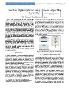
We develop in this paper the synthesis of a circular antenna array with probe feed using the FGAs discussed in the previous section. Let us consider a circular array consisting of N radiating elements distributed regularly on a circle of radius Rc, in the xOy plane as show in figure 4. Let us consider an array of N isotropic elements placed on a circular ring of radius Rc, lying on the x-y plane of an orthogonal Cartesian system O(x,y,z). The nth element of the array is located at ϕ i with the x axis, where ϕ i = 2.π .iN −1 , i=1,2,...,N.

According to the desired performances, we can consider an array comprising several rings. Among the various manners of setting out again the elements, one chose a distribution as show in Figure 5. The circle which presents the smallest ray must check the weakest spacing between the sources ( d 1 = 0.6λ ). The spacing between the circles is of d 2 = 0.6λ ( λ being the wavelength number related to the operating frequency). The total radiated field in this case is: E tot (r , θ , φ ) = E (θ , φ ).

M

N

∑∑ w i .e

(

− jk 0 . Rci . sin θ cos φ −φij

)

(14)

i =1 j =1

We use the FGAs to find the amplitude excitation

[

Fig. 4. Circular array of N elements

We consider the total radiated field Etot (r ,θ , φ ) of the array in the plane of array as the result of a sum of the contribution of each element in the observed direction. We can then write [7]: E tot (r , θ , φ ) =

N

∑ wi. i =1

=

e

− jk 0 . Ri

e − jk 0 . Ri .E (θ , φ ) Ri

(10)

N

∑ w i .e − jk .R . sin θ cos (φ −φ ) .E (θ , φ ) 0

Ri

]

vector A = A1 , A2 , ..., A N so the radiation pattern produced satisfy the desired radiation pattern specified by the pattern model as illustrated in the figure 6, we suppose that all patches have the same excitation phase(null phase). This pattern has a narrow beam with – 30dB sidelobes. The pattern is normalized to the peak value at 0 degrees and must have a 3dB beamwidth of at least 8 degrees. The –30dB sidelobe level must be met beginning at ±10 degrees and extending to ±90 degrees. The sidelobes in this case are defined relative to the peak of beam at 0 degrees. The specifications are illustrated in figure 6.

c

i

i =1

where: Ri ≅ r − Rc cos ψ i ≅ r − Rc sinθ cos(φ − ϕ i )

(11)

w i = Ai .e jα i

(12)

The radiation field of an elementary source E (θ , φ ) is computed using the two-slot model by modeling the antenna as a combination of two parallel slots of length W, width h, and spaced a distance L apart as described in [15]. The radiation from the patch is linearly polarized with the electric field directed along the patch length. We can obtain finally: e − jk0 .r E tot (r , θ , φ ) = r (13) N − j (k0 . RC . sin θ cos (φ −φi )+α i ) .∑ A i .e .E (θ , φ )

Fig. 5. Circular array with several rings.

We have choose a suitable fitness function that can guide the SGAs and FGAs optimization toward a solution that meets the desired radiation pattern as mentioned in [16]. Equations 15-17 describe the appropriate fitness function. S 1 d av = di (15) ∑ 2S + 1 i = − S

i =1

Copyright © 2007 Praise Worthy Prize S.r.l. - All rights reserved

International Review of Electrical Engineering, Vol.5 , n.2

M. Bousahla, B. Kadri, F.T. Bendimerad

Sll max =

min ( d av − d i )

(16)

∀i∈Sidelobes

fitness = d av + w1 Sll max

(17)

We have adopted a desired radiation pattern specified by a narrow beam pointed at 0 degrees as illustrated in figure 6. Figures 7 to 12 show an example of synthesis of a probe-fed circular array constituted by 96 rectangular microstrip antennas with 0.906cm width and 1.186cm long working at the frequency of 10GHz, the array is printed on a substrate with 1.1588mm height and a dielectric constant equal to 2.2. In figure 7 we present the result of circular array optimization by magnitude excitation coefficients using both SGAs and FGAs. It is clearly seen that the radiation pattern obtained by FGAs meet better the desired pattern than obtained by SGAs. The optimized amplitude excitation coefficients by both optimizer algorithms are reproduced on figure 9 and 10. The best fitness function obtained by FGAs is better than the obtained by a SGAs, this is shown in figure 8. For each generation the probabilities pc and pm are adjusted according to the response of the fuzzy controller, and shown in figures 11 and 12.

Fig. 6. Plot of the desired pattern specifications.

Where it is assumed that a number of samples of the pattern, di in dB, are taken in the beam region and the sidelobe region and that the number of samples in the beam region is equal to 2S+1. An arbitrary weight w1 is used, the goal of function (17) is to maximize the difference between d av and Sll max . First we have to find a relationship between the GAs and the array. In the case of a coded GA, each element of the array is represented by a string of bits which gives the amplitude excitation of the element; hence each element is characterized by its amplitude excitation. This relationship is shown in table 2. TABLE II. RELATIONSHIPS BETWEEN ELEMENTS OF GAS AND ARRAYS. Genetic parameters Gene Chromosome Individual Population

IV.

Antennas array Bits chain(string): Amplitude One element of array One array Several arrays

Fig. 7. Result of a circular array synthesis with 96 rectangular microstrip antennas fed by coax applying both SGAs and FGAs.

Numerical results

We have considered a circular array of radius Rc = 2λ, consisting of N=96 elements organized on six concentric rings, using the above techniques we have synthesized the pattern reproduced on figure 6. In our simulation, we have used a population size of 40 for GAs. Roulette strategy for “selection”, one–point crossover and mutation to flip bits. For the SGAs, we have used value of pc=0.75 and pm=0.03. For the FGAs, pc and pm are determined according to FLC given in section 2.1.

Copyright © 2007 Praise Worthy Prize S.r.l. - All rights reserved

Fig. 8. Comparison between fitness function obtained by the two algorithms SGAs and FGAs.

International Review of Electrical Engineering, Vol.5 , n.2

M. Bousahla, B. Kadri, F.T. Bendimerad

Fig. 12. Adjusting pm during GAs run.

Fig. 9. Optimized amplitude excitation coefficients by SGAs.

V.

Fig. 10. Optimized amplitude excitation coefficients by FGAs.

Conclusion

We have developed in this paper the synthesis of a probe-fed circular array using adaptive genetic algorithms whose control parameters are dynamically adjusted by the use of fuzzy controller. The standard genetic algorithms SGAs are subject to premature convergence problem , which is due to: control parameter not well chosen initially for a given task, parameters always being fixed even though the environment in which GA operate may be variable. The FGAs has been built for inducing exploitation/exploration relationships that avoid premature convergence problem by optimizing the parameters controlling the GAs like crossover and mutation probabilities depending on the measure of population diversity PD. The SGA converges quickly with a larger probability to get trapped in local optima, while the FGA spends more time to explore ore feasible solutions with a larger probability to find global optimal solutions. As seen in the simulation example of the circular antenna array synthesis, the performances of FGAs are much better than the SGAs in terms of: approaching better the specified desired radiation pattern and the high speed approaching of the global optimal.

References [1]

[2]

Fig. 11. Adjusting pc during GAs run.

Copyright © 2007 Praise Worthy Prize S.r.l. - All rights reserved

[3]

PRASAD, s., and CHARAN, R., On the constrained synthesis of array patterns with applications to circular and arc arrays, IEEE Trans., 1984, AP-32, (7), pp. 725-730 KARAVASSILIS, N., DAVIES, D.E.N., and GUY, c.G.: Experimental HF circular array with direction finding and null steering capabilities, IEE Proc. H, 1986, 133, (2), pp. 147-154 R. L. Haupt, An Introduction to Genetic Algorithms for Electromagnetic, IEEE Antenna and propagation Magazine, Vol. 37, pp. 7-15, 1995.

International Review of Electrical Engineering, Vol.5 , n.2

M. Bousahla, B. Kadri, F.T. Bendimerad

[4]

D. Marcano, F. Duran, Synthesis of Antenna Arrays Using Genetic Algorithms, IEEE Antenna and propagation Magazine, Vol. 42, NO. 3, June 2000. [5] D.K. Cheng, “Optimization techniques for antenna arrays”, Proc IEEE 59 (1971), 1664-1674. [6] B. Kadri, F.T. Bendimered, E. Cambiaggio, Synthèse Rigoureuse D’antennes Microrubans en Réseau non Périodique par Modélisation des Circuits d’Alimentations, 10ème Journées Internationales de Nice sur les Antennes, JINA’98, International Symposium, pp. 358-361, Nice 17-19 Novembre 1998. [7] B. Kadri, F.T. Bendimered, E. Cambiaggio, Modelisation of the Feed Network Application to Synthesis Unequally Spaced Microstrip Antennas Arrays, International Conference on Electromagnetics in Advanced Applications (ICEAA 99), pp. 371374, Torino, 13-17 September 1999. [8] D. Marcano, F. Duran, Synthesis of antenna arrays using genetic algorithms, IEEE Antennas Propagat Mag 42 (2000). [9] M. Donelli, S. Coarsi F. De Natale, M. Pastorino, A. Massa, Linear Antenna Synthesis With Hybrid Genetic Algorithm, Progress in Electromagnetics Reaseach, PIER 49, 1-22, 2004. [10] F. Herrera, M. Lozano, Adaptive Genetic Operators Based On Coevolution With Fuzzy Behaviors, IEEE Transaction on Evolutionary Computation, Vol. 5, NO. 2, April 2001. [11] K. Wang, A New Fuzzy Genetic Algorithm Based on Population Diversity, International Symposium on Computational Intelligence in Robotics and Automation, pp. 108-112, July 29 August 1, 2001, Alberta, Canada. [12] F. Herrera et M. Lozano, Adaptive genetic algorithms based on fuzzy techniques, Information Proceedings and Management of Uncertainly in Knowledge-Based Systems, pages 775–980, 1996. [13] VESCOVO, R.: Constrained and unconstrained synthesis of array factor for circular arrays, IEEE Trans., 1995, AP-43, (12), pp. 1405-1410 [14] VESCOVO, R., and CARLI, E., Null control of pattern for circular antenna arrays, Proc. 25th European Microwave Conf., 1995, 1, pp. 36 9-371 [15] R. Garg, P. Bhartia, I. Bahl, A. Ittipiboon, Microstrip Antenna design Handbook (Artech House INC, ISBN 0-89006-513-6, 2001). [16] R. L. Haupt, J. M. Johnson, Dynamic Phase-Only Array Beam Control Using a Genetic Algorithm, evolvable Hardware (EH’99), 217-224, July 19-21, Pasadena, CA, USA, IEEE Computer Society 1999.

heuristic algorithms. Fethi Tarik Bendimerad was born in Sidi BelAbbès, Algeria, in1959, he received his Phd degree from the Sophia-Antipolis University in Nice (France), in1989. He is currently a full professor at the Faculty of engineering at the Abou BekrBelkaıd University in Tlemcen, (Algeria) and the Director of the Telecommunications Laboratory. His field of interest is antenna treatment and smart antenna.

Authors’ information 1

Abou-Bakr Belkaid University, Telecommunications Laboratory, Algeria 2 Bechar University, Sciences and technologies Faculty, 08000, Bechar, Algeria Miloud Bousahla was born in Sidi BelAbbès, Algeria, in1969. He received the Magistère diplomas in 1999 from Abou BekrBelkaıd University in Tlemcen (Algeria). He is currently a Junior Lecturer in the Abou BekrBelkaıd University. Also he is a Junior Researcher within the Telecommunications Laboratory. He works on design, analysis and synthesis of antenna and conformal antenna and their applications in communication and radar systems Boufeldja Kadri was born in Bechar, Algeria, in 1972. He received the Majister degree in 1998, from the Abou Bekrbelkaid University in Tlemcen (Algeria). Since 1999, he joined the Electronic Institute in Bechar University (Algeria), where he is now an associate professor. His research interests include modeling and optimization of antenna array with

Copyright © 2007 Praise Worthy Prize S.r.l. - All rights reserved

International Review of Electrical Engineering, Vol.5 , n.2

International Journal of Electronics and Communication Engineering ISSN 0974-2166 Volume 2, Number 3 (2009), pp. 147–159 © International Research Publications House http://www.irphouse.com

Synthesis of Circular Arrays with Simulated Annealing Optimization Algorithm M. Bousahla, M. Abri, F. T. Bendimerad and N. Boukli-hacene Laboratoire de Télécommunications, Département d’Electronique Faculté des Sciences de l’Ingénieur, Université Abou-Bekr Belkaïd -Tlemcen BP 230, Pôle Chetouane, 13000 Tlemcen- Algeria

Abstract This paper presents an analysis and a synthesis of circular arrays of printed antennas. The simulated annealing technique which is a probabilistic methodology to solve combinatorial optimization problems, has been applied to optimize the amplitude of weights coefficients of the elements of the circular array in order to improve the antenna performances and to obtain a beam pattern that meet given requirements. It is seen that the optimization method is effective in designing such arrays. The power of the simulated annealing method lies in its ability to avoid the local minima and to converge to the global minimum of the cost function, thanks to the exploitation of simulated annealing potentialities and high flexibility. Key words: Printed antennas, circular arrays, analysis, synthesis, simulated annealing.

Introduction The printed antennas array aroused an interest growing during these last years, in particular in the mobiles communications fields and the monolithic structures, where the radiating elements and the phase-converters are integrated in the same substrate. They also find applications in the space techniques to ensure a specific or partial terrestrial cover, like in the military and civil field. This is mainly due to the unique feature of microstrip antennas; which are, namely, low in profile, compact in structure, light in weight, conformable to non planar surfaces, easy and inexpensive for mass production. The array association of several printed elements allows in addition an improvement of their performances, to accomplish a very particular functions, such

148

M. Bousahla, M. Abri, F. T. Bendimerad and N. Boukli-hacene

as: scanning and beam steering, jamming rejection, adaptive detection, autoadaptativity, carrying out of various radiation patterns, the directivity pattern and polarization control, …etc. The circular array, in which the radiating elements are placed on circular rings, is an array of very great practical interest. These applications are multiple: radars, sonar, terrestrial and space navigation and much of other systems [1]-[2]. In the antennas arrays domain, the synthesis problem consists in estimating the variations of the feeding weights of the radiating elements which permits to provide a radiation pattern as close as possible to a desired pattern specified by a shape pattern. The goal of this optimization is to seek for the optimal amplitude according to a precise specification. In this domain, many deterministic synthesis tools were developed. Taking into account the diversity of the goals sake by the users, one will not find a general synthesis method applicable to all cases, but rather a significant number of specific methods to each type of problem. Recently, global stochastic optimization techniques appeared, able to obtain global optima, without remaining trapped on local optima as is in the case for the deterministic methods. To achieve this goal we developed a synthesis method of these arrays by employing an optimization method based on the simulated annealing technique (SA). Simulated annealing is presented as method of finding optimal or near-optimal solutions to problems for which rigorous optimization method do not exist. The literature has reported the application of SA for general electromagnetic problems and, particularly, for the arrays synthesis [3]-[6]. This paper is organized as follows, in section II, the total radiated field of the circular array is determined and plotted in 2D and 3D. Section III presents the synthesis problem. Section IV describes the proposed method of synthesis and its basic concepts are summarized. The obtained results are reported in section V. Finally, conclusions are drawn in section VI.

Analysis A circular array consists of N radiating elements distributed regularly on a circle of radius Rc, in the xOy plane as show in Fig. 1.

Synthesis of Circular Arrays with Simulated

z

149

M

θ

r

Ri

y

ψi Rc i+1 m i

ϕi

x

Figure 1: Circular array of N elements. We consider the total radiated field Etot (r, θ, φ) as the result of a sum of the contribution of each element in the observed direction. We can then write [7]: N

E tot (r , θ , φ ) = ∑ wi i =1

e − jk0 Ri e − jk0 Ri E (θ , φ ) = Ri Ri

With: ϕ i = 2π (

i ) N

and

wi = Ai e

N

∑ wi e − jk R sinθ cos(φ −ϕ ) E (θ , φ ) 0 c

i

(1)

i =1

j αi

We can obtain finally: Etot (r ,θ ,φ ) =

e − jk0 r r

N

∑ Aie− j (k R sinθ cos(φ −ϕ )+α )E (θ ,φ ) 0 c

i

i

(2)

i =1

To fulfil the electronic sweeping function with such a device and to thus place the main lobe radiation in a direction (θ 0 , φ 0 ) , it is necessary that the term αi check the equation (3). α i = −k0 Rc sin θ 0 cos(φ0 − ϕi ) (3) The total radiated field can be written: e− jk0 r N Etot (r , θ , φ ) = Ai e jk0 Rc (sin θ cos(φ −ϕi )−sin θ 0 cos(φ0 −ϕi ))E (θ , φ ) r i =1 (4) N − jk0 r e jk 0 d 0 cos(ϕi −ζ ) = × Ai e E (θ , φ ) r i =1

∑

∑

With:

150

M. Bousahla, M. Abri, F. T. Bendimerad and N. Boukli-hacene

⎧ sin θ sin φ − sin θ0 sin φ0 ⎫ ⎬ ⎩ sin θ cos φ − sin θ0 cos φ0 ⎭

ζ = arctg ⎨

(5)

and

[

]

1

d 0 = Rc (sin θ cos φ − sin θ 0 cos φ0 )2 + (sin θ sin φ − sin θ 0 sin φ0 )2 2 (6) According to the desired performances, we can consider an array comprising several crowns. Among the various manners of setting out again the elements, one chose a distribution as show in Fig. 2.

Y Z

Rc3

Rc1

Rc4

Rc2 X

Figure 2: Circular array with several crowns.

The circle which presents the smallest ray must check the weakest spacing between the sources (d1= 0.6λ). The spacing between the circles is of d2= 0.6λ (λ being the wavelength number related to the operating frequency). The total radiated field in this case is: M

Etot (r ,θ ,φ ) = E (θ ,φ )∑

N

∑ wij e

i =1 j =1

(

− jk 0 Rci sin θ cos φ −ϕ ij

)

(7)

Synthesis of Circular Arrays with Simulated

151

Synthesis problem The synthesis problem in which one is interested consists in minimizing the levels of the harmful side lobes to the useful radiation [7]-[10]. (8) Wi = Ai e − jϕ i Where: Wi are complex weights to each element. Ai is the amplitude of the excitation and φi is the phase of the excitation. The synthesis consists of minimizing a criterion of variation δ between the synthesized pattern Fs(θ,φ) and the desired pattern Fd(θ) defined by a shape pattern imposed in advance by the user. The optimization problem then consists in minimizing the quadratic error. δ (θ , ϕ ) = ∑ Fs (θ , ϕ ) − Fd (θ )

2

(9)

θ

Where : Fd is the desired function and Fs is the synthesized function. The SA described in next section, has been found to be very effective for the optimization of the array, thanks to its robustness and inherent ability to accommodate a variety of constraints.

Basic concepts of simulated annealing SA is a probabilistic method based on concepts deriving from statistical mechanics by the means of the famous method of annealing used by the metallurgists. This method uses the Metropolis algorithm [11]. This algorithm is precisely used to randomly draw a continuation from microscopic configurations by respecting the proportions of Boltzmann relating to balance at a given temperature. As for the algorithm of iterative improvement, the algorithm of Metropolis makes it possible to explore by a random walk a graph whose tops are the microscopic configurations of the system. In the case of the iterative improvement, displacement in the graph is always carried out towards the configurations of decreasing cost, while the algorithm of Metropolis allows sometimes transitions towards configurations from higher cost. In optimization, an iterative research which accepts only the new points corresponding to a lower value of the function is equivalent to a physical system which reaches temperature equal to zero quickly, which brings us at local minima. On the other hand simulated annealing seeks to converge towards the global minimum thanks to the control of the parameter temperature. The algorithm of Metropolis calculates the new function E new = f ( x1 ) , with x1 the new point generated starting from a function g (Δx) where Δx is the difference between the new point and the current point. The majority of the optimization methods using simulated annealing choose their new point with variable distances from their starting point or running. If the solution obtained is better than the preceding one, then this solution is accepted. If the

152

M. Bousahla, M. Abri, F. T. Bendimerad and N. Boukli-hacene

preceding solution remains better, a law of probability of acceptance intervenes in order to decide to keep or reject this value. Probability of acceptance determined by a function H, depends on the temperature T and difference between the two values of the function. As an example, while referring to the Boltzmann law, definite as follows [12]: 1 ≈ exp(− ΔE ) (10) H= T 1 + exp(ΔE ) T Where E = f ( x) represent the system energy, and ΔE = E new − E represent the difference in energy between the new point and the preceding point. In order to accept or to reject a point for which Enew is not better than E, one carries out the lots of a random variable P on [0, 1]. If the variable obtained is lower than H the point is then accepted. In the contrary case, the new point is refused. When a new point is accepted, even if the corresponding value of the function is worse than with the preceding point, it becomes then the new point running or solution. At the beginning, the temperature T must be large and a new point must be roughly accepted once on two. With the progression of the algorithm in time, the temperature T is reduced, implying a fall of the acceptance probability of the points. In fact, the value called ‘‘temperature’’ T is only one parameter making it possible to control the amplitude of the movements and makes it possible to avoid the minima. When the temperature is null, the probability of transition becomes unit. If energy decreases at the time of the transformation, and that it is null in the opposite case: the algorithm of Metropolis is then identical to an algorithm of iterative improvement, in this case, one is likely to finish trapped in local minima. On the other hand, when the temperature is not null, the algorithm can choose points with a value of the higher function, which makes it possible to avoid the minima in favour of global minima good located in the workspace. Simulated annealing algorithms are expected to arrive at a good solution only in a statistical sense as in principale an infinitely large number of iterations are necessary to attain the global minimum. In practice to be useful, an acceptable solution must be attained in a finite reasonable number of iterations. For this to be possible, the cooling schedule must be carefully chosen so that the temperature falls only as fast as is compatible with maintaining a quasi equilibrium, otherwise the algorithm will lock in a secondary minimum. Various cooling schedules have been experimented with (step by step, linear, geometric and exponential) and, as expected, it is important to cool slowly, particularly at low temperatures. Finally, for the tests described here, the modified exponential cooling schedule recommended by Rees Ball [13] is adopted. However, if a modified exponential scheduling is chosen, almost all process running give slightly different results in term of energy and weight values. This means that the resulting configuration is stable and close to the optimal one. We used for the synthesis of our radiation pattern the simulated annealing algorithm presented by Corona [14]. This algorithm was tested by various authors and was compared with other techniques like the simplex or gradient conjugate known of

Synthesis of Circular Arrays with Simulated

153

the functions comprising local minima. It proved that it always found the global minima which are not the case of the other methods. The algorithm is very simple and is presented in the following general form as shown in Fig. 3.

Initialize the values X0; v0; T0; Ns; Nt; ε ; i=j=k=m=0 ; h=1 Xopt =X0 ; fopt = f0 ; nh = 0 ; f0 = f(X0)

X’ = Xi + r. vm,h .eh With r∈[-1,1]

No

( r + 1) 2

h = h+1

x ' h = a h + ( bh − a h ).

ah ≤ xh ≤ bh

Yes

h = h+1

Calculation f’ = f(X’) No

h = h+1

f’ ≤ fi ?

Yes

Using the function H (Probability of acceptance) In case of acceptance, one has then Xi+1 =X’ , fi+1 = f’ Increment i and nh

Xi+1 =X’ , fi+1 = f’ Incrémenter i et nh Xopt = X’ , fopt = f’

Yes

h≤N? No

H=1 and j=j+1

M. Bousahla, M. Abri, F. T. Bendimerad and N. Boukli-hacene

154

Yes

j ≤ Ns ?

Update of the vectors vm,h for each nh ⎡ ⎤ Ns − 0.6 ⎥ ⎢ Vm +1, h = Vm, h ⎢1 + ch if nh > 0.6 Ns ⎥ 0 .4 ⎢ ⎥ ⎣ ⎦ Vm, h if nh < 0.4 Ns Vm +1, h = 0.4 − nh ⎤ ⎡ Ns ⎥ ⎢ ⎥ ⎢1 + ch 0 .4 ⎥ ⎢ ⎦ ⎣ Vm +1, h = Vm, h

otherwise

j = 0 ; n K= 0 Increment ‘m’ Yes

m ≤ NT ? No Tk+1 = rt . Tk K = k+1 ; m = 0 f k = fi *

Increment i Xi = Xopt fi = fopt Stop criterion End

f k * − f opt < ε

yes

f k* − f K −u < ε

No

u=1…Ns.

fopt