Circuit Switching Computer Networks

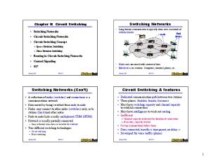
Network resources (e.g., bandwidth) divided into “pieces” Pieces allocated to and reserved for calls Resource idle if not used by owner (no sharing) Ways to divide link bandwidth into “pieces” •  frequency division multiplexing (FDM) frequency

Lecture 36: QoS, Priority Queueing, VC, WFQ

Example: 4 users time

•  time division multiplexing (TDM) frequency

time

Packet Switching Each end-to-end data stream divided into packets

Bandwidth division into “pieces” Dedicated allocation Resource reservation

Packets from multiple users share network resources Each packet uses full link bandwidth Resources used as needed Resource contention: •  aggregate resource demand can exceed amount available •  congestion: packets queued, wait for link use •  store and forward: packets move one hop at a time •  each node receives complete packet before forwarding

Packet Switching: Statistical Multiplexing 10 Mbps Ethernet

A B

statistical multiplexing

C

1.5 Mbps queue of packets waiting for output link

D

E

Sequence of A’s and B’s packets does not have a fixed pattern statistical multiplexing

Pros and Cons of Packet Switching

Packet vs. Circuit Switching Packet switching allows more users to use network! For example: •  1 Mbps link •  each user: •  sends 100 kbps when “active” •  active 10% of time

N users

1 Mbps link

circuit-switching: 10 users packet switching: with 35 users, probability that more than 10 are active at the same time < .0004

Advantages: great for bursty data

•  resource sharing •  simpler, no call setup

Disadvantages: excessive congestion, packet delay and loss •  protocols needed for reliable data transfer •  congestion control •  no service guarantee: “best-effort” service

Better than Best-Effort Service

Example: HTTP vs. VoIP Traffic

Approach: deploy enough link capacity such that congestion doesn’t occur, traffic flows without queueing delay or overflow buffer loss

1Mbps VoIP shares 1.5 Mbps link with HTTP •  HTTP bursts can congest router, cause audio loss •  want to give priority to audio over HTTP

•  advantage: low complexity in network mechanisms

•  packets can be differentiated by port number or

•  disadvantage: high bandwidth costs, most of the time

•  packets can be marked as belonging to different classes



bandwidth is under utilized (e.g., 2% average utilization)

Alternative: multiple classes of service

1 Mbps phone

R1

R2

•  partition traffic into classes (not individual connections) •  network treats different classes of traffic differently

1.5 Mbps link

Priority Queueing

Traffic Metering/Policing

Send highest priority queued packet first

high priority queue arrivals

• multiple classes, with different priorities classifier •  fairness: gives priority to low priority queue some connections 2 •  delay bound: higher priority 4 1 3 connections have lower delay arrivals •  but within the same priority, packet in service 1 3 2 4 still operates as FIFO, hence delay not bounded departures 1 3 2 4 •  relatively cheap to operate (O(log N)), N number of packets in queue

departures

What if applications misbehave (VoIP sends higher than declared rate)? Marking and/or policing:

server

•  force sources to adhere to bandwidth allocations •  provide protection (isolation) for one class from others •  done at network ingress

5

1 Mbps phone

5

5

R1

R2 1.5 Mbps link

packet marking and/or policing

Policing Mechanisms Goal: limit traffic to not exceed declared parameters Three commonly used criteria: 1. average rate: how many packets can be sent per averaging time interval •  crucial question: what is the averaging interval length? •  100 packets per sec or 6,000 packets per min have the same average!

2. peak rate: packet sent at link speed, inter-packet gap is transmission delay •  e.g., 6,000 packets per min (ppm) avg.; 1,500 ppsec peak

3. (max.) burst size: maximum number of packets allowed to be sent at peak rate without intervening idle period

Token-Bucket Filter Limit packet stream to specified burst size and average rate

• bucket can hold at most b tokens • new tokens generated at the rate of r tokens/sec • new tokens dropped once bucket is full • packet can be sent only if there’s enough tokens in buffer to cover it • assuming 1 token is needed per packet, over interval of length t: number of packets metered out is ≤ (rt + b)

Circuit vs. Packet Switching Packet switching: data sent through the network in discrete “chunks” Circuit switching: dedicated circuit per call • end-to-end resources reserved for calls •  link bandwidth, switch capacity •  call setup required

• dedicated resources: no sharing •  guaranteed performance •  resource idle if not used by owner

Pros and Cons of Packet Switching Advantages: great for bursty data

•  resource sharing •  simpler, no call setup

Disadvantages: excessive congestion, packet delay and loss •  protocols needed for reliable data transfer •  congestion control •  no service guarantee of any kind

How to provide circuit-like quality of service? •  bandwidth and delay guarantees needed for

multimedia apps

Packet-Switched Networks No call setup at network layer No state to support end-to-end connections at routers •  no network-level concept of “connection” •  route may change during session

Packets forwarded using destination host address •  packets between same source-destination pair may take

different paths

application transport network 1. send data data link physical

application transport 2. receive data network data link physical

Virtual Circuits (VC) Datagram network provides network-layer connectionless service VC network provides network-layer connectionoriented service Analogous to the transport-layer services, but: •  service is host-to-host, as opposed to socket-to-socket •  implementation in network core

Source-to-destination path behaves much like a telephone circuit •  in terms of performance, and •  network actions along the path

Virtual Circuits

Virtual Circuits

A VC comprises:

Signalling protocol:

1.  path from source to destination

•  used to setup, maintain, teardown VC

•  each call must be set up before data can flow

•  e.g., ReSource reserVation Protocol (RSVP)

•  requires signalling protocol

•  fixed path determined at call setup time,

remains fixed throughout call

•  every router on path maintains state

application transport 5. data flow begins network 4. call connected data link physical

for each passing connection/flow

•  link, router resources (bandwidth, buffers)

may be allocated to VC

2.  VC numbers, one number for each link along path •  each packet carries a VC identifier (not destination host address)

1. initiate call

6. receive data 3. accept call

application transport network data link physical

2. incoming call

3.  entries in forwarding tables in routers along path

VC Forwarding Table

Per-VC Resource Isolation

Packet belonging to a VC carries a VC number

To provide circuit-like quality of service

VC number must be changed for each link

•  resources allocated to a VC must be isolated from other

traffic

New VC number obtained from forwarding table

Bit-by-bit Round Robin:

Examples: MPLS, Frame-relay, ATM, PPP Forwarding table on router NW:

VC number NW

12

1

interface number

3

22

2

32

incoming interface

incoming VC#

outgoing interface

outgoing VC#

1

12

2

22

2

63

1

18

3

7

2

17

1

97

3

87

…

…

…

…

Routers maintain connection state information!

•  cyclically scan per-VC queues, sending one bit from each VC (if present) •  1 round, R( ), is defined as all non-empty queues have been served 1 quantum •  R(t5) = 2 •  time at Round 3? Round 4?

t9 t6 t3 t0

4321 t7 t4 t1

321 t11 t10 t8 t5 t2

5 4321

A.k.a. Generalized Processor Sharing (GPS)

1 bit

RR

µ

Packetized Scheduling

Fluid-Flow Approximation

Packet-by-packet Round Robin:

A continuous service model

• cyclically scan per-flow queues, sending one t5 t4 t2 t1 packet from each flow (if present) 2 1 • Problem: gives bigger share to t9 t8 t7 t6 t3 flows with big packets

• instead of thinking of each quantum as serving discrete bits in a given order • think of each connection as a fluid stream, described by the speed and volume of flow

65 4321

Packet-by-packet Fair Queueing:

At each quantum the same amount of fluid from each (non-empty) stream flows out concurrently

µ

RR

• compute F: finish round, the round a packet finishes service • simulates fluid-flow RR in the computation of F’s • serve packets with the smallest F first

RR

µ

t8 t7 t3 t2

2 F=4

1 F=2

µ

t9 t6 t5 t4 t1

FQ

65 4321 F=1 F=5 F=3 F=2 F=4 F=6

R5 R4 R3 R2 R1

Round# vs. Wall-Clock Time

Start and Finish Rounds

Let:

When does packet i finish service? t8 t7 t3 t2 F αi = S αi + P αi, α 2 1 where P i is the service time (in t9 t6 t5 t4 t1 rounds) of packet i and S αi the 65 4321 service start round At what round does packet i of flow α start seeing service? S αi = MAX(F αi–1, Aαi) F=4

α i

• S αi = F αi–1 if there is a queue, Aαi otherwise • Aαi = R(t αi): round at the time packet i arrives

a

c

b

tαi +δa

tαi +δ2

α i

F=2

F=1 F=5 F=3 F=2 F=4 F=6

Round#

• time: wall-clock time F • round: virtual-clock time • µ = 1 unit P • t αi: arrival time of packet i of flow α • Nac(t): #active flows at time t S

µ FQ

α i

Computing the rate of change:

t a: Nac = 1, ∂R/∂t = µ/Nac(t) = 1, b: Nac = 2, ∂R/∂t = ½, δ2 = 2∗δ1 c: at the beginning, Nac = 1, ∂R/∂t = 1, halfway serving packet i, a packet belonging to another flow arrives, Nac = 2, ∂R/∂t = ½ α i

tαi +δ1

Wall-clock time

As Nac(t) changes, finish round stays the same, actual time stretches

Arrival Round Computation

Round Computation Example Scenario:

When packet i of an active flow arrives, its finish round is α α α α computed as F i = F i–1 + P i , where F i–1 is the finish round of the last packet in α’s queue

• flows A has 1 packet of size 1 arriving at time t0 • flows B and C each has 1 packet of size 2 arriving at time t0 • flow A has another packet of size 2 arriving at time t4

Slope (∂R/∂t): a = ⅓, b = ½, c = ⅓, d = 1

If flow α is inactive, there’s no packet in its queue, F αi = Aαi + P αi , how do we compute Aαi?

Round# 3.5

2 1.5

What is the arrival 1 nd round of A’s 2 packet? 0 R(t A2) = 1.5

FA2

d

FB1 FC1

S A2 = A A2

c

FA1

b a 3

4

5.5 7 Wall-clock time

If flow α has been inactive for Δt time and there has been Nac flows during the whole time, we can perform round catch up: Aαi = F αi–1 + Δt(1/Nac) Iterated deletion: if Nac has changed, one or more times, over Δt, round catch up must be computed in piecewise fashion, every time Nac changes expensive

assuming fluid-flow approximation

Weighted Fair Queueing

(Weighted) Fair Queueing

Weighted-Fair Queueing (WFQ):

Credit accumulation:

• generalized Round Robin • each VC/flow/class gets weighted amount of service in each cycle • P αi = Lαi/(ωµ), Lαi size of packet

•  allows a flow to have a bigger share if it has been idle •  discouraged because it can be abused: accumulate

credits for a long time, then send a big burst of data

Characteristics of (W)FQ:

t5 t4 t3 t2

2 F=2

1

ω=⅔ ω=2

F=1

t9 t8 t7 t6 t1

65 4321 F=5 F=3 F=1 F=6 F=4 F=2

WFQ ω=1 ω=⅓

µ

•  max-min fair •  bounded delay •  expensive to implement

Max-Min Fair

Max-Min Fair

In words: max-min fair share maximizes minimum share of flows whose demands have not been fully satisfied 1. no flow gets more than its request 2. no other allocation satisfying condition 1 has a higher minimum allocation 3. condition 2 remains true as we remove the flow with minimal request

Let: µtotal: total resource (e.g., bandwidth) available µi: total resource given to (flow) i µfair: fair share of resource ρi: request for resource by (flow) i Max-Min fair share is µi = MIN(ρi, µfair) µtotal = ∑ µi, i = 1 to n

Max-Min Fair Share Example Let: µtotal = 30

i

ρi

µi

A

12

11

B

11

11

C 8 8 Initialy µfair = 10 ρC = 8, so unused resource (10 – 8 = 2) is divided evenly between flows whose demands have not been fully met Thus, µfair for A and B = 10 + 2/2 = 11

Providing Delay Guarantee Token bucket filter and WFQ combined provides guaranteed upper bound on delay arriving traffic arriving traffic

token rate, r bucket size, b

WFQ

per-flow rate, μf

Dmax = b/μf QoS guarantee!

Same inefficiency issue as with circuit switching: allocating nonsharable bandwidth to flow leads to low utilization if flows don’t use their allocations

Limitations of (W)FQ

Work Conservation

t8 t7 t3 t2

2

1

Round computation expensive: t9 t6 t5 t4 t1 FQ must re-compute R every time 65 4321 number of active flows changes Unless packet transmission can be pre-empted, fairness is “quantized” by minimum packet size F=4

F=2

F=1 F=5 F=3 F=2 F=4 F=6

• once a big packet starts transmission, newly arriving packets with smaller finish times must wait for completion of transmission • flows with relatively smaller packets will suffer this more than flows with larger packets

µ

Work-conserving schedulers: •  doesn't go idle whenever there is packet in queue •  makes traffic burstier •  could require more buffer space downstream



Non-work conserving schedulers: •  only serve packets whose service times have arrived •  more work to determine whether packets' service times

have arrived •  smooth out traffic by idling link and pacing out packets