5/29/2014
Chapter 5 Models for Uncertain Demand
Introduction • In this chapter, we introduce uncertainty and develop some models where variables are not known exactly, but follow known probability distributions. • In particular, we focus on variable demand. • Many models have been developed in this area, so we will concentrate on the most widely used.
1
5/29/2014
Uncertainty in Stocks • In practice, there is almost always some uncertainty in stocks – – – – – – – –
As prices rise with inflation, operations change, new products become available, supply chains are disrupted, competition alters, new laws are introduced, the economy varies, customers and suppliers move, and so on.
• From an organization’s point of view, the main uncertainty is likely to be in customer demand, which might appear to fluctuate randomly or follow some long-term trend.
Uncertainty in Stocks • Unknown – in which case we have complete ignorance of the situation and any analysis is difficult; • Known (and either constant or variable) – in which case we know the values taken by parameters and can use deterministic models; • Uncertain – in which case we have probability distributions for the variables and can use probabilistic or stochastic models.
2
5/29/2014
Uncertainty in Stocks: Areas with Uncertainty • Demand. Aggregate demand for an item usually comes from a number of separate customers. The organization has little real control over who buys their products, or how many they buy. Random fluctuations in the number and size of orders give a variable and uncertain overall demand. • Costs. Most costs tend to drift upwards with inflation, and we cannot predict the size and timing of increases. On top of this underlying trend, are short-term variations caused by changes to operations, products, suppliers, competitors, and so on. Another point is that changing the accounting conventions can change the apparent costs.
Uncertainty in Stocks: Areas with Uncertainty • Lead time. There can be many stages between the decision to buy an item and actually having it available for use. Some variability in this chain is inevitable, especially if the item has to be made and shipped over long distances. A hurricane in the Atlantic, or earthquake in southern Asia can have surprisingly far-reaching effects on trade. • Deliveries. Orders are placed for a certain number of units of a specified item, but there are times when these are not actually delivered. The most obvious problem is a simple mistake in identifying an item or sending the right number. Other problems include quality checks that reject some delivered units, and damage or loss during shipping. On the other hand, a supplier might allow some overage and send more units than requested. The deliveries ultimately depend on supplier reliability.
3
5/29/2014
Uncertainty in Stocks: Areas with Uncertainty • Overall, the key issue for probabilistic models is the lead time demand. • It does not really matter what variations there are outside the lead time, as we can allow for them by adjusting the timing and size of the next order. • Our overall conclusion is that uncertainty in demand and lead time is particularly important for inventory management.
Uncertain Demand • Even when the demand varies, we could still use the mean value in a deterministic model. • We know that costs rise slowly around the economic order quantity, so this should give a reasonable ordering policy. • In practice, this is often true – but we have to be careful as the mean value can give very poor results.
4
5/29/2014
Worked Example 1: Uncertain Demand Demand for an item over the past 6 months has been 10, 80, 240, 130, 100 and 40 units respectively. The reorder cost is £50 and holding cost is £1 a unit a month, and any orders placed in one month become available in the following month. How good is an ordering policy based on average values?
Worked Example 1: Uncertain Demand Given: Average D = 100 units/mo. RC = £50 an order HC = £1 per unit-mo. LT = 1 mo. Mo. Opening stock Delivery Demand Closing stock
1 0 100 10 90
2 90 100 80 110
Calculated with EOQ model: Qo = 100 units To = 1 mo. ROL = LT × D = 100 units 3 110 0 240 -130
4 0 100 130 -30
5 0 100 100 0
6 0 100 40 60
Assumptions: • an opening stock of 0, but an order of 100 units arriving at the start of month 1; • orders are placed every month when the closing stock is below 100 units, and the delivery is available to meet demand in the following month; • all unmet demand (i.e. negative closing stock) is lost.
5
5/29/2014
Worked Example 1: Uncertain Demand 250
200
Stock level
150
100
50
0 0
1
2
3
4
5
6
7
-50
-100
-150
Uncertain Demand • Assume that the overall demand for an item is made up of small demands from a large number of customers, then we can reasonably say that the overall demand is Normally distributed. • A deterministic model will use the mean of this distribution and then calculate the reorder level as: Reorder Level = Mean Demand × Mean Lead Time • The actual lead time demand is likely to be either above or below the expected value. The problem is that a Normal distribution gives a demand that is higher than expected in 50% of stock cycles – so we can expect shortages and unsatisfied customers in half the cycles.
6
5/29/2014
Uncertain Demand
Ideal case
Models for Discrete Demand: Marginal Analysis • The models we have looked at so far consider stable conditions where we want the minimal cost over the long term. • Sometimes, however, we need models for the shorter term and, in the extreme, for a single period. (a newsagent buys a Sunday magazine from its wholesaler.) • We can tackle this problem of ordering for a single cycle by using a marginal analysis, which considers the expected profit and loss on each unit. • If the demand is discrete, and we place a very small order for Q units, the probability of selling the Qth unit is high and the expected profit is greater than the expected loss. • If we place a very large order, the probability of selling the Qth unit is low and the expected profit is less than the expected loss.
7
5/29/2014
Models for Discrete Demand: Marginal Analysis • Based on this observation, we might suggest that the best order size is the largest quantity that gives a net expected profit on the Qth unit – and, therefore, a net expected loss on the (Q+1)th and all following units. • Ordering less than this value of Q will lose some potential profit, while ordering more will incur net costs.
Models for Discrete Demand: Marginal Analysis Assume that: • We buy a number of units, Q; • Some of these are sold in the cycle to meet demand, D; • Any units left unsold, Q−D, at the end of the cycle are scrapped at a lower value; • Prob(D>Q) = probability demand in the cycle is greater than Q; • SP= selling price of a unit during the cycle; • SV= scrap value of an unsold unit at the end of the cycle. • The profit on each unit sold is (SP − UC), so the expected profit on the Qth unit = Prob(D≥Q) × (SP−UC) • And the loss on each unit scrapped is (UC − SV), so the expected loss = Prob(D< Q) × (UC−SV).
8
5/29/2014
Models for Discrete Demand: Marginal Analysis • We will only buy Q units if the expected profit is greater than the expected loss and: 𝑃𝑟𝑜𝑏(𝐷 ≥ 𝑄) × (𝑆𝑃 − 𝑈𝐶) ≥ 𝑃𝑟𝑜𝑏(𝐷 < 𝑄) × (𝑈𝐶 − 𝑆𝑉) ≥ (1 − 𝑃𝑟𝑜𝑏(𝐷 ≥ 𝑄)) × (𝑈𝐶 − 𝑆𝑉) • We can rearrange to give the general rule, that we place an order for the largest value of Q which still has: 𝑈𝐶 − 𝑆𝑉 𝑃𝑟𝑜𝑏(𝐷 ≥ 𝑄) ≥ 𝑆𝑃 − 𝑆𝑉 • Starting with a small value of Q, we can iteratively increase it, and the expected profit continues to rise while the inequality remains valid. • At some point the inequality becomes invalid, showing the last units would have an expected loss, and net profit begins to fall. • This identifies the best value for the order size.
Worked Example 2: Marginal Analysis Warehouse Accessories Inc. are about to place an order for industrial heaters for a forecast spell of cold weather. They pay $1,000 for each heater, and during the cold spell sell them for $2,000 each. Demand for the heaters declines markedly after a cold spell, and any unsold units are discounted to $500. Previous experience suggests the likely demand for heaters is as follows. Demand Probability
1
2
3
4
5
0.2
0.3
0.3
0.1
0.1
How many heaters should the company buy?
9
5/29/2014
Worked Example 2: Marginal Analysis UC= 1000 SP= 2000 SV= 500 (UC-SV)/(SP-SV)= 0.3333 Q Prob(D>=Q)
1 1 Valid
2 0.8 Valid Demand 1 2 3 4 5 Expected
3 0.5 Valid Q=1 1000 1000 1000 1000 1000 1000
4 0.2 Inv.
5 0.1
Q=2 500 2000 2000 2000 2000 1700
Q=3 0 1500 3000 3000 3000 1950
Q=4 -500 1000 2500 4000 4000 1750
Q=5 -1000 500 2000 3500 5000 1400
Prob 0.2 0.3 0.3 0.1 0.1
Models for Discrete Demand: Newsboy Problem • This marginal analysis is particularly useful for seasonal goods. • A standard example is a newsboy selling papers on a street corner. The newsboy has to decide how many papers to buy from his supplier when customer demand is uncertain. If he buys too many papers, he is left with unsold stock which has no value at the end of the day; if he buys too few papers he has unsatisfied demand which could have given a higher profit. • Because of this illustration, single period problems are often called newsboy problems. • The marginal analysis described above is based on intuitive reasoning, but we can use a more formal approach to confirm the results.
10
5/29/2014
Models for Discrete Demand: Newsboy Problem • Assuming the newsboy buys Q papers, and then: • If demand, D, is greater than Q the newsboy sells all his papers and makes a profit of Q × (SP − UC) (assuming there is no penalty for lost sales); • If demand, D, is less than Q, the newsboy only sells D papers at full price, and gets the scrap value, SV, for each of the remaining Q− D. Then his profit is D × SP + (Q− D)× SV − Q× UC. • The optimal value for Q maximizes this expected profit.
Models for Discrete Demand: Newsboy Problem D
Revenue
Cost
Profit
Prob.
0
0×SP+(Q-0)×SV
Q×UC
0×SP+(Q-0)×SV-Q×UC
Prob(0)
1
1×SP+(Q-1)×SV
Q×UC
1×SP+(Q-1)×SV-Q×UC
Prob(1)
⋮
⋮
⋮
⋮
⋮
Q-1
(Q-1)×SP+1×SV
Q×UC
(Q-1)×SP+1×SV-Q×UC
Prob(Q-1)
Q
Q×SP+0×SV=Q×SP
Q×UC
Q×SP+0×SV-Q×UC=Q(SP-UC)
Prob(Q)
Q+1
Q×SP+0×SV=Q×SP
Q×UC
Q×SP+0×SV-Q×UC=Q(SP-UC)
Prob(Q+1)
⋮
⋮
⋮
⋮
⋮
∞
Q×SP+0×SV=Q×SP
Q×UC
Q×SP+0×SV-Q×UC=Q(SP-UC)
Prob(∞)
11
5/29/2014
Models for Discrete Demand: Newsboy Problem • The total expected profit from buying Q newspapers, EP(Q), is the sum of the profits multiplied by their probabilities. ∞
𝐸𝑃 𝑄 =
𝑃𝑟𝑜𝑓𝑖𝑡𝐷 × 𝑃𝑟𝑜𝑏(𝐷) 𝐷=0
𝑄
=
∞
[𝐷 × 𝑆𝑃 + 𝑄 − 𝐷 × 𝑆𝑉 − 𝑄 × 𝑈𝐶] × 𝑃𝑟𝑜𝑏 𝐷 + 𝐷=0 𝑄
∞
= 𝑆𝑃 ×
𝐷 × 𝑃𝑟𝑜𝑏 𝐷 + 𝑄 × 𝐷=0
𝑄 𝑆𝑃 − 𝑈𝐶 𝑃𝑟𝑜𝑏(𝐷) 𝐷=𝑄+1 𝑄
𝑃𝑟𝑜𝑏(𝐷) + 𝑆𝑉 × 𝐷=𝑄+1
(𝑄 − 𝐷) × 𝑃𝑟𝑜𝑏(𝐷) − 𝑄 × 𝑈𝐶 𝐷=0
𝐸𝑃 𝑄 − 1 𝑄−1
= 𝑆𝑃 ×
∞
𝑄−1
𝐷 × 𝑃𝑟𝑜𝑏 𝐷 + (𝑄 − 1) × 𝐷=0
𝑃𝑟𝑜𝑏(𝐷) + 𝑆𝑉 × 𝐷=𝑄
(𝑄 − 1 − 𝐷) × 𝑃𝑟𝑜𝑏(𝐷) − (𝑄 − 1) × 𝑈𝐶 𝐷=0
∞
𝐸𝑃 𝑄 − 𝐸𝑃 𝑄 − 1 = 𝑆𝑃 ×
𝑄−1
𝑃𝑟𝑜𝑏 𝐷 + 𝑆𝑉 × 𝐷=𝑄
𝑃𝑟𝑜𝑏 𝐷 − 𝑈𝐶 𝐷=0
Models for Discrete Demand: Newsboy Problem ∞
𝐸𝑃 𝑄 − 𝐸𝑃 𝑄 − 1 = 𝑆𝑃 ×
𝑄−1
𝑃𝑟𝑜𝑏 𝐷 + 𝑆𝑉 × 𝐷=𝑄
𝑃𝑟𝑜𝑏 𝐷 − 𝑈𝐶 𝐷=0
∞
𝐸𝑃 𝑄 − 𝐸𝑃 𝑄 − 1 = 𝑆𝑃 ×
∞
𝑃𝑟𝑜𝑏 𝐷 + 𝑆𝑉 × [1 − 𝐷=𝑄
∞
𝐸𝑃 𝑄 − 𝐸𝑃 𝑄 − 1 = 𝑆𝑃 − 𝑆𝑉 ×
𝑃𝑟𝑜𝑏 𝐷 ] − 𝑈𝐶 𝐷=𝑄
𝑃𝑟𝑜𝑏 𝐷 − (𝑈𝐶 − 𝑆𝑉) 𝐷=𝑄 ∞
𝐸𝑃 𝑄 + 1 − 𝐸𝑃 𝑄 = 𝑆𝑃 − 𝑆𝑉 ×
𝑃𝑟𝑜𝑏 𝐷 − (𝑈𝐶 − 𝑆𝑉) 𝐷=𝑄+1
The optimal Q is 𝑄𝑜 , so that 𝐸𝑃 𝑄𝑜 − 𝐸𝑃 𝑄𝑜 − 1 > 0 > 𝐸𝑃 𝑄𝑜 + 1 − 𝐸𝑃 𝑄𝑜
𝑷𝒓𝒐𝒃 𝑫 ≥ 𝑸𝒐 >
𝑼𝑪 − 𝑺𝑽 > 𝑷𝒓𝒐𝒃(𝑫 ≥ 𝑸𝒐 + 𝟏) 𝑺𝑷 − 𝑺𝑽
12
5/29/2014
Models for Discrete Demand: Newsboy Problem
Worked Example 3: Marginal Analysis In recent years the demand for a seasonal product has had the following pattern. Demand Probability
1
2
3
4
5
6
7
8
0.05
0.1
0.15
0.2
0.2
0.15
0.1
0.05
It costs £80 to buy each unit and the selling price is £120. How many units would you buy for the season? What is the expected profit? Would your decision change if the product has a scrap value of £20?
13
5/29/2014
Worked Example 3: Marginal Analysis Demand Probability
1 0.05
UC= SP= SV= (UC-SV)/(SP-SV)= Q Prob(D>=Q)
2 0.1
3 0.15
4 0.2
5 0.2
6 0.15
7 0.1
8 0.05
2 0.95 Valid
3 0.85 Valid
4 0.7 Valid
5 0.5 Inv.
6 0.3
7 0.15
8 0.05
80 120 0 0.6667 1 1 Valid
Worked Example 3: Marginal Analysis Demand 1 2 3 4 5 6 7 8 Expected
Q=1 40 40 40 40 40 40 40 40 40
Q=2 -40 80 80 80 80 80 80 80 74
Q=3 -120 0 120 120 120 120 120 120 96
Q=4 -200 -80 40 160 160 160 160 160 100
Q=5 -280 -160 -40 80 200 200 200 200 80
Q=6 -360 -240 -120 0 120 240 240 240 36
Q=7 -440 -320 -200 -80 40 160 280 280 -26
Q=8 -520 -400 -280 -160 -40 80 200 320 -100
Prob 0.05 0.1 0.15 0.2 0.2 0.15 0.1 0.05
14
5/29/2014
Worked Example 4: Marginal Analysis Zennor Package Holiday Company is about to block book hotel rooms for the coming season. The number of holidays actually booked is equally likely to be any number between 0 and 99 (for simplicity rather than reality). Each room booked costs Zennor €500 and they can sell them for €700. How many rooms should the company book if unsold rooms have no value? How many rooms should it book if unsold rooms can be sold as last-minute bookings for €200 each?
Worked Example 4: Marginal Analysis UC=
500
SP=
700
SV= (UC-SV)/(SP-SV)=
0 0.7143
UC=
500
SP=
700
SV=
200
(UC-SV)/(SP-SV)=
0.6
𝑄𝑜 = 29
𝑄𝑜 = 40
15
5/29/2014
Models for Discrete Demand: Discrete Demand with Shortages • We can extend the newsboy problem by looking at models for discrete demand over several periods. • A useful approach to this incorporates the scrap value into a general shortage cost, SC, which includes all costs incurred when customer demand is not met. • We can illustrate this kind of analysis by a model that has: – discrete demand for an item which follows a known probability distribution; – relatively small demands and low stock levels; – a policy of replacing a unit of the item every time one is used; – the objective of finding the optimal number of units to stock. – e.g., situation with stocks of spare parts for equipment.
Models for Discrete Demand: Discrete Demand with Shortages • The objective is to find an optimal stock level rather than calculate an optimal order quantity. • When an amount of stock, A, is greater than the demand, D, there is a cost for holding units that are not used. This is (A − D) × HC per unit of time. • When demand, D, is greater than the stock, A, there is a shortage cost for demand not met. This is (D − A) × SC per unit of time. • Expected cost = probability of no shortage × holding cost for unused units + probability of a shortage × shortage cost for unmet demand 𝐴
𝑇𝐸𝐶 𝐴 = 𝐻𝐶 ×
∞
𝐴 − 𝐷 × 𝑃𝑟𝑜𝑏 𝐷 + 𝑆𝐶 × 𝐷=0
(𝐷 − 𝐴) × 𝑃𝑟𝑜𝑏(𝐷) 𝐷=𝐴+1
16
5/29/2014
Models for Discrete Demand: Discrete Demand with Shortages • Using the same reasoning as before to find an optimal stock level, Ao, with: TEC(Ao) − TEC(Ao − 1) > 0 > TEC(Ao + 1) − TEC(Ao) • Doing some manipulation to give:
𝑷𝒓𝒐𝒃 𝑫 ≤ 𝑨𝒐 ≥
𝑺𝑪 ≥ 𝑷𝒓𝒐𝒃(𝑫 ≤ 𝑨𝒐 − 𝟏) 𝑯𝑪 + 𝑺𝑪
Worked Example 5: Discrete Demand with Shortages JP Gupta and Associates store spare parts for their manufacturing equipment. The company accountant estimates the cost of holding one unit of an item in stock for a month to be £50. When there is a shortage of the item production is disrupted with estimated costs of £1,000 a unit a month. Over the past few months there has been the following demand pattern. Demand Probability
0
1
2
3
4
5
0.8
0.1
0.05
0.03
0.015
0.005
What is the optimal stock level for the part?
17
5/29/2014
Worked Example 5: Discrete Demand with Shortages Demand Probability SC= HC SC/(HC+SC)=
A Prob(D 𝐴)] where:
Prob(there is a demand) = 1/ET Prob(demand > A) from the distribution of demand. • As you can imagine, this kind of problem is notoriously difficult and the results are often unreliable. • In practice, the best policy is often a simple rule along the lines of ‘order a replacement unit whenever one is used’.
Worked Example 6: Discrete Demand with Shortages The mean time between demands for a spare part is 5 weeks, and the mean demand size is 10 units. If the demand size is Normally distributed with standard deviation of 3 units, what stock level would give a 95 per cent service level? Service level = 1− [Prob(there is a demand)× Prob(demand > A)] Prob(there is a demand) × Prob(demand > A) = 1− 0.95 = 0.05 Since Prob(there is a demand) = 1/5 Prob(demand > A) = 0.05/0.2 = 0.25. A = ED + Z× σ = 10+ 0.67× 3 = 12 units This answer makes several assumptions, but it seems reasonable.
20
5/29/2014
Order Quantity with Shortages Assumptions: • Demand is variable and discrete, • There is a relatively small number of shortages that are all met by back-orders. • The lead time is shorter than the stock cycle.
Order Quantity with Shortages
21
5/29/2014
Order Quantity with Shortages • Find the variable cost of one stock cycle, divide this variable cost by the cycle length to get a cost per unit time. 𝑉𝑎𝑟𝑖𝑎𝑏𝑙𝑒 𝑐𝑜𝑠𝑡 𝑝𝑒𝑟 𝑢𝑛𝑖𝑡 𝑡𝑖𝑚𝑒 = 𝑟𝑒𝑜𝑟𝑑𝑒𝑟 𝑐𝑜𝑠𝑡 𝑐𝑜𝑚𝑝𝑜𝑛𝑒𝑛𝑡 + ℎ𝑜𝑙𝑑𝑖𝑛𝑔 𝑐𝑜𝑠𝑡 𝑐𝑜𝑚𝑝𝑜𝑛𝑒𝑛𝑡 + 𝑠ℎ𝑜𝑟𝑡𝑔𝑒 𝑐𝑜𝑠𝑡 𝑐𝑜𝑚𝑝𝑜𝑛𝑒𝑛𝑡 𝑉𝐶 𝑅𝐶 × 𝐷 𝑄 𝐷 = + 𝐻𝐶 × [ 𝑅𝑂𝐿 − 𝐿𝑇 × 𝐷 + ] + 𝑆𝐶 × 𝑄 2 𝑄 ∞
×
(𝐷 − 𝑅𝑂𝐿) × 𝑃𝑟𝑜𝑏(𝐷) 𝐷=𝑅𝑂𝐿
Order Quantity with Shortages • Minimize this cost per unit time. 𝑑(𝑉𝐶) 𝑑(𝑄)
= 0 and
𝑑(𝑉𝐶) 𝑑(𝑅𝑂𝐿)
=0
• Solving these simultaneous equations, 𝑄=
2×𝐷 × 𝑅𝐶 + 𝑆𝐶 × 𝐻𝐶
𝐻𝐶 × 𝑄 = 𝑆𝐶 × 𝐷
∞
(𝐷 − 𝑅𝑂𝐿) × 𝑃𝑟𝑜𝑏(𝐷) 𝐷=𝑅𝑂𝐿
∞
𝑃𝑟𝑜𝑏(𝐷) 𝐷=𝑅𝑂𝐿
22
5/29/2014
Order Quantity with Shortages Unfortunately, the equations are not in a form that is easy to solve, so the best approach uses an iterative procedure: 1. Calculate the economic order quantity and use this as an initial estimate of Q. 2. Substitute this value for Q into the second equation and solve this to find a value for ROL. 3. Substitute this value for ROL into the first equation to give a revised value for Q. 4. Repeat steps 2 and 3 until the results converge to their optimal values.
Worked Example 7: Order Quantity with Shortages The demand for an item follows a Poisson distribution with mean 4 units a month. The lead time is one week, shortage cost is £200 a unit a month, reorder cost is £40, and holding cost is £4 a unit a month. Calculate optimal values for the order quantity and reorder level. D (mean)= LT= SC=
£ 200.00
RC= HC=
£ £
4units/mo 1week per unit-mo
40.00 4.00
EOQ=
8.944272
HC×Q/SC×D=
0.044721
0.25mo.
per order per unit-mo
23
5/29/2014
Worked Example 7: Order Quantity with Shortages ROL= CProb(D >ROL) D 8 9 10 11 12 13 14
Q=
9.13636
8
9
0.021363
0.051134
0.021363
Prob(D) D-ROL 0.02977 0.013231 0.005292 0.001925 0.000642 0.000197 5.64E-05
(D-ROL)P 0 1 2 3 4 5 6
0 0.013231 0.010585 0.005774 0.002566 0.000987 0.000338 0.033481
HC×Q/SC ×D= ROL= CProb(D> ROL) D 8 9 10 11 12 13 14
0.04832 9.13636
9
0.021363 0.051134 0.021363 Prob(D) D-ROL 0.02977 0.013231 0.005292 0.001925 0.000642 0.000197 5.64E-05
9.663977 Q=
8
0 1 2 3 4 5 6
(D-ROL)P 0 0.013231 0.010585 0.005774 0.002566 0.000987 0.000338 0.033481
9.663977
Worked Example 7: Order Quantity with Shortages ∞
𝑅𝐶 × 𝐷 𝑄 𝐷 𝑉𝐶 = + 𝐻𝐶 × 𝑅𝑂𝐿 − 𝐿𝑇 × 𝐷 + + 𝑆𝐶 × × 𝐷 − 𝑅𝑂𝐿 × 𝑃𝑟𝑜𝑏 𝐷 𝑄 2 𝑄 𝐷=𝑅𝑂𝐿 40 × 4 10 4 = + 4 × 8 − .25 × 4 + + 200 × × .03348 = 66.66 10 2 10
24
5/29/2014
Service Level • To avoid shortage costs, organizations should hold additional stocks to add a margin of safety. • This reserve stock forms the safety stock.
Service Level • In principle, the cost of shortages should be balanced with the cost of holding stock. But shortage costs are difficult to find. • An alternative approach relies more directly on managers’ judgment and allows them to specify a service level. • This is a target for the proportion of demand that is met directly from stock. Typically an organization will specify a service level of 95%, suggesting that it will meet 95% of demand from stock, but will not meet the remaining 5% of demand.
25
5/29/2014
Service Level • percentage of orders completely satisfied from stock; – Disadvantage: not taking into account the frequency of stock-outs • percentage of units demanded that are delivered from stock; • percentage of units demanded that are delivered on time; • percentage of time there is stock available; • percentage of stock cycles without shortages; • percentage of item-months there is stock available. • Cycle service level is the probability of meeting all demand in a stock cycle.
Service Level • The critical factor in setting the amount of safety stock is the variation of lead time demand. • In principle, widely varying demand would need an infinite safety stock to ensure a service level of 100%, but getting anywhere close to this can become prohibitively expensive. • An organization will typically settle for a figure around 95%. • Often, they set different levels that reflect an item’s importance; very important items may have levels around 98%, while less important ones are around 85%.
26
5/29/2014
Worked Example 8: Service Level In the past 50 stock cycles demand in the lead time for an item has been as follows. Demand
10
20
30
40
50
60
70
80
Frequency
1
5
10
14
9
6
4
1
What reorder level would give a service level of 95%?
Worked Example 8: Service Level LT Demand 10 20 30 40 50 60 70 80 Total
Freq. 1 5 10 14 9 6 4 1 50
Probability 0.02 0.10 0.20 0.28 0.18 0.12 0.08 0.02
66.25 (interpolation)
Cum Prob. 0.02 0.12 0.32 0.60 0.78 0.90 0.98 1.00
0.95
27
5/29/2014
Uncertain Lead Time Demand: Uncertain Demand • If the aggregate demand for an item is made up of a large number of small demands from individual customers, it is reasonable to assume the resulting demand is continuous and Normally distributed. • Even if the lead time is constant, the lead time demand is Normally distributed and greater than the mean in half of cycles.
Spare stock as LT demand < LT×D
Shortages as LT demand > LT×D
LT×D
Uncertain Lead Time Demand: Uncertain Demand • Consider an item where demand is Normally distributed with a mean of D per unit time, a standard deviation of σ, and a constant lead time of LT. – – – –
during 1 period the demand has mean D and variance of σ2; during 2 periods demand has mean 2D and variance 2σ2; during 3 periods demand has mean 3D and variance 3σ2, and; during LT periods demand has mean LT×D and variance LT×σ2.
• 𝑆𝑎𝑓𝑒𝑡𝑦 𝑠𝑡𝑜𝑐𝑘 = 𝑍 × 𝜎 × 𝐿𝑇 • 𝑅𝑂𝐿 = 𝐿𝑇 × 𝐷 + 𝑍 × 𝜎 × 𝐿𝑇
28
5/29/2014
Uncertain Lead Time Demand: Uncertain Demand
Uncertain Lead Time Demand: Uncertain Demand Z
% Shortage
Service Level(%)
0.00
50.0
50.0
0.84
20.0
80.0
1.00
15.9
84.1
1.04
15.0
85.0
1.28
10.0
90.0
1.48
7.0
93.0
1.64
5.0
95.0
1.88
3.0
97.0
2.00
2.3
97.7
2.33
1.0
99.0
2.58
0.5
99.5
3.00
0.1
99.9
Service Level
Shortages
Z LT×D
29
5/29/2014
Worked Example 9: Uncertain Demand A retailer guarantees a 95% service level for all stock items. Stock is delivered from a wholesaler who has a fixed lead time of 4weeks. What reorder level should the retailer use for an item that has Normally distributed demand with mean 100 units a week and standard deviation of 10 units? What is the reorder level with a 98% service level? LT= D(mean)= D(std dev)= Service Level Z= Safety Stock= ROL=
4 100 10
weeks units/wk units/wk
95% 1.644854 32.89707 432.8971
98% 2.053749 41.07498 441.075
Worked Example 10: Uncertain Demand Polymorph Promotions plc find that demand for an item is Normally distributed with a mean of 2,000 units a year and standard deviation of 400 units. Unit cost is €100, reorder cost is € 200, holding cost is 20% of value a year and lead time is fixed at 3 weeks. Describe an ordering policy that gives a 95% service level. What is the cost of
the safety stock? Service Level
95%
Z=
1.64485363
Safety Stock= ROL=
158.032425 273.41704
Cost (SS)=
€ 3,160.65
30
5/29/2014
Uncertain Lead Time Demand: Uncertain Lead Time • 𝑆𝑒𝑟𝑣𝑖𝑐𝑒 𝑙𝑒𝑣𝑒𝑙 = 𝑃𝑟𝑜𝑏 𝐿𝑇 × 𝐷 < 𝑅𝑂𝐿 = 𝑃𝑟𝑜𝑏(𝐿𝑇 < • 𝑆𝑎𝑓𝑒𝑡𝑦 𝑠𝑡𝑜𝑐𝑘 = 𝑍 × 𝜎𝐿𝑇 × 𝐷 • 𝑅𝑂𝐿 = 𝜇𝐿𝑇 × 𝐷 + 𝑍 × 𝜎𝐿𝑇 × 𝐷
𝑅𝑂𝐿 ) 𝐷
Worked Example 11: Uncertain Lead Time Lead time for a product is Normally distributed with mean 8 weeks and standard deviation 2 weeks. If demand is constant at 100 units a week, what ordering policy gives a 95 per cent cycle service level? LT (mean)= LT(std dev)= D=
Service Level
8weeks 2weeks 100units/wk
95%
Z=
1.64485363
Safety Stock=
328.970725
ROL=
1128.97073
31
5/29/2014
Uncertain Lead Time Demand: Uncertainty in both Lead Time & Demand • Assume that both LT and demand are Normally distributed, with LT and D as the meads and 𝜎𝐿𝑇 and 𝜎𝐷 as the standard deviations, the lead time demand has mean LT× D and standard deviation 𝜎𝐿𝑇𝐷 = 𝐿𝑇 × 𝜎𝐷 2 + 𝐷2 × 𝜎𝐿𝑇 2 • 𝑆𝑎𝑓𝑒𝑡𝑦 𝑠𝑡𝑜𝑐𝑘 = 𝑍 × 𝜎𝐿𝑇𝐷 • 𝑅𝑂𝐿 = 𝐿𝑇 × 𝐷 + 𝑍 × 𝜎𝐿𝑇𝐷
Worked Example 12: Uncertainty in both Lead Time & Demand Demand for a product is Normally distributed with mean 400 units a month and standard deviation 30 units a month. Lead time is Normally distributed with mean 2 months and standard deviation 0.5 months. What reorder level gives a 95% cycle service level? What is the best reorder quantity if reorder cost is £400 and holding cost is £10 a unit a month?
LT (mean)= LT(std dev)= D (mean)= D(std dev)=
2 0.5 400 30
RC=
£
HC=
£
mos mos units/mo units/mo
400.00 per order 10.00 per unit-mo
std dev(LTD)= Service Level
204.450483 95%
Z=
1.64485363
Safety Stock=
336.291118
ROL=
1136.29112
EOQ=
178.885438
32
5/29/2014
Periodic Review Methods: Target Stock Level • Fixed order quantity methods: we place an order of fixed size whenever stock falls to a certain level; – allowing for uncertainty by placing orders of fixed size at varying time intervals. • Periodic review methods: we order a varying amount at regular intervals. – allowing for uncertainty by placing orders of varying size at fixed time intervals. • If demand is constant these two approaches are identical, so differences only appear when the demand is uncertain. • With a periodic review method, the stock level is examined at a specified time, and the amount needed to bring this up to a target level is ordered.
Periodic Review Methods: Target Stock Level
33
5/29/2014
Periodic Review Methods: Target Stock Level • Two basic questions for periodic review methods: – How long should the interval between orders be? – What should the target stock level be? • In practice, the order interval, T, can be any convenient period. • To find the target stock level, we will assume that the lead time for an item is constant at LT and demand is Normally distributed.
Periodic Review Methods: Target Stock Level
34
5/29/2014
Periodic Review Methods: Target Stock Level • The size of order A is determined by the stock level at point A1, but when this actually arrives at time A2 stock has declined. This order has to satisfy all demand until the next order arrives at point B2. So the target stock level has to satisfy all demand over the period A1 to B2, which is T+LT. • The demand over T+LT is Normally distributed with mean of (T+LT)×D, variance of σ2×(T+LT) • Target stock level = mean demand over (T+LT)+ safety stock • 𝑆𝑎𝑓𝑒𝑡𝑦 𝑠𝑡𝑜𝑐𝑘 = 𝑍 × 𝜎𝐷 × (𝑇 + 𝐿𝑇) • 𝑇𝑎𝑟𝑔𝑒𝑡 𝑠𝑡𝑜𝑐𝑘 𝑙𝑒𝑣𝑒𝑙 = 𝐷 × 𝑇 + 𝐿𝑇 + 𝑍 × 𝜎𝐷 × (𝑇 + 𝐿𝑇) • Order quantity = Target stock level – stock on hand – stock on order
Worked Example 13: Uncertain Lead Time At a recent management workshop Douglas Fairforth explained that demand for an item in his company is Normally distributed with a mean of 1,000 units a month and standard deviation of 100 units. They check stock every three months and lead time is constant at one month. They use an ordering policy that gives a 95% service level, and wanted to know how much it would cost to raise this to 98 per cent if the holding cost is £20 a unit a month.
LT (mean)=
1mo
D (mean)=
1000units/mo
D(std dev)=
100units/mo
HC= T= Service Level
£
20.00 per unit-mo 3mo. 95%
98%
Z=
1.64485363 2.0537489
Safety Stock=
328.970725 410.74978
Target=
4328.97073 4410.7498
35
5/29/2014
Periodic Review Methods: Advantages of Each Method Periodic Review Method: • Main benefit is that it is simple and convenient to administer. • This is particularly useful for cheap items with high demand. • The routine also means that the stock level is only checked at specific intervals and does not have to be monitored continuously. • Another advantage is the ease of combining orders for several items into a single order. The result can be larger orders that encourage suppliers to give price discounts.
Periodic Review Methods: Advantages of Each Method Fixed Order Quantity Method: • major advantage is that orders of constant size are easier to administer than variable ones. • Suppliers know how much to send and the administration and transport can be tailored to specific needs. • They also mean that orders can be tailored to the needs of each item • Perhaps the major advantage is that they give lower stocks. The safety stock has to cover uncertainty in the lead time, LT, while the safety stock in a periodic review method has to cover uncertainty in the cycle length plus lead time, T+ LT. This allows smaller safety stock and hence lower overall stocks.
36
5/29/2014
Periodic Review Methods: Advantages of Each Method Sometimes it is possible to get the benefits of both approaches by using a hybrid method. • Periodic review with reorder level. This is similar to the standard periodic review method, but we only place an order if stock on hand is below a specified reorder level. • Reorder level and target stock. This is a variation of the fixed order quantity method which is useful when individual orders are large, and might take the stock level well below the reorder level. Then, when stock falls below the reorder level, we do not order for the economic order quantity, but order an amount that will raise current stock to a target level. This is sometimes called the min-max system as gross stock varies between a minimum (the reorder level) and a maximum (the target stock level).
37