Chapter 2 Limits and Differentiation 2.1
Definition of a Limit
For the present purposes we will use an intuitive definition of a limit of a function rather than a more strictly rigorous mathematical definition. Suppose that x is close to, but not exactly equal to, the value a. Consider the function f (x) and suppose that the closer x becomes to a, the closer f (x) comes to the value b. Then we say that the limit of f (x) as x tends to a is b. In mathematical notation (2.1)
lim f (x) = b.
x→a
The idea is best illustrated by examples: lim 3x = 6 here we can simply substitute x = 2,
x→2
lim cos(x) = 1 again simply substitute x = 1,
x→0
1 = x→∞ x x−1 = lim x→∞ x + 1 = 2 x +x−2 lim = x→1 x−1 = lim
0 the larger x becomes, the smaller 1 − x1 x→∞ 1 + 1 x 1 because of the previous result, (x + 2)(x − 1) lim x→1 x−1 lim (x + 2) lim
x→1
= 3. Examples 2, Q1 A useful result is
sin(x) = 1. x→0 x To see this, recall from eqn (1.31) that, for small x, sin(x) ≈ x. Hence lim
lim
x→0
sin(x) x = lim x→0 x x = lim 1 x→0
= 1 12
1 , x
2.2
Continuity of Functions
If lim f (x) = f (a)
x→a
and the value of the limit doesn’t depend on whether you approach a from above or below, then we say that the function f (x) is continuous at x = a. So in the examples of section 2.1, the function f (x) = 3x is continuous at x = 2. The figure below shows two functions which are discontinuous at x = 1.
Figure 2.1: Two functions which are discontinuous at x = 1.
2.3
Derivatives of Functions
Consider the function f (x) illustrated in Fig. 2.2. A segment of the curve y = f (x), AB, between x = a and x = a + δx is shown. The derivative of f (x) at x = a is defined as: f (a + δx) − f (a) dy = lim . dx δx→0 δx
(2.2)
Note that when δx is very small, the curve AB is almost identical to the straight line AB and that as δx → 0, the two become identical. Comparing AB with the straight line in Fig. 1.2, we see that f (a + δx) − f (a) = gradient of the line AB. δx
(2.3)
As δx → 0 the line AB becomes parallel to the curve y = f (x) at x = a. Then we call AB the tangent line to the curve. Thus dy = gradient of the tangent to the curve y = f (x). dx
13
(2.4)
Figure 2.2: Segment AB of the curve y = f (x) between x = a and x = a + δx. Note that as δx → 0 the straight line AB (in green) and the curve AB (in red) become identical.
2.4
Derivatives of Some Specific Functions
(i) y = c, a constant. y(x + δx) − y(x) δx c−c = lim δx→0 δx = 0.
dy = dx
lim
δx→0
(ii) y = x. y(x + δx) − y(x) δx→0 δx x + δx − x = lim δx→0 δx δx = lim δx→0 δx = 1.
dy = dx
lim
14
(iii) y = x2 . y(x + δx) − y(x) δx→0 δx (x + δx)2 − x2 lim δx→0 δx x2 + 2xδx + (δx)2 − x2 lim δx→0 δx 2xδx + (δx)2 lim δx→0 δx lim (2x + δx)
dy = dx
lim
= = = =
δx→0
= 2x. (iv) y = x3 . dy = dx = = = =
y(x + δx) − y(x) δx→0 δx (x + δx)3 − x2 lim δx→0 δx 3 x + 3x2 δx + 3x(δx)2 + (δx)3 − x3 lim δx→0 δx 2 2 3x δx + 3x(δx) + (δx)3 lim δx→0 δx lim (3x2 + 3xδx + (δx)2 ) lim
δx→0 2
= 3x . (v) y = 1/x.
dy = dx = = = = =
y(x + δx) − y(x) δx→0 ∙ δx ¸ 1 1 1 lim − δx→0 δx (x + δx) x ∙ ¸ 1 x − (x + δx) lim δx→0 δx (x + δx)x ∙ ¸ 1 −δx lim δx→0 δx (x + δx)x ∙ ¸ −1 lim δx→0 (x2 + xδx) 1 − 2. x lim
(vi) A more general case of the above: y = xn . dy = nxn−1 . dx Examples 2, Q2 15
(vii) y = ax . dy = dx = = = = = =
y(x + δx) − y(x) δx→0 δx x+δx a − ax lim δx→0 δx x δx a a − ax lim δx→0 δx δx (a − 1) lim ax δx→0 δx δx (a − 1) ax lim δx→0 δx y(0 + δx) − y(0) ax lim δx→0 δx x ca lim
where y(0 + δx) − y(0) δx→0 δx dy = gradient, evaluated at x = 0. dx
c =
lim
This gradient at x = 0 obviously depends on the value of a. In the special case where a = e ≈ 2.7182818285 . . . then the gradient at x = 0 is exactly dy/dx = 1 (this is “what is special” about that number e). So, if y = ex then c = 1 and dy = ex dx (viii) y = ln(x). There’s a trick for this one, because we know that the logarithm is the inverse of an exponential. We use dy 1 = dx . dx dy And we know x = ey so that
dx = ey = x dy
So
dy 1 = . dx x The same trick can be used to differentiate all inverse functions.
16
(ix) y = sin(x). dy = dx = = ≈ =
y(x + δx) − y(x) δx→0 δx sin(x + δx) − sin(x) lim δx→0 δx sin(x) cos(δx) + cos(x) sin(δx) − sin(x) using Eq. (1.25) lim δx→0 δx sin(x)(1) + cos(x)(δx) − sin(x) using Eq. (1.31) & (1.32) lim δx→0 δx lim (cos(x)) lim
δx→0
= cos(x). (x) y = cos(x). dy = dx = = ≈ =
y(x + δx) − y(x) δx cos(x + δx) − cos(x) lim δx→0 δx cos(x) cos(δx) − sin(x) sin(δx) − cos(x) lim using Eq. (1.27) δx→0 δx cos(x) − sin(x)(δx) − cos(x) using Eq. (1.31) & (1.32) lim δx→0 δx lim (− sin(x)) lim
δx→0
δx→0
= − sin(x). Examples 2, Q3
2.5
Some Rules for Differentiation
Proofs given in Appendix A. d df dg (f (x) + g(x)) = + . dx dx dx du dv d (u(x)v(x)) = v +u . dx dx dx µ ¶ dv − u v du d u(x) dx dx . = dx v(x) v2
(2.5) (2.6) (2.7)
Examples 2, Q4
2.6
The Chain Rule
Suppose that y = f (u) and u = g(x). 17
(2.8)
For example, if y = sin2 (x) = (sin(x))2 then we can write y = u2 where u = sin(x). Then the chain rule states that dy dy du = . (2.9) dx du dx In the above example, dy y = u2 so = 2u du and du = cos(x). u = sin(x) so dx Hence dy dy du = = 2u cos(x) = 2 sin(x) cos(x). dx du dx If y = ax then we can write this as ¢x ¡ y = eln a = ex ln a = eu where u = x ln a. Then
dy = eu du du = ln a dx so dy = eu ln a dx = ex ln a ln a = ax ln a. Examples 2, Q5
2.7
Second, and higher-order derivatives
Once we have obtained the derivative second time, giving
dy , dx
d dx which is usually written as d dx
µ
there is nothing to stop us differentiating a
µ
dy dx
dy dx
=
d2 y . dx2
This is known as the “second derivative” of y with respect to x. We can differentiate again, giving ¶ µ d d2 y d3 y = dx dx2 dx3
18
which is the third derivative, and so on. For example, if y = x2 + 2 sin (x), then dy dx d2 y dx2 d3 y dx3 d4 y dx4
= 2x + 2 cos (x) = 2 − 2 sin (x) = −2 cos (x) = 2 sin (x)
and so on. dy gives the gradient of the In terms of a graph of y versus x, we already know that dx d2 y tangent line. dx2 gives the “rate of change of the gradient”, which tells you about how curved the line is. If r (t) is a function representing the position r of an object as a function of time t, then dr is the velocity of the object, and dt d2 r is the acceleration of the object. dt2
2.8
Maxima and Minima
• A value x∗ of x is called a stationary (or critical or turning) point (SP) of the df function f (x) if dx = 0 at x = x∗ , i.e. the tangent to its graph at that point is horizontal. • The SP is a (local) minimum provided 2 through x∗ , or provided ddxf2 > 0.
df dx
• Similarly x∗ is a (local) maximum provided 2 through x∗ , or provided ddxf2 < 0. • A point of inflexion of f is where
d2 f dx2
increases through 0 as x increases df dx
= 0 but
decreases through 0 as x increases d3 f dx3
6= 0.
Examples 2, Q6
2.9
Graph-sketching
It useful to be able to sketch a graph of a function - it gives a quick idea of “what a function does”. Some things to look for when sketching graphs are: 1. Where does it cross the axes? i.e. crosses the y-axis at y = f (0). Crosses the x-axis at value(s) of x which solve f (x) = 0. 2. What does the function do for very large positive and negative values of x? (i.e. x → +∞ or x → −∞). It could approach a constant value (possibly zero), e.g. f (x) → c as x → +∞ where c is some number. 19
3. Are there any values of x for which f (x) gets very large (i.e. f (x) → ±∞ as x → c for some c, which gives a vertical asymptote at x = c.). 4. Does the curve have any local maxima or minima? Examples 2, Q7
2.10
Taylor Series
2.10.1
Tangent lines
What is the equation of the straight tangent-line to the curve y = f (x) at some point x= through y = f (a) at x = a, and has the gradient ¯ a? We know that this line passes df ¯ df (where this notation means dx evaluated at x = a). Hence the equation of the dx x=a tangent line is ¯ df ¯¯ y = f (a) + (x − a) dx ¯x=a Example The tangent line to the curve y = f (x) = x2 at x = 1 is found from: f (1) = 1 df = 2x = 2 at x = 1 dx so the tangent line is y = 1 + (x − 1) × 2 y = 2x − 1
2.10.2
Taylor series: the general idea:
Suppose we wanted to get a good approximation to some function f (x) near some value of x = a. What would we do? A good approximation would be just the tangent line at x = a: ¯ df ¯¯ f (x) ≈ f (a) + (x − a) near x = x0 . dx ¯x=a
Note that to get this, we matched both the value of the function and its first derivative at x = a. We could go even further, by making our approximation match the curvature of f (x) at x = a To do this, we match the second derivative also: ¯ ¯ 2 ¯ 1 df ¯¯ 2 d f¯ + (x − a) near x = x0 . f (x) ≈ f (a) + (x − a) dx ¯x=a 2 dx2 ¯x=a
The “Taylor series” is what results from carrying this process on to an arbitrary number of derivatives. The series ¯ ¯ ¯ ¯ 2 ¯ 3 ¯ n ¯ df ¯¯ 1 1 1 2 d f¯ 3 d f¯ n d f¯ + (x−a) + (x−a) +. . .+ (x−a) fn (x) = f (a)+(x−a) dx ¯x=a 2! dx2 ¯x=a 3! dx3 ¯x=a n! dxn ¯x=a (2.10) 20
is the first n + 1 terms in the Taylor series for f (x) about x = a. For any given value of a, then you can find number R such that if |x − x0 | < R then taking more and more terms in the series results in a better and better approximation to f (x).R is known as the radius of convergence and depends on the function and the value of a. NB. n! = n (n − 1) (n − 2) ...3 × 2 × 1. Example of Taylor series: Polynomial Consider the function f (x) = x3 and its Taylor series about a = 2. We can calculate the derivatives at x = 2 :: f (x) df dx d2 f dx2 d3 f dx3 d4 f dx4
= x3 = 8 = 3x2 = 12 = 6x = 12 = 6 = 0
and all higher derivatives are also zero so the Taylor series terminates: 1 1 12(x − 2)2 + 6(x − 2)3 2! 3! = 8 + 12(x − 2) + 6(x − 2)2 + (x − 2)3
f (x) = 8 + 12(x − 2) +
and these terms give successively better approximations to f (x) near x = 2:
2.10.3
Maclaurin Series
If a = 0 then the Taylor series is called a Maclaurin series. We will illustrate the Maclaurin series for sine, and then give some standard results. 21
The sine function We look at the derivatives of sin x at x = 0: f (x) df dx d2 f dx2 d3 f dx3 d4 f dx4 d5 f dx5 d2 f dx2 and this pattern continues. So we can
= sin x = 0 = cos x = 1 = − sin x = 0 = − cos x = −1 = sin x = 0 = cos x = 1 = − sin x = 0 approximate sin x by a series of polynomials:
f1 (x) = x x3 3! x3 x5 + f5 (x) = x − 3! 5! 3 x5 x7 x + − f7 (x) = x − 3! 5! 7! x3 x5 x7 x9 + − + f9 (x) = x − 3! 5! 7! 9!
f3 (x) = x −
A similar procedure results in the following Taylor series approximations near x = 0: x3 x5 x7 x9 + − + + .... 3! 5! 7! 9! x2 x4 x6 x8 + − + − .... cos x ≈ 1 − 2! 4! 6! 8! x2 x3 x4 x5 + + + + ex ≈ 1 + x + 2! 3! 4! 5! x2 x3 x4 + − + .... ln (1 + x) = x − 2 3 4 1 = 1 − x + x2 − x3 + x4 + ... 1+x sin x ≈ x −
Examples 2, Q8
2.10.4
More limits:
Taylor series can help with evaluating some limits involving these functions: Examples 2, Q9
22
Figure 2.3:
23