ASSET LIQUIDITY, DEBT VALUATION, AND CREDIT RISK
Ethan Cohen-Cole Federal Reserve Bank of Boston
Working Paper No. QAU07-5
This paper can be downloaded without charge from: The Quantitative Analysis Unit of the Federal Reserve Bank of Boston http://www.bos.frb.org/bankinfo/qau/index.htm The Social Science Research Network Electronic Paper Collection: http://ssrn.com/abstract=988711
Asset Liquidity, Debt Valuation and Credit Risk Ethan Cohen-Cole∗ Federal Reserve Bank of Boston April 2007
Abstract
This paper presents a structural debt valuation model that links default probabilities and recovery rates of corporate securities to asset market liquidity. This linking is advantageous for risk management and regulation of financial institutions in that it provides a method of calibrating the relationship between probability of default (PD) and loss given default (LGD). Two innovations in the paper are the placing of the default point in a model of debt valuation into general equilibrium and conditioning this point on market factors such as asset liquidity. These allow one to derive implications on the correlation between various components of the model. Specifically, it finds two relationships between the probability of default (PD) and loss given default (LGD) of a debt instrument; temporal correlations are positive and cross-sectional ones negative. Such findings confirm the intuition of existing reduced form approaches and provide the ability to inspect other properties of the relationship that derive from theory. For example, one can use the model to forecast LGD. Some empirical validation of the theoretical results is provided.
∗ Federal Reserve Bank of Boston. 600 Atlantic Avenue, Boston, MA 02210. 617.973.3294. email:
[email protected]. I am grateful for helpful comments from Max Bruche, Kimberly DeTrask, Jon Frye, Jose Lopez, Todd Prono, seminar participants at the Federal Reserve System’s committee on financial structure and regulation, ISCTE/NOVA and at the FMA. I am particularly grateful to Ed Altman for sharing his data. As well, I am indebted to Nick Kraninger and Jonathan Larson for outstanding research assistance. An earlier version of this paper was circulated under the title "Joint Causation, A Structural Model Explaining the Probability of Default Recovery Rate Link." The views expressed in this paper are solely those of the author and do not reflect official positions of the Federal Reserve Bank of Boston or the Federal Reserve System.
1
1 Introduction This paper sits at the intersection of three lines of research and policy making: valuation of liquidated assets, debt valuation and credit risk modeling.
A variety of work in the past 15 years has found that
liquidation values of corporate assets have a material bearing on the debt capacity of the firm prior to default. Though there are competing stories for this connection, the basic intuition has that differences in ability to liquidate the firm translate back into differences in risk to lenders. As asset values after default decrease (increase), lenders are less (more) willing to extend credit. Within the credit risk literature, this concept is well established as variation in loss-given-default (LGD). Research on liquidation costs has increased in recent years (see for example, Altman et al. 2002, 2005b, Acharya et al. forthcoming) and has sought, among other things, to explain the relationship between probabilities of default (PD) and LGD. Much of the empirical literature draws on the concept of a single underlying factor (see Frye 2000a, b, c for examples) to explain the observed correlations. A reading of the literature would suggest that a current open question is whether the correlation between PD and LGD should imply differences in debt valuation that are not reflected in existing models. In particular, with a positive correlation of PD and LGD, one should see much larger changes in debt value (for relatively small changes in default probability) than occur in current models. Because existing structural debt valuation models make an assumption that PD and LGD enter independently,1 this valuation effect will be muted. Resolving the debt valuation question requires linking the literatures. In particular, one needs a modification of the structural models of default used in the theoretical literature to account for the intuition derived in the credit risk field. Key here is the presence of a single common factor that drives both PD and LGD. As will become apparent, for such models to reproduce the observed patterns, it is convenient to introduce 1 In
fact, most empirical credit risk models also assume this zero correlation.
2
an explicit dependence between PD/LGD and potentially time-varying asset market liquidity. The empirical credit risk literature has found positive temporal and negative cross-sectional correlations between PD and LGD, but has left as an open question the structural interpretation for these relationships.2 To produce a link between these two, the model here integrates resale markets for liquidated corporate assets into the determination of default. Debt valuation models have, for 10 years or more, allowed for default to occur at equity values greater different than zero to accommodate the fact that reorganizations/liquidations often occur in anticipation rather that at zero equity value. Such anticipation gives creditors a greater ability to extract value from the failed company’s assets. This paper generalizes a classic model (Longstaff and Schwartz 1995) of debt valuation to incorporate two features that enable the linking of PD and LGD. First, it allows for the default point to vary as a function of the anticipated liquidation values. The value of liquidated assets will determine not only the losses given a default, but also the default itself if the liquidation value helps to determine the point of default. Second, since such a determination is due to expectations on asset values, it will be essential to allow this default point to be determined in general equilibrium. In this vein, this paper provides the first fully theoretical explanation of the link between PD and LGD in the context of a model of debt valuation.3 With both general equilibrium effects and liquidation values contributing to default probabilities, this model can reproduce the observed empirical patterns. From a credit risk management perspective, any structural correlations between the two is of paramount interest to regulators and lenders alike as positive (negative) correlation implies increased (decreased) capitalization (see Alman et al. 2005a, b).4 This paper 2 Two
recent exceptions are Le (2007) and Bruche and Gonzalez-Aguado (2006) variety of other work has been done on loss given default to explain its patterns and its correlations with default probabilities, its industry-specific patterns as well as its patterns over time. An excellent discussion is in Schuermann (2004). Initial work on this topic was done by Altman and Kishore (1996). Le (2007) provides a theoretical link based on derivatives-based pricing approach and Bruche and Gonzalez-Aguado (2006) use a model of the credit cycle. The literature on corporate credit has a long history and recent work downplays liquidity considerations and argues that recovery risk is not important (Delianedis and Geske 2001) to the extent that it cannot explain residual variation in credit spreads after accounting for default risk. This paper does not address spreads, but rather argues that the correlation between default and losses ex-default generates differences in default probabilities themselves. 4 Expected loss (EL) is calculated as EL=PD*LGD. The common assumption is of independence of PD and LGD. It is trivial to show that small positive correlation has large absolute impact on EL. 3A
3
will highlight a handful of the recent papers that are close in spirit or form to this one. Much of the recent work has been inspired by knowledge that assumptions on the exogenously given nature of LGD rates are likely to be incorrect.5 Various models by Jon Frye (2000a, b, c) have explored the relationship between LGD and PD by examining collateral properties. His basic intuition is that economic cycles impact collateral values. He finds a strong correlation between LGD and PD that is driven by the underlying economic conditions. While this paper does not explore cyclical properties of liquidation values, it draws on similar intuition as Frye’s work in that pre-default calculation of post-default values drive default probabilities. Jose Lopez also discusses asset correlations in two papers (Lopez 2004, 2005). The Frye and Lopez intuition is confirmed in the empirical work of Altman et al. (2005a). An excellent recent paper by Bruche and Gonzalez-Aguado (2006) builds the PD and LGD link up from a model of the unobserved credit cycle. Adding to the empirical literature, Hu and Perraudin (2002) use Moody’s bond data to illustrate a large and positive correlation between LGD and PD. Their estimates of the correlation are above 0.2 and highly relevant for economic capital calculations.6 In perhaps the most notable contrasting piece, Carey and Gordy (2004) find no correlation between LGD and PD in their empirical evaluation. The majority of the work on recovery rates has been empirical, testing mostly reduced form formulations of credit risk. Most of the papers mentioned herein are of this nature, as well as models built for commerical purposes such as LossCalc from Moody’s KMV. A notable exception is Bakshi et al. (2006). The authors of this paper explore the role of recovery rates on credit pricing using a number of known models and discuss some of the possible empirical ramifications. While the methods include some structural models, their techniques are somewhat different and their intent distinct from that of this paper. 5 To my knowledge, industry and academic models of credit risk almost exclusively use external assumptions of numbers for LGD that are not allowed to correlate with PD. 6 Most large banks assume no correlation between PD and LGD in their capital models. Based on the Hu and Perraudin results, this would lead to an underestimation of capital.
4
In a theoretical paper, Peura & Jokivoulle (2005) use a simplified debt valuation model in the tradition of the option pricing techniques common in the finance literature. In this respect, their discourse and methods are similar to this paper’s. In their simplified debt model, they have the value of a firm’s total assets and its pledged collateral defined by diffusion processes with a fixed correlation parameter. In effect, this allows for the default point to be the result of independently determined economic processes. At the maturity of the debt, if the value of the firm’s assets are below the value of its debt, it is in default. Since the authors also specify a linked diffusion process for the value of collateral, they are able to comment on the connection between default and recovery rates. This paper differs from prior credit risk literature by specifying a fully stochastic model of debt valuation with endogenous default. Unlike the Peura and Jokivoulle paper, default can occur at any point and debt valuation incorporates this fully.7 Using a full model of debt valuation allows for one to evaluate the structural content of the link between PD and LGD. It also extends the debt valuation literature by incorporating general equilibrium effects via prices on asset resale markets.8 By using a known valuation model (Longstaff and Schwartz 1995), we can draw on the closed form solution to faciliate numerical evaluation. Two key features in the debt valuation model here is that it allows the default point of a firm to vary and to be endogenously determined. Many models of debt valuation, while allowing the default point to be non-zero, leave its drivers unexplored. A thought experiment to identify some of these mechanisms is straightforward. First, imagine a lender with a troubled borrower on its books. The lender will evaluate the anticipated asset sale value of the borrower. This "anticipated" value will have much to do with the macroeconomy at the time as well as the secondary markets for the assets of the borrower. Williamson (1988) emphasized that debt capacity is linked to liquidation value of assets. Assets that can be redeployed 7 Peura
and Jokivoulle look only at default upon reaching time T, rather than at default at any point during the life of the debt.
8 There is existing research that relates debt capacity to liquidation values in settings that speak to capital structure. These leave open
questions on the modeling of debt values. See for example, Diamond (1991), Hart and Moore (1998), Schleifer and Vishny (1992), and Williamson (1998).
5
have high liquidation value, and thus are good candidates for debt finance. Second, consider that the default point itself is not exogenously given. That is, lenders both independently and collectively have a great deal of influence on the point of default.9 The default point will be a function both of bank expectation of asset resale values and the secondary use value of a firm’s existing assets. These features will drive the linking relationship between PD and LGD, and distinguish this paper from prior work. An important point to notice here is that, unlike many existing models, the agency has been moved from the borrower to the lender. This model does not allow (or evaluate) borrowers’ strategic debt decisions; it is by looking at the actions of the lenders that we are able to glean novel insight into credit risk.10 To get at the issues mentioned, this model analyzes the role of a common factor on the valuation of corporate debt as a method of evaluating the relationship between LGD and PD. For parsimony and clarity, one can use a single parameter θ to measure the supply of assets on secondary collateral or asset markets. This will affect PD and LGD in a couple of ways. First, it will impact LGD through the pricing of asset sales after a default (e.g. a fire-sale) Second, it will impact PD both through post-default pricing as well as through determination of the timing of default. The mechanism for each of these is explored below. Section 2 outlines the structure of the model and some model details. The link between default and recovery risk is outlined in Section 3. Section 4 conducts some numerical exercises, and Section 5 concludes.
2 Model The model in this paper is a variation on a stochastic debt valuation model in which the default point of a firm is endogenously determined in the market. The endogenous component of the model is a single 9 At the point of refinancing of any loan on a corporation’s books, lenders have the option of refusing refinancing. Similarly, lines of credit can be reduced or closed periodically (often yearly). These opportunities give lenders relatively large leeway in determining the point of default. 10 A useful benefit is that this also maps nicely into regulatory standards for the consideration of risk measurement, which universally look at the lender’s perspective.
6
factor, θ.11 Consider that this θ is drawn from the distribution Θ. For simplicity, this paper begins with the case of θ being distributed uniformly on the unit interval. As mentioned in the introduction, θ takes on the interpretation of the supply of resaleable assets. As this plays a key role in the model, this paper will return to it momentarily.
2.1 Debt Valuation The value of debt (e.g. a loan) is given by12
P (Xθ , r, T ) = D (r, T ) − ω θ D (r, T ) Q (Xθ , r, T ) 13
where Xθ ≡
V K(R(θ),θ)
(1)
is the ratio of firm assets to the cut-off point for default, D is the value of riskless
debt, ω θ ≡ ω (θ) is the expected loss severity, conditional on default and R is the recovery rate. Severity measures the percent of the debt lost following the default due to factors such as recovery costs, market prices for collateral, etc. To clarify terminology, a recovery rate is simply 1 minus severity. Finally, Q is the probability of default for a debt instrument, and is defined in the appendix, r is the risk-free rate and T is the remaining maturity of the debt. The single factor, θ, as mentioned, takes on a number of roles in this model. Through the function, ω θ , θ has a direct influence on the expected loss severity conditional on default. As the supply of available assets, θ, in the secondary market increases, the price of these assets will fall, reducing collections and increasing severity. The factor, θ, will impact PD in two ways. First, it has a direct impact on the cut-off-point, K. 11 The use of a single factor is useful in the context of the existing literature on PD and LGD. However, the model’s structure does not limit θ from being a vector of market variables rather than a single one. 12 This formula is for a fixed rate debt instrument, though a translation to floating rate is straightforward. 13 For a full mapping to credit risk models, one could similarly specify this debt valuation equation to include exposure at default (EAD) as well. One simply adds the term EAD (Xθ , Ω) , where Ω is a vector of debt and firm characteristics such as r, T . Thus, P (Xθ , r, T ) = D (r, T ) − ω θ D (r, T ) Q (Xθ , r, T ) EAD (Xθ , Ω) .One can then discuss the same set of correlations done for PD and LGD. We abstain from the discussion in order to focus on the PD/LGD relationship. For a review of the role of EAD and a survey of the limited literature on the topic, see Jimenez et al. (2006).
7
As market supply of assets increase, the value of existing assets falls, and the consequent cut off point for determination of default increases. This implies that
∂K2 (R(θ),θ) ∂θ
> 0. To see this relationship, imagine a
firm that uses packaging machinery in the production of its products. When times are slow and revenues from its primary business low, the machinery can be used on a contract basis. Similarly, an airline with low revenues during an off-season can increase aircraft utilization through leasing arrangement with charter companies. As the number of assets of similar nature enter the secondary market and their price falls, the value of these secondary asset uses falls as well. As the secondary use possibilities of these assets fall, the cut-off point for default will increase — a creditor will see less opportunity for the borrower to manage in difficult times with the same book value of assets (V ).14 The mechanism posited here is not a new one. This is the "fire-sales" effect well-known in the finance literature and applied to the PD/LGD case by Acharya et al. (forthcoming).
While the stylized model
here does not distinguish between fire-sales and industry-wide effects by looking at industry specific assets, the set up is sufficiently general as to permit this. Acharya et al. forthcoming) find a fire-sales effect and this paper uses it as supporting evidence for the assumptions in the model. Importantly, Acharya finds a "non-linear" effect, one for which the model below provides a structural foundation. Examples of the effect are also available in Pulvino (1998) and Stromberg (2001). Eckbo and Thorburn (2002) find evidence suggesting overbidding rather than fire-sales. Second, θ will impact PD through the unconditional expected recovery rate R (θ). The impact here will be the same as its role in ω. Increased supply of assets will decrease the expected price and thus decrease 14 One could imagine that an alternate method would be to revalue the assets themselves, thus allowing V to be a function of θ. We use K in its place as few non-financial companies mark their assets to market.
8
the recovery rate. A summary of these effects is here:
∂ω ∂θ ∂K1 (R (θ) , θ) ∂θ
∂R (θ) 0, > 0. ∂θ > 0,
2.2 Market Structure and Default Assume that there are many lenders and borrowers in the market, though each may have only one partner at a given time. This will side-step issues of debt seniority in the determination of recovery as well as the problem of distinguishing between the default of a single debt instrument and the default of a firm. As well, the single borrower framework captures some of the regulatory requirement that risk be determined according to facility rather than firm. The strategic action in this model is amongst the lenders. And it is the lenders that determine when default occurs. This is a departure from some traditional model of debt valuation - most have specified an exogenous process that determines default. This context fits well with the lender determination both because this maps well to the regulatory (Basel) standard, and because it highlights the role of lender as the key determinant of credit quality. That is, credit quality prior to default is in the eye of the beholder — in particular, the lender’s eye. Effectively, lenders have some control over the default point through their expectations of θ. If a borrower defaults, the lender collects the collateral or remaining assets and sells it in the marketplace for revenues equal to:
R (θ, π, r, T ) = D (r, T ) f (κ (θ, π)) ,
where f (κ (θ, π)) is a function that determines the actual severity of losses. One need not specify the form of this function as it will be unnecessary in solving the model. The function κ determines the fraction of
9
participants that default in a given time interval. Assume here that the f () function is determined uniquely by κ and that , ∂f ∂κ < 0. As the fraction of defaulting participants increase, the recovery rate falls. In turn, κ is determined by the distribution of θ, and the accumulated strategies of lenders in the market, π. These strategies are determined by the lenders’ set of decisions on whether to default in a given time period conditional on some signal S that reveals imperfect information about the underlying θ. The decision to default will be based on trading off the expected revenue from liquidating the company and the expected value of the debt conditional on θ. Both of these expectations can be calculated from the information given. Thus, one can stipulate that lenders observe the fundamentals, θ, only imperfectly through the private and iid (across lenders)15 signal, S:
St ∼ U [θt − εt , θt + εt ] . Lenders make their default decision based on this signal. Thus, for a given set of strategies of the lenders, π (S), κ (θ, π (S)) can then be interpreted as the proportion of lenders that default conditional on the state of the economy, θ, and the strategy, π (S). Because of the uniformity of the signal distribution, one can write
κ (θ, π) =
1 2ε
Z
θ+ε
π (S) dS.
(2)
θ−ε
Summarizing effects again, one can write:
∂f ∂κ ∂κ < 0, > 0, > 0. ∂κ ∂θ ∂π
The actual default decision trades off the expected value of collections conditional on a default (δ = 1) at 15 The iid assumption is simply that imperfect information on the supply of secondary assets is public information. The model is consistent with signals that vary over time.
10
time t:
Rte (θ, π, t, T ) = E [R (θ, π) |δ = 1] Z S+ε 1 = R (θ, π) dθ 2ε S−ε Z S+ε 1 [D (r, T ) f (κ (θ, π))] dθ, = 2ε S−ε
(3)
and value of debt conditional on no current period default (δ = 0):
E [P (Xθ , r, T ) |δ = 0] = D (r, T ) − ω θ D (r, T ) E [Q (Xθ , r, T )] ∙ ¸ Z 1 = D (r, T ) 1 − ω θ [Q (Xθ , r, T )] dθ .
(4)
0
Notice that the time t expectation of debt value is over future θ. Since the signal for θ is drawn iid, while R is determined based on one’s own current period draw and beliefs about the draws of other agents, expectations on P are calculated based on the full distribution of θ. Effectively, the decision is between the defaulting now and realizing collections as determined by the proportion of other defaults at the time and choosing to wait for future realizations of θ.16 In short, the decision is a trade off of Re (θ, π, t, T ) and E [P (Xθ , r, T )]. When
Re (θ, π, t, T ) ≥ E [P (Xθ , r, T ) |δ = 0] ,
expected recovery rates are greater than current debt value and lenders declare default. 16 This problem is similar to one posed by Avinash Dixit (1993) in the investment literature. He considers the problem of a firm choosing the optimal investment time for one of two mutually-exclusive investment opportunities. He presents a solution to this problem which is broadly similar to structure of the problem here - essentially, the static trade-off presented here is a sufficient characterization of the problem.
11
2.3 Properties of Model In this subsection, the paper discusses some basic properties of the model — including the basic equilibrium relationships. Begin with a necesssary conclusion of the model — the existence of a unique θ = θ∗ . This θ allows for the unique determination of debt value for each firm, and thus permits one to comment on the relationship between PD and LGD.17 Proposition 2.1 For any distribution of fundamentals Θ such that EΘ 6= 0, 1, there exists, for each remaining maturity, T , a unique θ∗ such that for θ ≥ θ∗ lenders maintain the status quo and for θ < θ∗ lenders call in debt. Proof Since agents consider the expectation of P () , their decision effectively compares a fixed number, P ∗ (XΘ , r, T ) ≡ PΘ . Then, since R () is decreasing, one need only to show that for θ = 0, R > PΘ and for θ = 1, R < PΘ . That is, one must show that Re (0, π, r, T ) > E [P (XΘ , r, T )] and Re (1, π, r, T ) < E [P (XΘ , r, T )] . As ε → 0, κ (θ, π) → 1, when θ = 0 we can see that R = D (r, T ) f (1). Similarly, we can see that when θ = 1, R = 0. E [P (XΘ , r, T )] has a constant value on the set θ = [0, 1]. E [P (XΘ , r, T )] = D (r, T ) [1 − ωz (θ)] > 0, where z =
R1 0
[Q (Xθ , r, T )] dθ and is contained in the open
interval (0, 1) for any nondegenerate distribution Θ. When θ = 1, it is clear that 0 < D (r, T ) [1 − ω ω z]. When θ = 0, one needs to show that
D (r, T ) f (0) > D (r, T ) [1 − ω 0 z] f (0) > [1 − ω 0 z] .
Here one can use the assumption f (0) > 1 − ω 1 Q (X1 , r, T ) . Since Q (X1 , r, T ) ≤ then f (0) > 1 − ω 1 Q (X1 , r, T ) ≥ 1 − ω 0 z. This completes the proof. 17 Proposition
2.1 requires the technical assumption f (0) > 1 − ω1 Q (X1 , r, T ).
12
R1 0
[Q (Xθ , r, T )] dθ,
A graphical illustration of Proposition 2.1 is shown in Figure 4 below. With this, one can proceed to evaluation of lenders’ decisions. Lenders call in debt when Re (θ, π, t, T ) ≥ E [P (Xθ , r, T ) |St ]. Assume that lenders call in debt when indifferent between the two. To have an intuition for the relationships present in the model, consider the corollary below. It finds that P () is a decreasing function of θ. That is, as asset liquidity increases, on balance this leads to debt devaluations. To understand the logic behind this, recall that there are opposing impacts of increases in θ. It both increases the ability of firms to use existing assets, which lowers K and increases P , and it decreases the market value of the underlying assets, which decreases P . On balance the latter of the two is stronger in this setup; however, both will be important for the relationships discussed in the next section. Corollary 2.2 P (Xθ , r, T ) is decreasing in θ. Proof A sufficient condition for P (Xθ , r, T ) to be decreasing in θ is for Q (Xθ , r, T ) = Q
³
V K(R(θ),θ) , r, T
´
to be increasing in θ. That QX < 0 is given in Longstaff and Schwartz (1995), page 798. It is shown above that Xθ is decreasing in θ.
An illustration of this Corrolary 2 is available in Figure 4. The equilibrium θ∗ is shown at the intersection of the two curves.
3 Default Risk and Recovery Risk Here, this paper highlights the model’s implications for the link between default and recovery risk. As discussed, θ has a couple of impacts on debt valuation and as a result it will lead to various correlations in the data. To begin, one can see from equation 1 that default and recovery are assumed to be functions of a single common factor. Once a unique θ = θ∗ has been found, this model makes clear the link between probability of default and loss given default in a number of different ways. 13
In particular, the model implies two distinct relationships. First, it implies a positive correlation between PD and LGD measured over time. Since the level of defaults is an endogenous variable dependent on the aggregation of individual actions, it is easy to see that formation of beliefs about the process of θ can lead to fluctuations in its value over time. Then notice that
∂Q(Xθ ,r,T ) ∂θ
> 0 and
∂ω ∂θ
> 0. Thus, as in the data (see
Schuermann 2004 and Altman et al. 2002), one would expect to see PD and LGD correlated across time.18 Second, the model suggests that for at a point in time, the PD or Q, is inversely correlated with LGD. To see this relationship, one needs to look at what we can call observational equivalence. My model finds that increasing asset value (a proxy for risk rating) is observationally equivalent to LGD going up. This can perhaps explain the apparent negative correlation between risk ratings and losses given default. First consider the relationship between V and P . It should be apparent that P (debt valuation) is increasing in V (asset value). As V increases, Q falls and P increases. The opposite relationship is seen for increases in LGD. As ω increases, P decreases. Similarly as R falls, P decreases. This can be seen since
∂P ∂P ∂Q ∂X ∂K = > 0; ∂R ∂Q ∂X ∂K ∂R
noting: ∂Q ∂X ∂K ∂P < 0, 0. Notice that even if construct examples of paths of Q and ω over time that are uncorrelated.
14
∂Q(Xθ ,r,T ) ∂θ
> 0 and
∂ω ∂θ
> 0, one can
3.1 Empirical Validation In this section, this paper evaluates the model’s implied links between default and recovery risk using a dataset on bond defaults and recovery rates. The relationships found have also been shown in other work, as highlighted below. The dataset used is a set of information on corporate defaults and recoveries provided by Ed Altman and is described in some detail in an appendix. Variables in this database are used to proxy for the key variables of the model above. We derive probabilities of default from Moody’s KMV default probabilities by credit rating. Losses given default (LGDs) are measured as one minus the recovery rate, where the recovery is the open market price for the defaulted debt. One can look at the two features mentioned above. First, the model suggests an implied positive correlation between probability of default and losses conditional on default. To inspect this relationship, look at the time series paths of the two variables. Figure 1, below, shows the mean monthly values of PD and LGD over time. We calculate this number by averaging over the defaulted companies in the dataset at the point in time of interest. Probability of default is calculated based on the information at the time of default. Over the full sample, the two were found to be positively correlated over time. While a casual inspection would suggest that the early part of the time period modeled shows little correlation between the two, one can look more closely at each time period to get a more accurate sense of the correlation. Figures 1A-1C, below, break the original sample into three time periods and reveal that all three periods are highly positively correlated. Further evidence of this relationship is presented in Altman et al. (2002). Second, one can look at the implication of the model in the cross section. As discussed, the model suggests that one should find a negative correlation across companies at a point in time. The implied negative correlation of LGD and PD was examined by looking at a cross section of the two values during a given month. In each month, this paper inspects the relationship between the mean probability of default for a credit rating and the mean recovery rate for the issuances with that rating. In each time period one can run
15
the univariate regression, P Di = α0 + βLGDi + εi . This gives a series of β — one for each month in the sample. According the model’s predictions, we would expect that β < 0. Figure 1D shows an example month with a trend line drawn. Subsequently the β results are collected from each month and displayed in Figure 1E. While some of the monthly results are above zero, about 70% are below. One can also see three time periods in which the coefficient passes above zero are times of relative economic weakness — particularly around 2001. This implies a potential need to further explore the higher-order derivatives of the model above. That is, the paper has suggested a particular relationship between PD and LGD via their joint relationship to θ. The empirics has revealed that the relationships could uncouple (or reverse) at various points of the business cycle. Table 1, below, shows that most months represented in the dataset exhibited a negative correlation between LGD and PD. This result supports the second implication of the model, especially as the negative correlations are very strong at the months where the recovery counts are high. These results are far from conclusive, and the size of the dataset available for this study is relatively small. Though the model appears to closely match the principal observed moments in the data, one must naturally encourage additional exploration into these patterns
4 Discussion and Numerical Exercises As the relationship between PD and LGD depends on θ itself, this section explores the properties of debt valuation overall with respect to θ. Recall that synchronous movements of PD and LGD lead to greater capitalization requirements. The logic for this can be seen in the nonlinearity of asset prices as a function of θ. To begin, Figure 2 shows debt valuation as a function of θ for three debt terms (1, 5 and 20 years). These maintain standard assumptions on underlying variables to produce results. This paper uses values
16
from Longstaff and Schwartz (1995) as follows:
r = .04, ω = 0.9, σ2 = 0.04, ρ = −0.25, α = 0.06, η = 0.001.
We can see some of the basic results discussed in the previous section. For example, it should be apparent from Figure 2 that debt valuation, P , is increasing and concave in θ. Figure 6 is the reverse — showing the nonlinearity present for three θ levels on the relationship between remaining maturity and debt value. Figure 3 shows the same relationships across 30 different maturities. This illustration has the advantage of revealing the curvature at work and of highlighting the non-linearity present, particularly at low asset values where small changes in θ can lead to large changes in value. The importance of this type of non-linearity cannot be overstated: small changes in θ can have large impacts on PD and LGD, and thus on capital. While this paper assumes that θ is drawn from a uniform distribution, a ripe area for future research is the exploration of the role of this distribution. A number of characteristics of the borrower and the market could play a role. For example, Figure 5 shows the relationship between the equilibrium θ∗ and debt remaining maturity for two distributions Θ1 and Θ2 where Θ1 is a uniform and Θ2 left skewed. One might also wish to consider the role of collateral or debt seniority, or a market conditions process. In each of these cases, one could specify a compound parameter αθ in place of θ, where α is a measure of collateral available, seniority, or a market process which is a function of macroeconomic conditions.19 Each of these is fertile ground for future research. 19 I’m
grateful to Jose Lopez for suggesting this line of discussion.
17
5 Forecasting LGD As default models have increased in sophistication and accuracy, work has recently turned to incorporating LGD into capital models. The theory in this paper has suggested an underlying relationship between PD and LGD but does not speak to the value of the correlations. This will depend on the path of θ through time. Without information on θ itself, we can nonetheless use historical correlations between PD and LGD to predict LGD values. These can then be used for risk management purposes. An explanation follows. Using probabilities of default derived from KMV-style models in conjuction with empirical correlations between PD and LGD, one can forecast LGD values for non-defaulted companies. The mechanism for this works as follows. Depending on one’s confidence in measures of PD and market prices, there are a number of ways to accomplish the goal. Begin with the asusmption of a perfect forecast of PD. For discussion purposes rewrite the prototype equation as:
P (X, r, T ) = D (r, T ) − ω θ D (r, T ) Q (X, r, T ) ,
(5)
In this construction only LGD is a function of market liquidity. Replace Q with market-accessible forecasts for default probability and label QKMV , and normalize the value of the government security to one (D = 1). Rearranging we can write: 1−P = ωθ . QKMV
(6)
Now, using information on QKMV and market prices for the security, we have a forecast for ω. Broadening the method a bit, we can use historical information on correlations and current prices to tie down the values of PD and LGD. Again using the full prototype equation and rearranging, we have
1−P = ω. Q 18
(7)
For any "candidate" PD, a given correlation then implies values of ω and P . Figure 7 graphs implied LGD against a range of PD/LGD correlations for a couple of PDs.20 Consider Figure 7. On one axis, the figure has the feasible range of correlation coefficients for PD and LGD over time. On another, it displays PD’s from zero to 1. On the vertical axis, it has the implied LGD value. For companies with a default probability of 10%, one can for example see that a correlation of 48% implies an LGD of 4%. For the 30% default probability case, a 40% correlation implies an LGD of 36%.
6 Conclusion This paper has shown that by endogenizing the default point in a classic debt valuation model, one can derive conclusions on the link between probability of default and loss given default. This has import both for regulatory and commercial purposes. In particular, it suggests an underlying cause for the link between loss given default rates and default rates that originates in the liquidity of secondary asset markets. As these markets change over time, their properties can provide some insight into recoveries and default probabilities. A number of outstanding issues remain that provide ample opportunity for future research in this area. For example, the growing research on links between PD and LGD could benefit from additional foundation on the nature of the joint causes. Perhaps the most important issue still on the table is the role of this correlation over time. In the context of this model, one would want to be able to think about θ over time (a structure for this is proposed above). This would facilitate intuition of the sort mentioned above, and would allow a better linking of this framework with the discussions from Frye (2000a, b, c) on the role of collateral in the business cycle. 20 Market price information is also of potential use here. Without information on default probabilities, one can use market prices and historical PD/LGD correlations to pin down a forecase PD/LGD pair.
19
7 Appendix The value of firm assets and the short-term risk free rate are assumed to follow Brownian processes, V, r respectively:
dV dr
= µv V dt + σ v V dZ1 = (ζ − βr) dt + ηdZ2 ,
where σ, ζ, β, η are constants and Z1 , Z2 are standard Weiner processes. Instantaneous correlation between Z1 and Z2 is ρdt. The working assumption is that a firm is in distress if V ≤ K − x , where x is some threshold value of assets. K (θ) is the result of an endogenous process. This paper draws on Vasicek (1977) for the value of a riskless discount bond of remaining maturity T :
D (r, T ) = eA(T )−B(T )r ,
where µ
¶ η2 α A (T ) = − T β 2β 2 ¶ µ 2 ¢ α ¡ −βT η e −1 + 3 − 2 β β µ 2 ¶ ¡ −2βT ¢ η e −1 , − 3 4β and ¢ ¡ 1 − e−βT B (T ) = . β
20
For valuation of outstanding debt, one can follow the pricing methodology of Longstaff and Schwartz. They use a two-factor model useful both for its closed form solution and for its realistic inclusion of variable firm default levels. They find that a fixed-rate risky bond has a value of P . Looking ahead, a vector parameter θ will include relevant equilibrium characteristics of an economy that endogenously determine ω and K. Writing Xθ ≡
V K(R(θ),θ) ,
and ω θ ≡ ω (θ), we have:
P (Xθ , r, T ) = D (r, T ) − ω θ D (r, T ) Q (Xθ , r, T ) , where D (r, T ) is as above, and
Q (Xθ , r, T, n) =
lim
n→∞
n X
q1
= N (ai )
qi
= N (ai ) −
ai
=
bij
=
qi
i=1
i−1 X
qi N (bij )
j=1
¡ ¢ − ln(Xθ ) − M Tn , T q ¡ ¢ S Tn ´ ³ ¡ ¢ , T − M iT M jT n n ,T r ³ ´ , ¡ ¢ jT S iT − S n n
where
M (t, T ) =
µ
¶ α − ρση σ2 η2 − 2− t β 2 β ¶ µ ¡ ¢ η2 ρση e−βT eβt − 1 + + 2 3 β 2β ¶ µ ¢ η2 ¡ r α 1 − e−βt + − 2+ 3 β β β µ 2 ¶ ¡ ¢ η e−βT 1 − e−βt , − 3 2β 21
and µ
¶ ρση η2 2 S (t) = + 2 +σ t β β ¶ µ ¢ ρση 2η2 ¡ 1 − e−βt − 2 + 3 β β µ 2 ¶ ¡ ¢ η 1 − e−2βt . + 3 2β
Data Appendix We use a database of information graciously provided by Professor Ed Altman of New York University. He has tracked the default event and public price for defaulted debt for 543 companies over 191 months. We match this information to S&P Credit ratings as a loose proxy for probability of default. Since not all firms in the database had bond ratings and exact matches were not all possible, we successfully match 233 of the total observations to their credit rating within the 191 month time span. There is something of a lapse in the recovery data between March 1993 and September 1997 where there are sufficiently few recovery observations that it is difficult to draw meaningful conclusions from some parts of the data.
22
References [1] Acharya, V., Bharath, S., & Srinivasan, A. Forthcoming. Does Industry-wide Distress Affect Defaulted Firms? - Evidence from Creditor Recoveries. Journal of Financial Economics. [2] Altman, E., & Kishore, V. 1996. Almost Everything you Wanted to Know about Recoveries on Defaulted Bonds. Financial Analysts Journal, 52(6), 57–64. [3] Altman, E., Resti, A., & Sironi, A. 2002. The Link Between Default and Recovery Rates: Effects on the Procyclicality of Regulatory Capital Ratios. July. BIS Working Papers No 113. [4] Altman, E., Resti, A., & Sironi, A. 2005a. Default Recovery Rates in Credit Risk Modeling: A Review of the Literature and Empirical Evidence. Journal of Finance Literature, 1. [5] Altman, E., Brooks, B., Resti, A., & Sironi, A. 2005b. The Link Between Default and Recovery Rates: Theory, Empirical Evidence, and Implications. Journal of Business, 78(6), 2203–2227. [6] Bakshi, G., Madan, D., & Zhang, F. 2006. Understanding the Role of Recovery in Default Risk Models: empirical Comparisons and Implied Recovery Rates. FDIC CFR Working Paper No. 06. [7] Bruche, M., & Gonzalez-Aguado, C. 2006. Recovery Rates, Default Probabilities and the Credit Cycle. CEMFI working paper [8] Carey, M., & Gordy, M. 2004. Measuring Systematic Risk in Recoveries on Defaulted Debt I: FirmLevel Ultimate LGDs. Federal Reserve Board Working Paper. [9] Diamond, D. 1991. Debt Maturity Structure and Liquidity Risk. Quarterly Journal of Economics 106, 709-738. [10] Dixit, A. 1993. Choosing among Alternative Discrete Investment Projects under Uncertainty. Economics Letters 41, 265-268. 23
[11] Delianedis, G., & Geske, R. 2001. The Components of Corporate Credit Spreads. UCLA Finance Paper 22 01. [12] Eckbo, B., & Thorburn, K. 2002. Overbidding vs fire-sales in automatic bankruptcy auctions. Working Paper No. 02-04, Tuck School of Business, Dartmouth College. [13] Frye, J. 2000a. Collateral Damage. Risk, April, 91–94. [14] Frye, J. 2000b. Collateral Damage Detected. Federal Reserve Bank of Chicago Working Paper, Emerging Issues Series. 33 [15] Frye, J. 2000c. Depressing Recoveries. Risk, November, 106–111. [16] Hart, O. and Moore, J. 1998. Default and Renegotiation: A Dynamic Model of Debt. Quarterly Journal of Economics 113, 1-41. [17] Hu, Y., & Perraudin, W. 2002. The Dependence of Recovery Rates and Defaults. February. CEPR Working Paper. [18] Jimenez, G., Lopez, J., & Saurina, J. 2006. What Do One Million Credit Line Observations Tell Us about Exposure at Default? A Study of Credit Line Usage by Spanish Firms. Banco De España, unpublished. [19] Longstaff, F., & Schwartz, E. 1995. A Simple Approach to Valuing Risky Fixed and Floating Rate Debt. Journal of Finance, Papers and Proceedings, 50(3), 789–819. [20] Lopez, J. 2004. The empirical relationship between average asset correlation, firm probability of default, and asset size. Journal of Financial Intermediation, 13(2), 265–283. [21] Lopez, J. 2005. Empirical Analysis of the Average Asset Correlation for Real Estate Investment Trusts. Federal Reserve Bank of San Francisco Working Paper, 2005-22. 24
[22] Peura, S., & Jokivoulle, E. 2005. LGD in a Structural Model of Default. In: Altman, E., Brooks, B., Resti, A., & Sironi, A. (eds), Recovery Risk: The Next Challenge in Credit Risk Management. London, UK:Risk Books. [23] Pulvino, T. 1998. Do Asset Fire Sales exist: An Empirical Investigation of Commercial Aircraft Sale Transactions. Journal of Finance, 53, 939-978. [24] Schuermann, T. 2004. What do We Know about Loss Given Default? Chap. 9 of: Shimko, D. (ed), Credit Risk Models and Management, 2nd Edition. London, UK: Risk Books. [25] Shleifer, A. and Vishny, R. 1992. Liquidation Values and Debt Capacity: A Market Equilibrium Approach. Journal of Finance, 47, 1343-1366. [26] Stromberg, P. 2001. Conflicts of Interest and Market Liquidity in Bankruptcy Auctions: Theory and Tests. Journal of Finance, 55, 2641-2691. [27] Vasicek, O. 1977. A Equilibrium Characterization of the Term Structure. Journal of Financial Economics, 7, 117–161. [28] Williamson, O. 1988. Corporate Finance and Corporate Governance. Journal of Finance, 43, 567-591.
25
Figures and Graphs
Figure 1 Mean LGD and PD by Month 20
80
16
60
12
40
8
20
4
PD (%)
LGD (%)
100
Period 2
Period 1 0 Jan87
Jan90
Jan93
Jan96 Date
Period 3 Jan99
Jan02
0
Note: The correlation coefficients for the three periods are: .66, .68 and .80 respectively.
26
Figure 1A
80
5
70
4
60
3
50 Jan87
Jan89
Jan91 Date
Note: Period 1 from Figure 1
27
Jan93
2
PD (%)
LGD (%)
Mean LGD and PD by Month
Figure 1B 5
60
4.5
40
4
20
3.5
0
Jan94
Jan95
Jan96 Date
Note: Period 2 from Figure 1
28
Jan97
3
PD (%)
LGD (%)
Mean LGD and PD by Month 80
Figure 1C 16
80
14
70
12
60
10
50
8
40
6
30
Jan98
Jan99
Jan00 Date
Jan01
Note: Period 3 from Figure 1
29
Jan02
4
PD (%)
LGD (%)
Mean LGD and PD by Month 90
Figure 1D Slope Coefficient: LGD = α + β*PD 90
Loss Given Default
80
70
60
50
40
30
0
5
10 15 Probability of Default
20
25
Note: This Figure displays the probability of default and loss given default of each of 8 credit ratings categories at a point in time. The β from the regression line shown is used for the following figure.
30
Figure 1E Time Series of Slope Coefficients (β) LGD = α + β*PD 3
2
Slope Coefficient
1
0
−1
−2
−3 Jan87
Jan90
Jan93
Jan96 Date
Jan99
Jan02
This Figure displays the time series of slope coefficients from a sequence of regressions similar to that displayed in Figure 1D. The gap in the Figure from October 1994 to July 1995 reflects the absence of sufficient data. The Figures shows that 70% of the slope coefficients are below zero.
31
Figure 2 X(θ) and Loan Valuation (T=1,5,20) 1 T=1
0.9
T=5
0.8 T=20 Debt Valuation
0.7 0.6 0.5 0.4 0.3 0.2 0.1
1
1.1
1.2 X(θ)
1.3
1.4
Note: Estimates generated using parameters: r = .04, ω = 0.9, σ2 = 0.04, ρ = −0.25, α = 0.06, η = 0.001.
32
Figure 3 Debt Value by Remaining Maturity and X(θ)
1
Debt Value
0.8 0.6 0.4 0.2 0 2 1.75
30 1.5
20 1.25
X(θ)
10 1
0
Remaining Maturity
Note: Estimates generated using parameters: r = .04, ω = 0.9, σ 2 = 0.04, ρ = −0.25, α = 0.06, η = 0.001.
33
Figure 4 R e (θ , π , r , T )
E ⎡⎣ P ( X , r , T ) ⎤⎦
θ
34
Figure 5
Note: Estimates generated using parameters: r = .04, ω = 0.9, σ2 = 0.04, ρ = −0.25, α = 0.06, η = 0.001.
35
Figure 6 Debt Value by Remaining Maturity for Various X(θ) Levels 1 Low θ
0.9 0.8
Debt Value
0.7
Average θ
0.6 0.5 0.4 High θ
0.3 0.2 0.1
0
5
10
15 20 Remaining Maturity
25
Note: Estimates generated using parameters: r = .04, ω = 0.9, σ 2 = 0.04, ρ = −0.25, α = 0.06, η = 0.001. High, average and low θ correspond to X (θ) = 1.05, 1.5, 2 respectively
36
30
Figure 7 Implied LGD
100
ω (Implied LGD)
80
60
40 100 20 50 0 −0.1
0
0.1
0.2
0.3
0.4
Correlation Coefficient
37
0.5
0.6
0
PD Candidate