Private Equity and Liquidity Risk

Francesco Franzoni*, Eric Nowak** and Ludovic Phalippou*** March 2009

Using a comprehensive dataset containing the cash flows of 3,421 liquidated private equity investments made between 1981 and 2000, we find positive and significant loadings of investment returns on aggregate liquidity innovation measures and liquidity risk factors. The premium for liquidity risk of private equity is up to 15% per year. After adjusting performance for liquidity risk, (gross-of-fees) private equity investments have an NPV close to zero. We also find that larger investments have higher exposure to liquidity risk. These results are robust to various changes in the empirical design. Our study has important implications for the performance evaluation of private equity investments.

JEL Classification: G24, G12 Keywords: Private equity, liquidity risk, liquidity factors

* University of Lugano and Swiss Finance Institute ** University of Lugano and Swiss Finance Institute *** University of Amsterdam Business School and fellow Tinbergen institute

1

Private Equity and Liquidity Risk

March 2009

Using a comprehensive dataset containing the cash flows of 3,421 liquidated private equity investments made between 1981 and 2000, we find positive and significant loadings of investment returns on aggregate liquidity innovation measures and liquidity risk factors. The premium for liquidity risk of private equity is up to 15% per year. After adjusting performance for liquidity risk, (gross-of-fees) private equity investments have an NPV close to zero. We also find that larger investments have higher exposure to liquidity risk. These results are robust to various changes in the empirical design. Our study has important implications for the performance evaluation of private equity investments.

JEL Classification: G24, G12 Keywords: Private equity, liquidity risk, liquidity factors

2

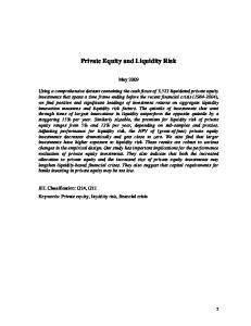
1. Introduction From 2003 to mid-2007, two phenomena grew in parallel on financial markets. Liquidity was at record highs and private equity (PE) firms distributed increasingly large amounts of cash to their investors. These investors in turn were re-investing the cash in newly raised private equity funds and much new money was flowing into the PE industry. Mid-2007, the music stopped. Liquidity suddenly dried up and PE firms hardly distributed any cash to their investors thereafter. Figure 1 illustrates this phenomenon by plotting the monthly pay-out of private equity investments in our data set and the Ted spread1, a commonly accepted measure of liquidity. Strikingly, the run-up and subsequent fall in private-equity pay-outs goes hand in hand with the dramatic drying up of liquidity in the financial system at large. This episode suggests that PE investors may receive higher returns in times of higher liquidity. In light of the recent literature on the pricing of liquidity risk, this fact, if confirmed on a large dataset, would have important consequences for the evaluation of private equity performance and the valuation of private equity investments. Pastor and Stambaugh (2003), Acharya and Pedersen (2005), and Liu (2006), among others, show that (systematic) liquidity risk is priced for public equity and that investors require a sizeable liquidity risk premium for stocks.2 In private equity, the effect may be even more dramatic, because investment exits appear to cluster at times of high IPO and M&A activities, both of which are related to market liquidity (see Cumming, Fleming and Schwienbacher, 2005). That private equity returns may need a sizeable adjustment because of a large exposure to liquidity risk is also highlighted by Metrick (2007). Using an index of venture capital returns and a time-series regression, he estimates a 1% annual premium for liquidity risk. The objective of this paper is to see whether the anecdotal evidence mentioned above and Metrick’s early result hold in a comprehensive dataset of pre-crisis PE investment returns. In addition, the unique depth of our dataset enables us to document which type of investments are most sensitive to liquidity risk. Finally, our data enables us to further document the issue of private equity performance. Previous research finds that private equity buyout funds underperform

1

The Ted spread is defined as the three-month LIBOR rate minus the Fed Funds rate in basis points. Other articles include: Chordia, Subrahmanyam, and Anshuman (2001), Baekert, Harvey, and Lundblad (2005), Watanabe and Watanabe (2008), Martinez, Nieto, Rubio, and Tapia (2005), Bandi, Moise, and Russel (2008), Fontaine and Garcia (2008), and Hasbrouck (2009).

2

3

public equity after fees (Kaplan and Schoar, 2005, Phalippou and Gottschalg, 2009) but the quality of the data is sometimes questioned. Here, we report evidence before fees from a different and detail-rich dataset. Figure 1

1.5

The figure plots the monthly dividend payout of private equity deals in the CEPRES dataset (PE payout) and the monthly Ted spread (defined as the three-month LIBOR rate minus the Fed Funds rate in basis points). Dividend payout is constructed as the six-month moving average of the total dividends paid divided by the six-month moving average of the total investments in those deals. 200

PE payout Ted spread (bp)

.5

100

Ted spread (bp)

PE payout

1

150

20 08

20 07

20 06

20 05

20 04

20 03

0 20 02

20 01

0

50

Our dataset contains detailed cash-flow information for 3,421 PE investments made between 1981 and 2000 (and realized by December 2004) in 32 countries. We do not know the identity of each investment or fund but have information on industry, stage, exit type, and country of the investment. We also have information about fund size and fund sequence number. We first show that investment performance is significantly related to the average innovation in aggregate liquidity during the investment’s lifetime. This result holds for all four non-traded liquidity measures that are available for our sample period (Pastor and Stambaugh, 2003, Acharya and Pedersen, 2005, and Sadka’s, 2006, two measures). Second, we use traded liquidity factors to measure more directly the liquidity risk premium of private equity investments. Depending on the measures applied, the premium ranges from 5% to 15% per year. 4

Third, we investigate which investment characteristics affect the exposure of PE to liquidity risk. Our preliminary analysis suggests that investment size is a positive and significant determinant of exposure to liquidity risk. Larger investments are indeed more sensitive to exit conditions than smaller investments and thus potentially via this channel, more sensitive to liquidity risk. Our study is related to that of Cumming, Fleming and Schwienbacher (2005). They show that venture capitalists invest in different type of companies as a function of market liquidity, which they proxy by the number of IPOs per year. They conclude that their results are “consistent with the view that illiquidity is one reason why venture capitalists require higher returns on their investments”. Our paper also relates to two important strands of literature. First, we connect to the literature on the pricing of liquidity risk.3 A number of papers provide theoretical arguments as to why investors want to be compensated for liquidity risk (e.g. Holmstrom and Tirole, 2001, Acharya and Pedersen, 2005, Lustig, 2009). The empirical literature was pioneered by Amihud and Mendelson (1986) and more recent work emphasizes the importance of systematic liquidity risk in public equity returns (e.g. Amihud, 2002, Pastor and Stambaugh, 2003, Acharya and Pedersen, 2005, Sadka, 2006). Second, we relate to the literature on risk and return of private equity investments (e.g. Cochrane, 2005, Cumming, Schmidt and Walz, 2009, Kaplan and Schoar, 2005, Phalippou and Gottschalg, 2009, Driessen, Lin and Phalippou, 2008, Lerner, Schoar and Wongsunwai, 2007, Jones and Rhodes Kropf, 2003, Ljungqvist, Richardson and Wolfenson, 2007, Hochberg, Ljungqvist and Vissing-Jorgensen, 2008).4 This paper continues as follows. Section 2 describes the data. Section 3 describes the liquidity measures. Section 4 discusses the methodology. Section 5 shows the main empirical results. Section 6 offers some robustness tests and section 7 briefly concludes.

3 4

See Amihud, Mendelson, and Pedersen (2005) for a survey. See Phalippou (2007) for a survey. 5

2. Data 2.1. Data source and comparable datasets The dataset is provided by the Center for Private Equity Research (CEPRES). CEPRES is a private consulting firm established in 2001 as a co-operation between the University of Frankfurt and Sal. Oppenheim Banking Group. CEPRES obtains data from private equity fund managers in exchange for free exclusive access to information services. The data are received through standardized information request sheets. CEPRES then validates the data with due diligence reports, including audited filings, to guarantee accuracy. An earlier version of the CEPRES database covering mainly or exclusively venture capital is used by Cumming and Walz (2004) and Cumming, Schmidt and Walz (2009), respectively. The unique aspect of the dataset is that it contains monthly cash flows for each investment (i.e. Portfolio Company) of a fund. Such a feature is important because it enables us to construct precise performance measures for each investment (IRRs and Modified IRRs), which is essential for accurate estimation of the relation between performance and liquidity risk. The only other database we know of that contains cash flows at the investment level is that of Ljungqvist, Richardson and Wolfenson (2008). Our data spans a longer time period (1981 until 2007 versus 2003) and, in addition, contains more twice as many investments (from 1981 to 2003, they report a total of 2,274 investments while our data set contains 4,401 buyout investments from 1981 to 2007). Importantly, they show descriptive statistics only at the fund level. This means that the descriptive statistics we show below are novel. Another database with cash flow details is provided by Thomson Venture Economics, but it contains this information only at the fund level.5 Having cash flow information at the investment level rather than at the fund level gives us more power to detect a relation between performance and liquidity and enables us to study the interaction between investment characteristics and liquidity exposure. Finally, Lopez-de-Silanes and Phalippou (2009) have a dataset with the performance of a large panel of investments, which comes from hand-collected private placement memoranda (PPMs). They do not have cash flow details for each investment but only a cash multiple and an IRR. The major benefit of our data compared to theirs is that we can compute different performance measures (e.g., Modified IRR) and thus make more precise inferences thanks to the cash flow details. 5

It has been used by Kaplan and Schoar (2005), Phalippou and Gottschalg (2009), Jones and Rhodes-Kropf (2003) and Driessen, Lin and Phalippou (2008). 6

2.2. Sample selection Table 1 shows how we select our sample. To gauge sample bias in performance, we show the mean and median Cash multiple in each sub-sample. Cash multiple is the only performance indicator that we observe for all the investments; it is defined as the total amount distributed divided by the total amount invested.6 CEPRES defines private equity buyout investments according to the following categories: Acquisition financing, Leveraged Buy-Outs (LBO), Management Buy-Outs and Buy-Ins (MBO/MBI), Growth, Recapitalisation, Spin off, and Turnaround. We count 4,401 buyout investments undertaken from 1981 until 2007. As young investments are often held at cost, we focus on investments made between 1981 and 2000. This increases performance precisely because many investments held at cost (hence, with a multiple of 1) are removed. That sample has 3,944 observations and a mean and median performance of 2.60 and 1.93 respectively, compared to 2.59 and 1.95 in the full sample. Next, we select only the investments that are liquidated by December 2004. This is because i) their performance is final (and not influenced by subjective accounting valuations), ii) we have cash flow information only for liquidated investments and iii) we have liquidity factors up until December 2004. The sample size decreases to 3566. Consistent with the conjecture in Phalippou and Gottschalg (2009), funds liquidate their winners more quickly, making the liquidated sample tilted towards winners. The difference in performance is however relatively small in our dataset. Finally, we require information about duration. This is missing for 175 investments. As pointed out by Ljungqvist, Richardson and Wolfenson (2008), the date at which investments are officially written off are often missing in such datasets. Once, we require duration information, many bankrupted investments are excluded and performance increases further. However, the difference in performance between the full sample and the selected sample is relatively small; though we ought to bear in mind that we have a tilt towards better performers. The final sample has 3,421 observations and mean and median multiple of 2.766 and 2.076 respectively. [Insert Table 1 about here]

6

Only the cash multiple in local currency is available to us for all the observations. 7

2.3. Performance Measures Our main performance measure is the Internal Rate of Return (IRR). We compute it on both the cash flows expressed in their original currency and the cash flows converted in US dollars; we label them IRR (local) and IRR (dollar) respectively. The main issue with IRR is that of the re-investment assumption. This means that, if so measured, both the average performance and the dispersion of performance is exaggerated (Phalippou, 2009). However, since we use IRR for a cross-sectional regression, its flaws may not significantly bias our results on factor exposure as the correlation between IRR and effective rate of return is likely to be high. On the other hand, the alphas from these regressions are not meaningful. Hence, we abstain from interpreting a positive (negative) constant in our multifactor regression models with liquidity as out-performance (under-performance) after adjusting for risk factors. The effective rate of return is not observable. For that, we would need to know the reinvestment rate of the representative investor at each point in time. Instead, to gauge whether our results are sensitive to the re-investment assumption, we use two additional performance measures. First, a Modified IRR with a constant 8% re-investment rate and another Modified IRR with the S&P 500 as the re-investment rate. We label them MIRR (8%) and MIRR (S&P), respectively. The first one is computed on the cash flows in the original currency, while the second one is computed on the cash flows converted in US dollars.7 We observe fat tails for all the performance measures. For this reason, we winsorize all of them at the 95th percentile. When converting to monthly returns, the annual IRRs that equal 100% are set to -99% to flatten the left tail of the resulting distribution. Figure 2 shows the final distribution of our performance measures at the annual frequency. [Insert Figure 2 about here] Table 2 shows the correlation between the four performance measures. The correlation is very high which confirms that cross-sectional results will not be significantly affected by the re-investment assumption. The mean and median is however different. The mean IRR is at 23% while the mean Modified IRR is at 10% and 14% when we change the re-investment assumption to 8% and S&P 500 respectively. This shows that only changing the re-investment 7

In a similar context, Ljungqvist et al. (2008) use a Modified IRR with 0% re-investment rate. We will use an 8% re-investment rate and the S&P 500 as a re-investment rate in the robustness section. 8

assumption brings private equity performance close to public equity market returns, gross-offees. Phalippou (2009) estimates fees to be in the range of 6-8% for an investment whose performance matches that of the S&P 500. Net-of-fees, performance thus seems to be rather low. [Insert Table 2 about here]

2.4. Raw performance statistics Table 3 shows the descriptive statistics of our working sample of private equity investments. We convert all cash flows into US dollars, and investment size is expressed in year 2000 US dollars. VW is the (investment-size) value-weighted mean, and DVW is the durationtimes-value-weighted mean. Duration is measured from the first to the last cash flow. Performance measures are cash multiple (total amount distributed divided by total amount invested), Internal Rate of Return (IRR) and Modified IRR with either a flat 8% or S&P 500 index as re-investment rate. Performance and sample distributions are displayed by year (Panel A), by industry (Panel B), by investment stage (Panel C), by exit type (Panel D), and by country (Panel E). [Insert Table 3 about here] Panel A shows that the number of investments starts slowly and then takes off rapidly in the second half of the 1980s peaking to 354 investments in 1997. Median size of investment is almost monotonically increasing throughout most of the sample period. Panel B shows statistics by industry. Most investments are in industrial/manufacturing (640 investments) and consumer/food (359), the traditional private equity industries. A large number of investments are also reported for less traditional industries like healthcare (311) and services (304). Panel C shows that almost three quarter of the number of investment stages are classified as MBOs (2322). Exit channel is provided for about half of the investments. Panel D shows that the majority (1112 exits) are realized through a trade sale. There are only 288 IPO exits. These exits have the highest performance. The second best exit in terms of performance is public merger.

9

3. Liquidity 3.1. Liquidity risk and liquidity level Our paper focuses on the compensation for systematic risk originating from timevarying liquidity. A recent literature in asset pricing has argued that investors prefer assets that pay out $1 in times of low liquidity than in times of high liquidity. The current crisis illustrates clearly these arguments and emphasizes how private equity was particularly sensitive to liquidity risk. Large PE investors (Endowments such as Harvard, Pension funds such as Calpers) would have most probably preferred receiving large dividends from their PE portfolio in 2008 rather than receiving them in 2006 (ex-post). Harvard endowment has tried to sell a staggering $1.5 billion of PE stakes in 2008 in an attempt to receive some cash from its PE division. It failed to sell this stake at a reasonable discount and as of Q1-2009 has not sold it.8 A related topic is the compensation for the level of liquidity, i.e. the level of transaction costs and the trading restrictions associated with PE investments. The only study we are aware of in private equity is that of Lerner and Schoar (2004). They propose a model and supporting empirical evidence which show that the liquidity level of PE funds is a decision variable for the fund managers. Namely fund managers make the fund stakes illiquid on purpose and the degree to which they do it depends on the type of investments the fund makes. Future research may focus on the discount required for the illiquidity level of private equity. Having part of a portfolio in an illiquid asset class can be costly if one needs to sell this

8

Private Equity Online – November 7, 2008: “Harvard Management Company is looking to unload roughly $1.5 billion in private equity stakes in the secondary market. A secondary market source described the university endowment, which had $36.9 billion in assets as of 30 June, as a highly sophisticated limited partner making a proactive decision to seek liquidity and rebalance its portfolio based on cash flow models. Although the volume of supply in the secondary market has risen of late, secondary investors expect it to surge further in the first half of 2009 as more LPs make a similar move to access needed liquidity. Harvard is ahead of many limited partners in going to the secondary market and will obtain a more attractive price for its assets than those heading to market six months down the line as the result of supply demand dynamics, the investor said. Harvard’s secondary sale will drive down prices in the secondaries market because it will take $1.5 billion of demand out of the market at a time when supply is not rising, the investor added.” THEN Bloomberg – January 23, 2009: “Harvard University didn’t sell most of the $1.5 billion of stakes in private-equity funds it put on the market last year because offers were too low, said three people familiar with the matter. The university’s $28.8 billion endowment, the richest in higher education, rejected deals as sellers, including schools and pension funds, flooded the market and pushed down prices, said the people, who asked not to be identified because the bidding is private. The Cambridge, Massachusetts university remains interested in unloading the private-equity investments. Harvard, Duke University and Columbia University were among institutions that last year put buyout and venture capital stakes up for sale on the secondary market, where middlemen broker deals. Schools are looking to raise cash as distributions from fund managers dry up and losses on stocks and bonds mount. As much as $40 billion in private-equity interests may go unsold this year as sellers hold out for higher prices, according to Nyppex Holdings LLC, a firm that trades stakes in buyout pools.” 10

part of the portfolio for whatever reason (like Harvard endowment in the example above). Studying this problem is interesting but needs considerable assumptions and data that we do not have. For example, one needs to conjecture the ex-ante probability that an investor has to sell a given PE stake. Another related issue is that investors effectively grant a credit line to the PE fund. The relation between the speed of draw down and the liquidity of the rest of an investor’s portfolio is then crucial to evaluate the cost of this credit line.

3.2 Liquidity measures Non-traded Market-wide Liquidity Measures The literature has proposed several measures of shocks to aggregate (market-wide) liquidity. We use the four measures that are available for our sample period. First, we use the (innovation in the) aggregate liquidity measure of Pastor and Stambaugh (2003), which we denote PS-LIQ. It is the aggregate of firm-level (OLS) coefficients of daily returns on signed daily trading volume. Our second measure is the innovation in market illiquidity as computed by Acharya and Pedersen (2005), where the firm-level illiquidity is measured by the ratio of Amihud (2002). We multiply this measure by minus one to obtain a liquidity measure and denote it AP-LIQ. Third and fourth, we apply the measures of Sadka (2006). He proposes a measure of market-wide price impact, which he decomposes in a permanent (variable) and a transitory (fixed) part, which we label Sadka-pv and Sadka-tf, respectively.

Traded Liquidity Risk Factors We also choose all the traded liquidity factors proposed in the literature that are available for our sample time period. First, Pastor and Stambaugh (2003) have created two time-series of long-short portfolios. One is equally weighted and the other is value-weighted; we denote them IML_ew_PS and IML_vw_PS, respectively. We should keep in mind that Pastor and Stambaugh privilege the equally-weighted measure in their paper. They argue that it is a more stable measure. Second, Liu (2006) proposes a liquidity measure for individual stocks which is a standardized turnover-adjusted number of zero daily trading volumes over the prior 12 months. Stocks are then assigned to deciles as a function of their liquidity. The return on the low deciles minus the return on the high deciles portfolio is the mimicking liquidity factor.

11

3.3. Descriptive statistics Table 4 shows the cross-correlation and distribution of the pricing factors and aggregate liquidity factors. The table shows the correlation matrix for the (time-series of the) six pricing factors (the usual three factors Rm-Rf, HML, SMB, and three illiquid minus liquid factors) plus the four aggregate measures of liquidity. Time period is from January 1981 to December 2004. [Insert Table 4 about here] The Liu liquidity factor returns a high 0.91% per month. Pastor and Stambaugh factors return 0.56% and 0.40% per month. The liquidity measures have zero mean by construction. We also note that the liquidity measures and factors are not highly correlated with one another. They capture different dimensions of liquidity. Consequently, it is important to show results with all the measures. Also of interest, the Liu factor is highly correlated with HML. Hence, as in Liu (2006) we will use his factor only in addition to the market factor (a two-factor model). In contrast, Pastor and Stambaugh (2003) use their factor in addition to the three Fama-French factors. The four factors have low correlation with one another. In sub-sequent analysis, we will also use this four factor model.

4. Methodology For each investment, we observe all the cash flows. To begin, let us assume that each investment i consists of only one negative cash flow (I) and one positive cash flow (D). Let us further assume a two factor model as in Liu (2006), in which the factors are the market risk premium (rmt - rft) and the liquidity risk premium (LIQt). Denoting ut the idiosyncratic shocks, it follows from standard asset pricing theory that: ∏

1

,

,

)

,

Dividing by I and taking the natural logarithm on both sides gives

ln 1

,

ln

1

,

,

,

12

Which we can approximate by the following (we work at a monthly frequency):

,

,

,

,

or ,

,

,

,

,

This approximation can be avoided by making a distributional assumption. Assuming the ut are normally distributed or lognormally distributed, then maximum likelihood can be used. Alternatively, techniques such as that of Driessen, Lin and Phalippou (2008) can be used here. We leave these alternative estimation approaches as a robustness test for future versions. The other assumption we made here is that of no intermediary cash flows. In the analysis that follows we use IRR and two modified IRR to proxy for Ri,t and thereby gauging whether the existence of intermediary dividends significantly affect results. In the next version, we will also create factors mimicking IRRs to further judge the sensitivity of results to the presence of intermediary cash flows.

5. Empirical Results 5.1. Non-traded Market-wide Liquidity Measures Table 5 shows the result of OLS regressions of PE returns on (non-traded) market-wide liquidity factors. Standard errors are based on a three dimensional clustering (month/year of the investment, fund country and investment industry); and corresponding t-statistics are reported below each coefficient in italics. Dependent variables include the usual three asset pricing factors and four aggregate (market-wide) liquidity measures. Each dependent variable is the time-series average during the investment’s life of the corresponding variable. The results on the non-traded aggregate liquidity factors are all significant at conventional levels. In simple regressions (specs 1, 4 and 10) the effect is largest. As the other risk factors, such as the excess return on the market, HML, and SMB are correlated with the liquidity variables, the marginal effect of liquidity decreases (but remains significant) when these factors are added to the regressions. Hence, we find that PE returns are sensitive to systematic liquidity risk. [Insert Table 5 about here] 13

5.2. Traded Liquidity Risk Factors Table 6 shows the result of OLS regressions of PE returns on traded liquidity risk factors. Again, standard errors are based on a three dimensional clustering (month/year of the investment, fund country and investment industry), and corresponding t-statistics are reported below each coefficient in italics. Dependent variables include the usual three asset pricing factors and three zero-cost illiquid minus liquid portfolios (i.e. traded liquidity risk factors). Each dependent variable is the time-series average during the investment’s life of the corresponding variable. The traditional one factor model (spec 1) shows that private equity returns are positively related to public equity return (beta is 1.7). Next, we show results with the two-factor model of Liu (2006). We find a very large effect of the liquidity factor. It is significant at the 1% level test and the economic magnitude is very large. The average IML of Liu is 0.91% per month (see table 4), making a liquidity premium of 1.17% per month or 15% per year. Next, in specification 3, we adopt the three-factor model of Fama and French (1993). The evidence suggests that private equity returns, as commonly believed, co-move positively and significantly with the returns on value stocks. Next, in specifications 4 and 5, we show results for a four-factor model that includes Pastor and Stambaugh’s (2003) liquidity factor. The effect is significant only for the equally-weighted measure, which is the one favored by Pastor and Stambaugh (2003). Under this measure the annual liquidity premium is 5.3%. [Insert Table 6 about here]

5.3. Abnormal Performance We now go back to the evidence on private equity performance that we discussed above. We have shown raw performance numbers. Now that we have measures of risk, it is interesting to measure the decrease in NPV due to risk correction and, in particular to liquidity risk. Results are shown in Table 7. We display the average NPV across vintage years and the average Profitability Index across vintage years (present value of aggregated dividends divided by present value of aggregated investments). We also show the NPV and PI on the aggregated cash flows (all vintage years pooled together).

14

We begin by discounting with a beta of one on the market factor. We find a large PI and positive NPV. Next, we show the result for the two factor model of Liu if we set the market beta to one and if we set it to 2.35 (as estimated in Table 6). We observe that both the NPV and PI decrease significantly. After market risk and liquidity risk correction, PI on the aggregate cash flow is only 1.06. This means that gross of fees, the value created is 6% of the value invested (for the whole investment’s life). Metrick and Yasuda (2008) estimate fees to be about 20% in present value terms, which means that net of fees, and after risk adjustment, it is a deeply negative NPV investment for PE fund investors. We repeat the same exercise with the Pastor and Stambaugh measure. Consistent with a lower liquidity premium with this measure, we find a higher PI and NPV. But the results are qualitatively the same as those above. [Insert Table 7 about here]

5.4. Investment characteristics and exposure to liquidity risk Next, we investigate which investment characteristics affect the exposure of PE to liquidity risk. Results in Table 8 suggests that investment size is a positive and significant determinant of exposure to liquidity risk. Larger investments are indeed more sensitive to exit conditions than smaller investments and thus potentially via this channel, more sensitive to liquidity risk. [Insert Table 8 about here]

6. Robustness 6.1. US versus non-US In this version, we have used only US liquidity factors. As pointed out by Bekaert, Harvey and Lundblad (2007) liquidity risk is mainly local. Although their results are on emerging markets, we expect a similar situation for European countries (roughly half of our sample). In the next version, we plan on using global and local liquidity risk measures. In this version, we show results separately for the sub-sample of US and non-US investments. Table 9 shows the sub-sample of US investments. The Pastor and Stambaugh measure is stronger economically and statistically. The liquidity premium raises to 11.5% per year. The 15

liquidity premium of Liu stays the same at about 15% per year. The aggregate liquidity measures of Sadka are not significant on this sub-sample, the other two stays significant. In the non-US sample, the Pastor and Stambaugh measure is not significant while the Liu measure remains significant and of the same order of magnitude. All aggregate liquidity measures are significant except Acharya-Pedersen. Results are similar if we use local currencies to compute performance. [Insert Table 9 about here]

6.2. Modified IRR As pointed out above, IRR suffers from a re-investment assumption and our approach was an approximation given the existence of intermediary cash flows. We changed the assumption on the re-investment rate. We use either a flat 8% or the S&P 500 and in either case, we find that the results are very similar (Table 10). This gives credit to our performance measure and to the accuracy of the liquidity risk premium we estimate. [Insert Table 10 about here]

7. Conclusion Using a comprehensive dataset containing the cash flows of 3,421 liquidated private equity investments made between 1981 and 2000, we find positive and significant loadings of investment returns on aggregate liquidity innovation measures and liquidity risk factors. The premium for liquidity risk of private equity is up to 15% per year. After adjusting performance for liquidity risk, (gross-of-fees) private equity investments have an NPV close to zero. We also find that larger investments have higher exposure to liquidity risk. These results are robust to various changes in the empirical design. Our study has important implications for the performance evaluation of private equity investments.

16

References Acharya, Viral V., and Lasse Heje Pedersen, 2005, Asset Pricing with Liquidity Risk. Journal of Financial Economics, 77: 375-410. Amihud, Yakov, 2002, Illiquidity and Stock Returns: Cross-Section and Time-Series Effects. Journal of Financial Markets, 5(1): 31-56. Amihud, Yakov, and Haim Mendelson, 1986, Asset Pricing and the Bid-Ask Spread. Journal of Financial Economics, 17: 223-249. Amihud, Yakov, Haim Mendelson, and Lasse Heje Pedersen, 2005, Foundations and Trends in Finance, 1(4): 269-364. Bandi, Federico M., Claudia E. Moise, and Jeffrey R. Russell, 2008, The Joint Pricing of Volatility and Liquidity. Working Paper, Chicago Booth and Case Western. Bekaert, Geert, Campbell Harvey, and Christian Lundblad, 2007, Liquidity and Expected Returns: Lessons from Emerging Markets. Review of Financial Studies, 20(6): 17831831. Chordia, Tarun, Avanidhar Subrahmanyam, and V. Ravi Anshuman, 2001, Trading Activity and Expected Stock Returns. Journal of Financial Economics, 59: 3-32. Cochrane, John, 2005, The Risk and Return of Venture Capital. Journal of Financial Economics, 75: 3-52. Cumming, Douglas J., 2008. Contracts and Exits in Venture Capital Finance. Review of Financial Studies, 21(5): 1947-1982. Cumming, Douglas J., Grant Fleming and Armin Schwienbacher, 2005, Liquidity Risk and Venture Capital Finance. Financial Management, 34: 77-105. Cumming, Douglas J., Daniel Schmidt, and Uwe Walz, 2009, Legality and Venture Capital Governance around the World. Journal of Business Venturing, forthcoming. Cumming, Douglas, and Uwe Walz, 2004, Private Equity Returns and Disclosure around the World. Working Paper, EFA 2004 Maastricht. Driessen, Joost, T. Chun Lin, and Ludovic Phalippou, 2008, A New Method to Estimate Risk and Return of Non-Traded Assets from Cash Flows: The Case of Private Equity Funds. NBER Working Paper 14144. Fontaine, Jean-Sebastien and Garcia, Rene, 2008, Bond Liquidity Premia. SSRN Working Paper 966227. Gompers, Paul A. and Josh Lerner, 2000, Money Chasing Deals: The impact of fund inflows on 17

private equity valuations. Journal of Financial Economics, 55: 281–325. Hasbrouck, Joel, 2009, Trading Costs and Returns for US Equities: Estimating Effective Costs from Daily Data, Journal of Finance, forthcoming. Hochberg, Yael V., Alexander Ljungqvist, and Annette Vissing-Jorgensen, 2008, Informational Hold-up and Performance Persistence in Venture Capital. Working Paper. Hochberg, Yael V., Alexander Ljungqvist, and Lu Yang, 2007, Whom You Know Matters: Venture Capital Networks and Investment Performance. Journal of Finance, 62 (1), 251301. Holmström, Bengt, and Jean Tirole, 2001, LAPM: A Liquidity-Based Asset Pricing Model. Journal of Finance, 56 (5): 1837-1867. Jones, Charles, and Matthew Rhodes-Kropf, 2004, The Price of Diversifiable Risk in Venture Capital and Private Equity. Working Paper, Columbia University. Kaplan, Steve and Antoinette Schoar, 2005, Private Equity Performance: Returns, Persistence and Capital Flows. Journal of Finance, 60: 1791-1823. Kaplan, Steve N., Berk A. Sensoy and Per Strömberg, 2002, How well do venture capital databases reflect actual investments? Working Paper, University of Chicago. Lerner, Josh, Antoinette Schoar, and Wan Wongsunwai, 2007, Smart Institutions, Foolish Choices? The Limited Partner Performance Puzzle. Journal of Finance, 62 (2): 731-764. Lopez De Silanes, Florencio, and Ludovic Phalippou, 2009, Private Equity Investments: Performance and Diseconomies of Scale. Working Paper. Liu, Weimin, 2006, A Liquidity-Augmented Capital Asset Pricing Model. Journal of Financial Economics, 82: 631–671. Ljungqvist, Alexander and Matthew Richardson, 2003, The Cash Flow, Return and Risk Characteristics of Private Equity. Working Paper, NYU Stern School of Business. Ljungqvist, Alexander, Matthew Richardson, and Daniel Wolfenzon, 2008, The Investment Behavior of Buyout Funds, NBER Working Paper W14180. Lustig, H., 2009. The Market Price of Aggregate Risk and the Wealth Distribution. NBER Working Paper W11132. Martínez, Miguel A., Belén Nieto, Gonzalo Rubio, and Mikel Tapia, 2005, Asset Pricing and Systematic Liquidity Risk: An Empirical Investigation of the Spanish Stock Market. International Review of Economics and Finance, 14: 81-103. Metrick, Andrew, 2007, Venture Capital and the Finance of Innovation, Wiley & Sons. 18

Metrick, Andrew and Yasuda, Ayako, 2008, The Economics of Private Equity Funds, Swedish Institute for Financial Research Conference on The Economics of the Private Equity Market. Available at SSRN: http://ssrn.com/abstract=996334. Pástor, Lubos and Robert F. Stambaugh, 2003, Liquidity Risk and Expected Stock Returns. Journal of Political Economy, 111(3): 642-685. Petersen, Mitchell A., 2009, Estimating Standard Errors in Finance Panel Data Sets: Comparing Approaches. Review of Financial Studies, 22(1): 435-480. Phalippou, Ludovic, 2009, Beware of Venturing into Private Equity, Journal of Economic Perspectives, 23(1): 147–66. Phalippou, Ludovic and Oliver Gottschalg, 2009, The Performance of Private Equity Funds. Review of Financial Studies, forthcoming. Sadka, Ronnie, 2006, Momentum and Post-Earnings-Announcement Drift Anomalies: The Role of Liquidity Risk. Journal of Financial Economics, 80: 309-349. Watanabe, Akiko and Masahiro Watanabe, 2008, Time-Varying Liquidity Risk and the Cross Section of Stock Returns. Review of Financial Studies, 21 (6): 2449-2486.

19

Table 1: Sample selection and Performance This table shows the (equally weighted) mean and median cash multiples. Cash multiple is the total amount distributed divided by total amount invested. All cash flows are in local currency. Liquidated investments are those officially liquidated as of December 2004. Some investments (mainly written-offs) do not have information about duration. Cash Multiple (local currency) Mean Median All buyout investments (1981-2007) All buyout investments (1981-2000) Liquidated buyout investments (1981-2000) Working sample: Liquidated buyout investments (1981-2000) with duration information

N_obs

2.593 2.607 2.654

1.952 1.933 1.958

4401 3944 3566

2.766

2.076

3421

20

Table 2: Correlation and distribution of performance measures This table shows the correlation matrix for the natural logarithm of duration plus five performance measures. Performance measures are winsorized at the 95th percentile. Mean is value weighted by deflated investment size expressed in US dollar. The distribution of each variable is displayed underneath the correlation matrix. * denotes that the performance is computed on cash flows in local currency.

Duration IRR* IRR MIRR_8% MIRR_S&P Multiple Mean (VW) Median St. Deviation 5th percentile 95th percentile

Duration

IRR*

IRR

MIRR_8%

MIRR_S&P

Multiple

1.000 -0.126 -0.129 -0.094 -0.087 0.067

1.000 0.998 0.937 0.928 0.740

1.000 0.938 0.924 0.740

1.000 0.978 0.717

1.000 0.709

1.000

51.765 49.000 29.049 12.300 117.000

0.216 0.252 0.770 -1.000 2.047

0.231 0.261 0.778 -1.000 2.096

0.095 0.173 0.529 -0.956 1.216

0.143 0.201 0.511 -0.842 1.294

2.441 2.076 2.733 0.000 10.174

21

Table 3: Descriptive statistics This table shows the descriptive statistics for our working sample. All cash flows are converted in US dollars. Investment size is expressed in 2000 US dollars. VW is value-weighted using investment size and DVW is duration-times-value-weighted. Duration is measured from first to last cash flow. Performance measures are cash multiple (total distributed divided by total invested), Internal Rate of Return and Modified IRR with either a flat 8% or S&P 500 index as reinvestment rate. Performance and sample distribution are displayed by year (Panel A), by industry (Panel B), by investment stage (Panel C), by exit type (Panel D), by country (Panel E). Panel A: Performance per year Year

Size N_obs Median

1981 1982 1983 1984 1985 1986 1987 1988 1989 1990 1991 1992 1993 1994 1995 1996 1997 1998 1999 2000

8 0.484 10 0.681 17 0.835 19 2.223 49 2.449 72 2.164 107 1.788 160 1.565 141 2.743 194 3.081 238 3.738 249 4.503 239 4.269 375 4.620 300 6.777 345 6.876 354 8.773 251 11.906 218 10.399 220 6.046

Mutiple Median Mean VW 0.576 5.216 0.180 4.768 0.435 3.906 4.106 5.480 2.834 3.887 2.672 3.445 1.443 2.254 1.523 2.561 1.508 3.484 1.695 2.735 2.817 2.851 2.178 2.578 2.628 2.940 2.394 2.771 1.822 2.373 1.848 2.447 1.870 2.450 1.758 1.804 1.147 1.649 0.215 1.021

Median -0.074 -0.222 -0.183 0.362 0.463 0.262 0.110 0.104 0.121 0.147 0.346 0.278 0.424 0.326 0.212 0.252 0.307 0.195 0.067 -0.544

IRR Mean Mean VW DVW 0.017 0.073 0.433 0.250 0.181 -0.017 0.561 0.514 0.731 0.285 0.247 0.135 0.304 0.143 0.336 0.217 0.157 0.181 0.318 0.219 0.372 0.285 0.295 0.248 0.432 0.322 0.427 0.405 0.224 0.209 0.294 0.195 0.238 0.275 0.003 0.035 -0.066 0.115 -0.359 -0.001

MIRR_8% Mean VW -0.072 0.029 -0.211 0.224 -0.151 0.128 0.245 0.245 0.252 0.444 0.187 0.085 0.065 0.188 0.079 0.240 0.094 0.099 0.110 0.208 0.220 0.244 0.190 0.184 0.269 0.260 0.214 0.151 0.158 0.132 0.172 0.162 0.204 0.069 0.174 -0.058 0.059 -0.118 -0.506 -0.382

Median

Mean DVW 0.080 0.106 0.063 0.191 0.197 0.085 0.069 0.122 0.118 0.124 0.181 0.144 0.175 0.143 0.121 0.099 0.103 -0.014 0.060 -0.036

MIRR_S&P Median Mean Mean VW DVW -0.053 0.139 0.171 -0.117 0.316 0.213 -0.014 0.245 0.201 0.280 0.321 0.281 0.311 0.518 0.277 0.257 0.145 0.162 0.136 0.227 0.116 0.121 0.295 0.186 0.141 0.167 0.185 0.153 0.277 0.197 0.271 0.295 0.240 0.229 0.248 0.223 0.349 0.328 0.233 0.263 0.242 0.232 0.170 0.194 0.179 0.184 0.243 0.168 0.187 0.102 0.131 0.149 -0.011 0.028 0.058 -0.133 0.051 -0.520 -0.385 -0.032

Panel B: Per industry Industry Industrial/Manufacturing Consumer industry/Food Healthcare/LS Other Services Software Retail Media IT Telecom Financial Services Internet Leisure Semiconductor Materials Textiles Business Services Construction Natural Resources/Energy HighTech Logistics Transportation Traditional products Hotel Waste/Recycling Environment

Size N_obs Median 640 4.996 359 6.393 311 3.746 304 5.457 279 1.243 201 7.668 190 11.606 172 3.505 134 4.761 118 6.203 66 4.784 66 4.852 63 8.430 58 4.305 56 6.632 49 7.354 47 5.967 39 8.127 38 4.509 37 7.923 29 5.688 22 4.707 18 6.766 10 6.469 5 1.609

Mutiple Median Mean VW 1.844 1.944 1.670 1.994 2.083 2.092 2.325 2.127 2.193 2.522 0.088 3.007 1.333 1.826 1.096 1.846 2.876 2.101 1.072 2.618 2.570 1.666 1.776 1.590 0.127

2.479 2.468 2.469 1.902 3.121 2.947 2.547 1.974 1.747 2.032 1.061 2.818 1.885 2.575 1.562 2.388 3.008 1.914 2.233 2.347 2.663 1.822 2.081 1.997 0.258

IRR Median Mean Mean VW DVW 0.207 0.237 0.171 0.232 0.287 0.243 0.333 0.262 0.232 0.397 -0.754 0.631 0.107 0.195 0.015 0.364 0.355 0.294 0.020 0.334 0.392 0.156 0.217 0.342 -0.875

0.235 0.240 0.202 0.224 0.192 0.200 0.042 0.064 0.328 0.284 0.277 0.303 0.296 0.299 -0.070 0.329 -0.249 0.089 -0.002 0.216 -0.397 0.039 0.436 0.479 0.133 0.136 -0.028 0.100 0.009 0.128 0.357 0.287 0.799 0.685 0.130 0.079 0.376 0.428 0.173 0.201 0.350 0.318 0.045 0.069 0.194 0.169 0.615 0.455 -0.806 -0.810

MIRR_8% Median Mean Mean VW DVW 0.158 0.170 0.109 0.163 0.193 0.162 0.201 0.140 0.157 0.207 -0.691 0.296 0.066 0.116 0.015 0.214 0.298 0.239 0.018 0.273 0.198 0.111 0.157 0.226 -0.825

0.081 0.100 0.110 -0.013 0.119 0.126 0.173 -0.215 -0.300 -0.081 -0.445 0.193 0.064 -0.040 -0.089 0.218 0.311 0.098 0.066 0.063 0.217 0.052 0.177 0.282 -0.698

0.088 0.126 0.115 0.017 0.095 0.156 0.181 0.122 0.022 0.112 -0.053 0.207 0.059 0.131 -0.011 0.145 0.243 0.069 0.095 0.147 0.183 0.067 0.153 0.146 -0.666

MIRR_S&P Median Mean Mean VW DVW 0.179 0.194 0.142 0.189 0.215 0.205 0.233 0.208 0.221 0.257 -0.626 0.422 0.098 0.177 0.081 0.237 0.304 0.224 0.027 0.286 0.280 0.137 0.209 0.249 -0.288

0.140 0.149 0.140 0.061 0.157 0.169 0.213 -0.200 -0.272 -0.052 -0.414 0.274 0.136 -0.002 -0.011 0.285 0.418 0.140 0.146 0.085 0.250 0.089 0.184 0.303 -0.413

0.153 0.173 0.154 0.104 0.142 0.193 0.222 0.148 0.072 0.155 -0.012 0.293 0.125 0.191 0.083 0.209 0.337 0.111 0.166 0.174 0.239 0.104 0.151 0.202 -0.274

23

Panel C: Per investment stage Investment stage

Size N_obs Median

MBO/MBI Growth LBO Acquisition Financing Recapitalisation Turnaround Spin Off

Mutiple Median Mean VW

2322 6.618 806 1.433 184 7.031 110 13.074 105 4.620 33 5.042 6 2.710

1.983 1.384 2.732 2.080 2.230 1.618 0.109

2.213 2.133 2.775 2.544 2.824 1.185 0.804

IRR Median Mean Mean VW DVW 0.253 0.102 0.305 0.312 0.315 0.174 -0.883

0.155 0.207 0.033 0.132 0.180 0.237 0.430 0.369 0.223 0.273 0.025 -0.085 -0.681 -0.834

MIRR_8% Median Mean Mean VW DVW 0.180 0.077 0.217 0.205 0.176 0.148 -0.706

0.034 -0.056 0.109 0.280 0.099 -0.038 -0.608

0.087 0.043 0.161 0.238 0.164 -0.105 -0.664

MIRR_S&P Median Mean Mean VW DVW 0.205 0.104 0.237 0.218 0.242 0.149 -0.627

0.081 0.009 0.125 0.327 0.157 -0.018 -0.496

0.142 0.112 0.183 0.278 0.222 -0.076 -0.502

Panel D: Per exit channel Exit channel Sale Write off IPO Public merger

Size N_obs Median 1112 420 288 73

6.307 4.549 8.182 7.614

Mutiple Median Mean VW 2.061 0.000 3.528 3.264

2.443 0.023 3.599 2.517

IRR Median Mean VW

Mean DVW

MIRR _8% Median Mean Mean VW DVW

MIRR _S&P Median Mean Mean VW DVW

0.286 0.315 0.248 -1.000 -0.984 -0.975 0.599 0.543 0.417 0.355 0.408 0.393

0.213 0.196 0.145 -0.997 -0.922 -0.813 0.395 0.332 0.237 0.254 0.191 0.181

0.230 0.231 0.183 -0.999 -0.800 -0.555 0.432 0.376 0.293 0.290 0.252 0.227

24

Table 4: Correlation and distribution of the factors This table shows the correlation matrix for the (time-series of the) six traded factors (market premium, value premium, size premium and three illiquid minus liquid factors) plus the four aggregate measures of liquidity. The time period is from January 1981 to December 2004. The frequency is monthly.

Rm-Rf HML SMB IML_Liu IML_ew_PS IML_vw_PS PS_LIQ AP_Liq Sadka_tf Sadka_pv Mean Median St. Deviation 5th percentile 95th percentile

Rm-Rf 1.000 -0.503 0.186 -0.751 -0.110 -0.095 0.330 0.090 -0.047 0.108

HML

SMB

IML_Liu

IML_ew_PS IML_vw_PS

1.000 -0.432 0.683 -0.230 -0.184 -0.062 0.020 0.142 -0.002

1.000 -0.292 0.135 0.187 0.037 0.114 0.090 0.114

1.000 0.061 0.025 -0.170 0.030 0.246 0.058

1.000 0.777 -0.003 0.000 -0.005 0.080

0.594 1.030 4.478 -6.910 7.100

0.500 0.405 3.220 -4.220 5.630

0.123 -0.010 3.337 -4.330 4.890

0.910 1.305 4.057 -6.109 7.504

0.559 0.873 4.559 -7.303 5.930

PS_LIQ

AP_Liq

Sadka_tf

Sadka_pv

1.000 -0.035 0.010 0.030 0.044

1.000 0.061 0.084 0.226

1.000 0.217 0.183

1.000 0.187

1.000

0.401 0.466 5.301 -6.948 7.281

0.002 0.008 0.048 -0.068 0.061

-0.012 -0.015 0.166 -0.260 0.255

0.000 0.000 0.002 -0.003 0.003

0.000 0.001 0.006 -0.010 0.007

25

Table 5: Private Equity Returns and Market-wide Liquidity This table shows the result of OLS pooled panel regression. Standard errors are based on a three dimensional clustering (month/year of the investment, fund country and investment industry); corresponding t-statistics are reported below each coefficient in italics. Dependent variables include the usual three asset pricing factor (market premium, value premium, size premium) and four aggregate (market-wide) liquidity measures. Each dependent variable is the time-series average during investment’s life of the corresponding variable.

PS_LIQ

spec 1 1.422 7.380

spec 2 0.947 3.680

spec 3 0.930 3.570

AP_LIQ

spec 4

0.268 4.080

Dependent variable: IRR in US dollar spec 5 spec 6 spec 7 spec 8

0.182 2.720

spec 9

15.553 2.160

15.507 2.280

-0.003 -1.980

-0.009 -3.530

1.492 2.930 0.633 1.510 0.304 0.720 -0.015 -3.000

3421 0.039

3421 0.045

3421 0.047

HML SMB Constant

N_obs Adj. R-square

1.563 6.390

0.008 3.010 3421 0.012

spec 12

15.699 4.210

9.331 2.410 1.484 5.830

-0.001 -0.440

-0.011 -4.740

7.946 1.970 1.873 4.010 0.501 1.170 0.100 0.230 -0.015 -3.230

3421 0.016

3421 0.040

3421 0.041

14.837 1.730

Sadka_pv 0.967 3.060

spec 11

0.159 2.180

Sadka_tf

Rm-Rf

spec 10

-0.006 -1.530

1.965 4.210 0.536 1.210 0.118 0.270 -0.011 -1.670

1.697 7.080

-0.003 -1.460

-0.015 -5.630

1.734 3.540 0.160 0.320 -0.189 -0.410 -0.015 -3.400

3421 0.040

3421 0.041

3421 0.005

3421 0.040

3421 0.040

26

Table 6: Private Equity Returns and Traded Liquidity Risk Factors This table shows the result of OLS pooled panel regression. Standard errors are based on a three dimensional clustering (month/year of the investment, fund country and investment industry); corresponding t-statistics are reported below each coefficient in italics. Dependent variables include the usual three asset pricing factor (market premium, value premium, size premium) and three zero-cost illiquid minus liquid portfolios (i.e. traded liquidity risk factors). Each dependent variable is the time-series average during investment’s life of the corresponding variable. Dependent variable: IRR in US dollar spec 2 spec 3 spec 4 spec 5 1.292 4.120 0.769 2.450 0.558 1.550 1.698 2.352 2.221 2.261 2.233 7.070 8.380 5.240 5.280 5.240 0.719 1.507 1.096 1.740 3.020 2.230 0.177 0.459 0.235 0.410 1.050 0.540 -0.013 -0.027 -0.019 -0.023 -0.021 -5.450 -6.220 -4.150 -4.720 -4.270

spec 1 IML_Liu IML_ew_PS IML_vw_PS Rm-Rf HML SMB Constant

N_obs Adj. R-square

3421 0.035

3421 0.049

3421 0.037

3421 0.042

3421 0.040

27

Table 7: Abnormal Performance of Private Equity Investments The table reports Net Present Value (NPV) and Profitability Index (PI) with different discount rates. The sample is all liquidated investments made between 1981 and 2000. Each performance measure is computed either as a size-weighted (VW) average of the measure for each investment-year in the sample or aggregating all the cash flows in the sample (Agg.). The NPV is computed using the sum of the cash flows in each month of the relevant investment period and is expressed in million of US dollars. The monthly discount rate in the NPV is the sum of one, the risk free rate in the month, and the products of the risk loadings times the realization of the risk factors in the month. The profitability index is the ratio of the discounted value of the aggregate dividends over the discounted value of the aggregate investments.

Risk exposures

Abnormal PE performance

βcapm

βLiu

βsmb

βhml

βew_PS

NPV (VW)

PI (VW)

Agg. NPV

Agg. PI

1.00

0.00

0.00

0.00

0.00

2.45E+09

1.84

5.31E+09

1.78

1.00 2.35

1.23 1.23

0.00 0.00

0.00 0.00

0.00 0.00

7.73E+08

1.32

4.51E+08

1.31

4.75E+08

1.14

6.89E+07

1.06

1.00

0.00

0.00

0.00

0.77

1.00 2.26

0.00 0.00

0.46 0.46

1.51 1.51

0.77 0.77

2.98E+09 1.28E+09

1.84 1.42

1.83E+09 3.29E+08

1.75 1.46

1.13E+09

1.28

7.31E+07

1.16

28

Table 8: Risk exposure as a function of size The table reports estimates from pooled regressions with IRR (based on US dollar cash flows) as dependent variable. Where indicated, the factors are multiplied by deflated US dollar investment size. Also, where indicated, the factors are multiplied by both investment year dummies and the investment size. Panel A: Traded factors

Liquidity factor Liquidity factor * Size Size Rm-Rf Rm-Rf * Size

-0.051 -0.940 1.606 6.040 0.005 0.840

-0.049 -0.380 2.151 4.470 0.005 0.400 0.839 1.830 -0.004 -0.360 -0.003 -0.010 0.010 0.960

No 3421 0.035

No 3421 0.038

HML HML * Size SMB SMB * Size

Year * factors N_obs Adj. R-square

IML_Liu 0.137 1.266 7.001 0.440 3.510 2.120 -0.006 0.003 0.008 -0.750 0.260 0.830 -0.021 -0.090 -0.155 -0.220 -0.630 -1.220 2.220 5.937 6.880 2.840 0.008 0.011 0.960 1.370

No 3421 0.001

No 3421 0.049

Yes 3421 0.106

0.675 2.860 0.005 2.750 -0.038 -0.790

No 3421 0.016

IML_ew_PS -0.018 0.520 -0.060 1.490 0.007 0.011 2.500 1.840 -0.002 -0.128 -0.030 -1.050 1.656 2.138 4.920 4.410 -0.004 0.009 -0.450 0.770 1.225 2.160 0.017 1.140 0.351 0.720 0.002 0.190

1.501 1.070 0.009 1.490 -0.174 -1.420 0.773 0.460 0.014 1.220 1.639 0.510 0.021 1.540 -0.162 -0.110 0.004 0.380

0.718 2.350 0.005 1.920 -0.070 -1.450

No 3421 0.037

Yes 3421 0.110

No 3421 0.010

No 3421 0.044

IML_vw_PS -0.008 0.440 -0.020 1.100 0.006 0.005 1.960 0.640 -0.034 -0.097 -0.580 -0.670 1.634 2.132 5.550 4.420 0.000 0.008 0.070 0.630 1.073 1.930 0.004 0.210 0.096 0.200 0.007 0.700

-0.417 -0.380 0.008 1.300 -0.186 -1.430 -0.192 -0.110 0.015 1.250 -2.536 -1.260 0.017 1.210 0.655 0.420 0.007 0.640

No 3421 0.036

Yes 3421 0.113

No 3421 0.040

29

Panel B: Non-traded factors Liquidity factor

1.279 6.130 Liquidity factor * Size 0.008 2.940 Size 0.027 0.660 Rm-Rf Rm-Rf * Size HML HML * Size SMB SMB * Size

Years * factors N_obs Adj. R-square

PS_LIQ 0.734 0.722 2.640 2.570 0.015 0.013 2.330 2.100 0.103 0.115 1.430 1.100 1.130 1.660 3.220 2.950 -0.013 -0.014 -1.350 -1.330 0.726 1.560 -0.005 -0.430 0.171 0.370 0.003 0.320

No No 3421 3421 0.040 0.048

No 3421 0.049

AP_LIQ 0.099 0.080 1.330 1.010 0.007 0.006 3.260 3.060 0.268 0.315 2.570 1.960 1.555 1.979 5.730 3.800 -0.001 -0.007 -0.200 -0.590 0.641 1.320 -0.008 -0.740 -0.029 -0.060 0.001 0.140

0.666 0.730 0.010 1.600 -0.016 -0.130 0.058 0.040 -0.002 -0.160 -1.687 -1.070 0.006 0.520 -0.364 -0.220 0.008 0.760

0.176 2.440 0.007 3.740 0.243 2.840

Yes 3421 0.106

No No 3421 3421 0.018 0.045

No 3421 0.046

1.024 3.140 0.006 3.440 0.173 1.930 0.486 0.340 0.002 0.210 -1.645 -1.180 0.003 0.330 -2.225 -1.400 0.004 0.460

16.271 2.050 -0.020 -0.070 -0.092 -1.350

Yes 3421 0.109

No 3421 0.006

Sadka_tf 15.468 15.607 2.070 1.650 0.031 -0.136 0.120 -0.350 -0.067 -0.095 -1.060 -0.740 1.603 1.619 6.060 2.920 0.005 0.010 0.860 0.660 0.238 0.430 0.001 0.100 -0.400 -0.760 0.014 0.880

23.859 0.750 -0.143 -0.360 -0.118 -0.940 -0.197 -0.120 0.012 0.790 -2.668 -1.360 0.009 0.600 -0.480 -0.230 0.013 0.780

12.649 3.120 0.265 4.170 -0.084 -2.150

No 3421 0.040

Yes 3421 0.108

No 3421 0.021

No 3421 0.041

Sadka_pv 6.281 4.936 1.470 1.110 0.271 0.251 3.450 2.740 -0.031 -0.020 -0.720 -0.180 1.490 1.905 5.220 3.630 -0.002 -0.003 -0.400 -0.290 0.601 1.270 -0.003 -0.340 -0.013 -0.030 0.005 0.550 No 3421 0.043

No 3421 0.044

-12.295 -0.590 0.266 2.890 -0.055 -0.480 0.397 0.220 -0.001 -0.070 -2.234 -1.190 0.004 0.360 0.340 0.240 0.004 0.420 Yes 3421 0.119

30

Table 9: US versus Non-US investments This table shows the result of OLS pooled panel regression. Standard errors are based on a three dimensional clustering (month/year of the investment, fund country and investment industry); corresponding t-statistics are reported below each coefficient in italics. Dependent variables include the usual three asset pricing factor and either of the seven liquidity measures used in Tables 4 and 5. Each dependent variable is the time-series average during the investment’s life of the corresponding variable. Panel A includes only US investments while panels B and C include non-US investments. In panel B performance is in US dollars while in panel C performance is in local currency. Panel A: US investments, performance in US dollars Dependent variable: IRR in US dollar Liquidity variable is: IML_ew_PS IML_vw_PS IML_Liu PS_LIQ AP_LIQ Liquidity Rm-Rf HML SMB Constant

N_obs Adj. R-square

1.636 3.530 4.519 6.230 3.107 3.730 1.522 2.160 -0.039 -4.850

1.048 2.060 4.454 6.250 2.052 2.580 0.996 1.380 -0.034 -4.370

1151 0.148

1151 0.131

1.145 1.920 3.837 7.380

Sadka_tf

Sadka_pv

-0.032 -3.920

1.389 3.410 3.363 3.900 1.267 1.810 1.124 1.640 -0.026 -3.150

0.255 2.310 4.060 4.950 1.173 1.530 0.827 1.110 -0.020 -1.890

-2.211 -0.280 4.658 6.440 1.535 2.060 1.125 1.530 -0.033 -4.320

-3.847 -0.620 4.765 6.220 1.546 2.170 1.114 1.490 -0.034 -4.210

1151 0.124

1151 0.147

1151 0.131

1151 0.122

1151 0.123

Panel B: Non-US investments, performance in US dollars Dependent variable: IRR in US dollar Liquidity variable is: IML_ew_PS IML_vw_PS IML_Liu PS_LIQ AP_LIQ Liquidity Rm-Rf HML SMB Constant

N_obs Adj. R-square

0.172 0.450 1.395 2.770 0.783 1.310 -0.069 -0.130 -0.016 -2.800

0.272 0.610 1.401 2.750 0.800 1.320 -0.091 -0.170 -0.016 -2.700

2270 0.015

2270 0.016

1.435 3.930 1.750 5.430

Rm-Rf HML SMB Constant

N_obs Adj. R-square

0.098 0.260 1.440 2.860 0.712 1.180 -0.019 -0.040 -0.015 -2.620

0.218 0.490 1.448 2.850 0.766 1.260 -0.020 -0.040 -0.015 -2.560

2270 0.016

2270 0.016

Sadka_pv

-0.027 -5.160

0.549 1.660 0.969 1.600 0.560 1.120 -0.043 -0.080 -0.013 -2.150

0.065 0.690 1.287 2.350 0.526 0.990 -0.146 -0.280 -0.012 -1.470

31.829 2.490 0.301 0.480 -0.602 -0.930 -0.941 -1.600 -0.008 -1.500

15.269 3.050 0.719 1.300 0.163 0.320 -0.275 -0.520 -0.009 -1.630

2270 0.045

2270 0.019

2270 0.016

2270 0.026

2270 0.027

Panel C: Non-US investments, performance in local currency Dependent variable: IRR in local currency Liquidity variable is: IML_ew_PS IML_vw_PS IML_Liu PS_LIQ AP_LIQ Liquidity

Sadka_tf

1.384 3.760 1.746 5.380

Sadka_tf

Sadka_pv

-0.026 -4.850

0.497 1.490 1.059 1.750 0.569 1.130 0.028 0.050 -0.012 -2.100

0.027 0.290 1.393 2.550 0.578 1.090 -0.062 -0.120 -0.013 -1.640

34.235 2.690 0.271 0.430 -0.689 -1.070 -0.922 -1.560 -0.007 -1.300

14.800 2.960 0.791 1.430 0.181 0.350 -0.190 -0.360 -0.009 -1.560

2270 0.031

2270 0.018

2270 0.016

2270 0.028

2270 0.026

32

Table 10: Alternative performance measures This table shows the result of OLS pooled panel regression. Standard errors are based on a three dimensional clustering (month/year of the investment, fund country and investment industry); corresponding t-statistics are reported below each coefficient in italics. Dependent variables include the usual three asset pricing factor and either of the seven liquidity measures used in Tables 4 and 5. Each dependent variable is the time-series average during the investment’s life of the corresponding variable. In panel A, performance is in local currency; in panel B, performance is Modified IRR with S&P 500 as re-investment rate; in panel C, performance is Modified IRR with a flat 8% as re-investment rate. Panel A: IRR in local currency Dependent variable: IRR in local currency Liquidity variable is: IML_ew_PS IML_vw_PS IML_Liu PS_LIQ AP_LIQ Liquidity Rm-Rf HML SMB Constant

N_obs Adj. R-square

0.724 2.300 2.297 5.370 1.468 2.930 0.499 1.140 -0.022 -4.580

0.528 1.470 2.271 5.340 1.083 2.200 0.288 0.660 -0.020 -4.160

3421 0.042

3421 0.040

1.256 3.980 2.348 8.330

Sadka_tf

Sadka_pv

-0.026 -5.960

0.895 3.420 1.559 3.070 0.643 1.530 0.356 0.840 -0.014 -2.960

0.132 1.810 2.047 4.400 0.574 1.290 0.185 0.420 -0.012 -1.830

16.209 1.880 1.728 3.520 0.116 0.230 -0.167 -0.360 -0.015 -3.250

7.669 1.900 1.924 4.120 0.516 1.200 0.160 0.360 -0.015 -3.180

3421 0.053

3421 0.047

3421 0.040

3421 0.041

3421 0.041

33

Panel B: Modified IRR; S&P 500 as re-investment rate Dependent variable: Modified IRR; S&P 500 as re-investment rate Liquidity variable is: IML_ew_PS IML_vw_PS IML_Liu PS_LIQ AP_LIQ Sadka_tf Liquidity Rm-Rf HML SMB Constant

N_obs Adj. R-square

0.672 2.660 2.125 5.980 1.360 3.320 0.316 0.880 -0.022 -5.490

0.445 1.500 2.100 5.940 0.973 2.380 0.116 0.320 -0.020 -4.950

3421 0.062

3421 0.058

1.179 4.620 2.231 9.900

-0.026 -7.390

0.799 3.790 1.464 3.460 0.598 1.720 0.179 0.520 -0.015 -3.670

0.159 2.670 1.834 4.700 0.488 1.320 0.011 0.030 -0.011 -1.940

11.086 1.570 1.726 4.250 0.255 0.610 -0.204 -0.540 -0.016 -4.230

7.118 2.160 1.778 4.580 0.477 1.350 0.001 0.000 -0.016 -3.910

3421 0.076

3421 0.068

3421 0.062

3421 0.058

3421 0.060

Panel C: Modified IRR; 8% as re-investment rate Dependent variable: Modified IRR; 8% as re-investment rate Liquidity variable is: IML_ew_PS IML_vw_PS IML_Liu PS_LIQ AP_LIQ Sadka_tf Liquidity Rm-Rf HML SMB Constant

N_obs Adj. R-square

0.621 2.450 1.932 5.480 1.294 3.170 0.382 1.070 -0.023 -5.780

0.421 1.430 1.909 5.440 0.942 2.330 0.198 0.560 -0.021 -5.290

3421 0.048

3421 0.045

Sadka_pv

1.111 4.350 1.987 8.740

Sadka_pv

-0.027 -7.470

0.751 3.570 1.312 3.130 0.588 1.700 0.257 0.750 -0.016 -4.070

0.131 2.220 1.688 4.370 0.506 1.380 0.106 0.300 -0.013 -2.470

12.767 1.810 1.481 3.670 0.177 0.430 -0.161 -0.430 -0.017 -4.500

6.510 1.990 1.615 4.190 0.479 1.360 0.092 0.260 -0.017 -4.320

3421 0.061

3421 0.053

3421 0.046

3421 0.046

3421 0.046

34

Figure 2: Distribution of Performance Measures

0

100

Frequency 200

300

400

Figure 2A: winsorized US dollar IRR

-1

0

1

2

0

100

Frequency

200

300

Figure 2B: winsorized local currency MIRR_8%

-1

-.5

0

.5

1

0

100

Frequency

200

300

Figure 2C: winsorized US dollar MIRR_S&P

-1

-.5

0

.5

1

1.5

35