Rev. Confirming Pages
1
Chapter 23 Managing Risk with Derivative Securities
APPENDIX 23A: Hedging with Futures Contracts Macrohedging with Futures The number of futures contracts that an FI should buy or sell in a macrohedge depends on the size and direction of its interest rate risk exposure and the return–risk trade-off from fully or selectively hedging that risk. Chapter 22 showed that an FI’s net worth exposure to interest rate shocks was directly related to its leverage-adjusted duration gap as well as its asset size. Again, this is: ⌬E ⫽ ⫺( DA ⫺ kDL ) ⫻ A ⫻
⌬R 1⫹ R
where ⌬E ⫽ Change in an FI’s net worth DA ⫽ Duration of its asset portfolio DL ⫽ Duration of its liability portfolio k ⫽ Ratio of an FI’s liabilities to assets (L/A) A ⫽ Size of an FI’s asset portfolio ⌬R ⫽ Shock to interest rates 1⫹ R Example 23–3
Calculation of Change in FI Net Worth as Interest Rates Rise
To see how futures might fully hedge a positive or negative portfolio duration gap, consider the following FI where: DA ⫽ 5 years DL ⫽ 3 years Suppose that on November 15, 2007, the FI manager receives information from an economic forecasting unit that interest rates are expected to rise from 10 to 11 percent. That is: ⌬R ⫽ 1% ⫽ .01 1 ⫹ R ⫽ 1.10 The FI’s initial balance sheet is: Assets (in millions)
Liabilities (in millions)
A ⫽ $100
L ⫽ $ 90 E ⫽ 10
$100
$100
⌬E ⫽ ⫺( DA ⫺ kDL ) ⫻ A ⫻
⌬R 1⫹ R
so that .01 ⫽ ⫺$2.091 million 1.1 The FI could expect to lose $2.091 million in net worth if the interest rate forecast turns out to be correct. Since the FI started with a net worth of $10 million, the loss of $2.091 million is almost 21 percent of its initial net worth position. Clearly, as this example illustrates, the impact of the rise in interest rates could be quite threatening to the FI and its insolvency risk exposure. ⌬E ⫽ ⫺[5 ⫺ (.9)(3)] ⫻ $100 ⫻
sau82299_app23.indd 1
www.mhhe.com/sc4e
Therefore k equals L/A equals 90/100 equals 0.9. The FI manager wants to calculate the potential loss to the FI’s net worth (E) if the forecast of rising rates proves to be true. As we showed in Chapter 22:
8/20/08 6:43:16 PM
Rev. Confirming Pages
2
Part 5
Risk Management in Financial Institutions
The Risk-Minimizing Futures Position The FI manager’s objective to fully hedge the balance sheet exposure would be fulfilled by constructing a futures position such that if interest rates do rise by 1 percent to 11 percent, as in the prior example, the FI will make a gain on the futures position that just offsets the loss of balance sheet net worth of $2.091 million. When interest rates rise, the price of a futures contract falls since its price reflects the value of the underlying bond that is deliverable against the contract. The amount by which a bond price falls when interest rates rise depends on its duration. Thus, we expect the price of the 20-year T-bond futures contract to be more sensitive to interest rate changes than the price of the 3-month T-bill futures contract since the former futures price reflects the price of the 20-year T-bond deliverable on contract maturity. Thus, the sensitivity of the price of a futures contract depends on the duration of the deliverable bond underlying the contract, or: ⌬F ⌬R ⫽ ⫺DF 1⫹ R F where ⌬F ⫽ Change in dollar value of futures contracts F ⫽ Dollar value of the initial futures contracts DF ⫽ Duration of the bond to be delivered against the futures contracts such as a 20-year, 8 percent coupon T-bond ⌬R ⫽ Expected shock to interest rates 1 ⫹ R ⫽ 1 plus the current level of interest rates This can be rewritten as: ⌬R 1⫹ R The left side of this expression (⌬F) shows the dollar gain or loss on a futures position when interest rates change. To see this dollar gain or loss more clearly, we can decompose the initial dollar value position in futures contracts, F, into its two component parts: ⌬F ⫽ ⫺DF ⫻ F ⫻
www.mhhe.com/sc4e
F ⫽ N F ⫻ PF
sau82299_app23.indd 2
The dollar value of the outstanding futures position depends on the number of contracts bought or sold (NF) and the price of each contract (PF). NF is positive when the futures contracts are bought and is assigned a negative value when contracts are sold. Futures contracts are homogeneous in size. Thus, futures exchanges sell T-bond futures in minimum units of $100,000 of face value; that is, one T-bond futures (NF ⫽ 1) equals $100,000. T-bill futures are sold in larger minimum units: one T-bill future (NF ⫽ 1) equals $1,000,000. The price of each contract quoted in the newspaper is the price per $100 of face value for delivering the underlying bond. Looking at Table 23–1, a price quote of 11513⁄32 on November 15, 2007, for the T-bond futures contract maturing in March 2008 means that the buyer is required to pay $115,406.25 for one contract.20 The subsequent profit or loss from a position in March 2008 T-bond taken on November 15, 2007, is graphically described in Figure 23–15. A short position in the futures contract will produce a profit when interest rates rise (meaning that the value of the underlying T-bond decreases). Therefore, a short position in the futures market is the appropriate hedge when the FI stands to lose on the balance sheet if interest rates are expected to rise (e.g., the FI has a positive duration gap). A long position in the futures market produces a profit when 20 In practice, the futures price changes day to day and gains or losses would be generated for the seller/buyer over the period between when the contract is entered into and when it matures. Note that the FI could sell contracts in T-bonds maturing at later dates. However, while contracts exist for up to two years into the future, longer-term contracts tend to be infrequently traded and therefore relatively illiquid.
8/20/08 6:43:17 PM
Confirming Pages
3
Chapter 23 Managing Risk with Derivative Securities
Figure 23–15
Profit or Loss on a Futures Position in Treasury Bonds Taken on November 15, 2007
Short Position Payoff gain
Interest rates rise
Interest rates fall
0 115 13/32 %
Payoff loss
Long Position Payoff gain
Futures price
Interest rates rise
Interest rates fall
0 115 13/32 %
Futures price
Payoff loss
interest rates fall (meaning that the value of the underlying T-bond increases).21 Therefore, a long position is the appropriate hedge when the FI stands to lose on the balance sheet if interest rates are expected to fall (e.g., has a negative duration gap). If, at maturity (in March 2008), the price quote on the T-bond futures contract were 11513⁄32 the buyer would pay $115,406.25 to the seller and the futures seller would deliver one $100,000, 20-year, 8 percent T-bond to the futures buyer. We can now solve for the number of futures contracts to buy or sell to fully macrohedge an FI’s on-balance-sheet interest rate risk exposure. We have shown that: 1. Loss on balance sheet. The loss of net worth for an FI when rates change is equal to: ⌬E ⫽ ⫺( DA ⫺ kDL ) A
⌬R 1⫹ R
2. Gain off balance sheet on futures. The gain off balance sheet from selling futures is equal to:22 ⌬F ⫽ ⫺DF ( N F ⫻ PF )
⌬R 1⫹ R
⌬F ⫽ ⌬E Substituting in the appropriate expressions for each: ⫺DF ( N F ⫻ PF )
⌬R ⌬R ⫽ ⫺( DA ⫺ kDL ) A 1⫹ R 1⫹ R
21 Notice that if rates move in an opposite direction from that expected, losses are incurred on the futures position. That is, if rates rise and futures prices drop, the long hedger loses. Similarly, if rates fall and futures prices rise, the short hedger loses. However, such losses are offset by gains on their cash market positions. Thus, the hedger is still protected. 22 When futures prices fall, the buyer of the contract compensates the seller, here the FI. Thus, the FI gains when the prices of futures fall.
sau82299_app23.indd 3
www.mhhe.com/sc4e
Fully hedging can be defined as buying or selling a sufficient number of futures contracts (NF) so that the loss of net worth on the balance sheet (⌬E) when interest rates change is just offset by the gain from off-balance-sheet buying or selling of futures, (⌬F), or:
8/18/08 3:39:22 PM
Confirming Pages
4
Part 5
Risk Management in Financial Institutions
canceling ⌬R/(1 ⫹ R) on both sides.23 DF ( N F ⫻ PF ) ⫽ ( DA ⫺ kDL ) A Solving for NF (the number of futures to buy or sell) gives: NF ⫽
( DA ⫺ kDL ) A DF ⫻ PF
Short Hedge. An FI takes a short position in a futures contract when rates are expected to rise; that is, the FI loses net worth on its balance sheet if rates rise, so it seeks to hedge the value of its net worth by selling an appropriate number of futures contracts. Example 23–4
Macrohedge of Interest Rate Risk Using a Short Hedge
From the equation for NF, we can now solve for the correct number of futures contracts to sell (NF) in the context of Example 23–3 where the FI was exposed to a balance sheet loss of net worth (⌬E) amounting to $2.091 million when interest rates rose. In that example: DA ⫽ 5 years DL ⫽ 3 years k ⫽ .9 A ⫽ $100 million Suppose the current futures price quote is $97 per $100 of face value for the benchmark 20-year, 8 percent coupon bond underlying the nearby futures contract, the minimum contract size is $100,000, and the duration of the deliverable bond is 9.5 years. That is: DF ⫽ 9.5 years PF ⫽ $97, 000 Inserting these numbers into the expression for NF, we can now solve for the number of futures to sell: NF ⫽ ⫽
[5 ⫺ (.9)(3)] ⫻ $100 million 9.5 ⫻ $97, 000 $230, 000, 000 $921,500
www.mhhe.com/sc4e
⫽ 249.59 contracts to be sold
sau82299_app23.indd 4
Since the FI cannot sell a part of a contract, the number of contracts should be rounded down to the nearest whole number, or 249 contracts.24 Next, we verify that selling 249 T-bond futures contracts will indeed hedge the FI against a sudden increase in interest rates from 10 to 11 percent, or a 1 percent interest rate shock. On Balance Sheet. As shown above, when interest rates rise by 1 percent, the FI loses $2.091 million in net worth (⌬E) on the balance sheet:
23 This amounts to assuming that the interest changes of the cash asset position match those of the futures position; that is, there is no basis risk. This assumption is relaxed later. 24
The reason for rounding down rather than rounding up is technical. The target number of contracts to sell is that which minimizes interest rate risk exposure. By slightly underhedging rather than overhedging, the FI can generate the same risk exposure level but the underhedging policy produces a slightly higher return.
8/18/08 3:39:23 PM
Confirming Pages
5
Chapter 23 Managing Risk with Derivative Securities
⌬E ⫽ ⫺( DA ⫺ kDL ) A
⌬R 1⫹ R
.01 ⫺$2.091 million ⫽ ⫺[5 ⫺ (.9)(3)] ⫻ $100 million ⫻ 1.1 Off Balance Sheet. When interest rates rise by 1 percent, the change in the value of the futures position is: ⌬F ⫽ ⫺DF ( N F ⫻ PF )
⌬R 1⫹ R
.01 ⫽ ⫺ 9.5(⫺249 ⫻ $97, 000) 1.1 ⫽ $2.086 million The value of the off-balance-sheet futures position (⌬F) falls by $2.086 million when the FI sells 249 futures contracts in the T-bond futures market. Such a fall in value of the futures contracts means a positive cash flow to the futures seller as the buyer compensates the seller for a lower futures price through the marking-to-market process. This requires a cash flow from the buyer’s margin account to the seller’s margin account as the price of a futures contract falls. Thus, as the seller of the futures, the FI makes a gain of $2.086 million. As a result, the net gain/loss on and off the balance sheet is: ⌬E ⫹ ⌬F ⫽ ⫺$2.091 m ⫹ $2.086 m ⫽ ⫺0.005 million This small remaining net loss of $0.005 million to equity or net worth reflects the fact that the FI could not achieve the perfect hedge—even in the absence of basis risk—as it needed to round down the number of futures to the nearest whole contract from 249.59 to 249 contracts. Table 23–9 summarizes the key features of the hedge (assuming no rounding of futures contracts).
The Problem of Basis Risk
TABLE 23–9
Begin hedge t ⫽ 0 End hedge t ⫽ 1 day
On- and Off-Balance-Sheet Effects of a Macrohedge Hedge
On Balance Sheet
Off Balance Sheet
Equity value of $10 million exposed to impact of rise in interest rates. Interest rates rise on assets and liabilities by 1%.
Sell 249.59 T-bond futures contracts at $97,000. Underlying T-bond coupon rate is 8%. Buy 249.59 T-bond futures (closes out futures position). Real gain on futures hedge:
Opportunity loss on-balance-sheet: .01 ⌬E ⫽ ⫺[5 ⫺ .9(3)] ⫻ $100 m ⫻ 1.1 ⫽ ⫺$2.091 million *Assuring no basis risk and no contract “rounding.”
sau82299_app23.indd 5
⌬F ⫽ ⫺9.5 ⫻ (⫺249.59 ⫻ $97, 000) ⫻ ⫽ $2.091 milllion
.01* 1.1
www.mhhe.com/sc4e
Because spot bonds and futures on bonds are traded in different markets, the shift in yields, ⌬R/(1 ⫹ R), affecting the values of the on-balance-sheet cash portfolio may differ from the shifts in yields, ⌬RF/(1 ⫹ RF), affecting the value of the underlying bond in the futures contract; that is, changes in spot and futures prices or values are not perfectly correlated. This lack of perfect correlation is called basis risk. In the previous section, we assumed a simple world of no basis risk in which ⌬R/(1 ⫹ R) ⫽ ⌬RF/(1 ⫹ RF). Basis risk occurs for two reasons. First, the balance sheet asset or liability being hedged is not the same as the underlying security on the futures contract. For instance,
8/18/08 3:39:24 PM
Confirming Pages
6
Part 5
Risk Management in Financial Institutions
in Example 23–4 we hedged interest rate changes on the FI’s entire balance sheet with T-bond futures contracts written on 20-year maturity bonds with a duration of 9.5 years. The interest rates on the various assets and liabilities on the FI’s balance sheet and the interest rates on 20-year T-bonds do not move in a perfectly correlated (or one-to-one) manner. The second source of basis risk comes from the difference in movements in spot rates versus futures rates. Because spot securities (e.g., government bonds) and futures contracts (e.g., on the same bonds) are traded in different markets, the shift in spot rates may differ from the shift in futures rates (i.e., they are not perfectly correlated). To solve for the risk-minimizing number of futures contracts to buy or sell, NF, while accounting for greater or less rate volatility and hence price volatility in the futures market relative to the spot or cash market, we look again at the FI’s on-balance-sheet interest rate exposure: ⌬E ⫽ ⫺( DA ⫺ kDL ) ⫻ A ⫻ ⌬R / (1 ⫹ R) and its off-balance-sheet futures position: ⌬F ⫽ ⫺DF ( N F ⫻ PF ) ⫻ ⌬RF / (1 ⫹ RF ) Setting: ⌬E ⫽ ⌬F and solving for NF, we have: NF ⫽
( DA ⫺ kDL ) ⫻ A ⫻ ⌬R / (1 ⫹ R) DF ⫻ PF ⫻ ⌬RF / (1 ⫹ RF )
Let br reflect the relative sensitivity of rates underlying the bond in the futures market relative to interest rates on assets and liabilities in the spot market, i.e., br ⫽ [⌬RF/(1 ⫹ RF)]/ [⌬R/(1 ⫹ R)]. Then the number of futures contracts to buy or sell is: NF ⫽
( DA ⫺ kDL ) A DF ⫻ PF ⫻ br
The only difference between this and the previous formula is an adjustment for basis risk (br), which measures the degree to which the futures price (yields) moves more or less than spot bond price (yields).
www.mhhe.com/sc4e
Microhedging with Futures
sau82299_app23.indd 6
The number of futures contracts that an FI should buy or sell in a microhedge depends on the interest rate risk exposure created by a particular asset or liability on the balance sheet. The key is to take a position in the futures market to offset a loss on the balance sheet due to a move in interest rates with a gain in the futures market. Recall from Chapter 22 that the change in value of an asset or liability on the FI’s balance sheet from a change in interest rates equals: ⌬R 1⫹ R We can now solve for the number of futures contracts to buy or sell to microhedge an FI’s assets or liabilities. We have shown the following: 1. Loss on the balance sheet from a change in interest rates is: ⌬P ⫽ ⫺D ⫻ P ⫻
⌬R 1⫹ R 2. Gain off the balance sheet from a position in the futures contract is: ⌬P ⫽ ⫺D ⫻ P ⫻
⌬F ⫽ ⫺DF ⫻ ( N F ⫻ PF ) ⫻
⌬RF 1 ⫹ RF
8/18/08 3:39:26 PM
Rev. Confirming Pages
Chapter 23 Managing Risk with Derivative Securities
7
Hedging can be defined as buying or selling a sufficient number of futures contracts (NF) so that the loss on the balance sheet (⌬P) due to rate changes is just offset by a gain off the balance sheet on the position in futures contracts (⌬F), or: ⌬F ⫽ ⌬P Substituting the appropriate expressions for each: ⫺DF ⫻ ( N F ⫻ PF ) ⫻
⌬RF ⌬R ⫽ ⫺D ⫻ P ⫻ 1 ⫹ RF 1⫹ R
Remembering that basis risk, br ⫽ [⌬RF/(1 ⫹ RF)]/[⌬R/(1 ⫹ R)], is the measure of relative sensitivity of rates underlying the bond in the futures market relative to interest rates on assets and liabilities in the spot market: ⫺DF ⫻ N F ⫻ PF ⫻ br ⫽ ⫺D ⫻ P Solving for NF (the number of futures contracts to buy or sell): NF ⫽
D⫻P DF ⫻ PF ⫻ br
APPENDIX 23B: Hedging with Options Macrohedging with Options Chapter 22 showed that an FI’s net worth exposure to an interest rate shock could be represented as: ⌬E ⫽ ⫺( DA ⫺ kDL ) ⫻ A ⫻
⌬R 1⫹ R
where ⌬E ⫽ Change in the FI’s net worth (DA ⫺ kDL) ⫽ FI’s duration gap A ⫽ Size of the FI’s assets ⌬R ⫽ Size of the interest rate shock 1⫹ R k ⫽ FI’s leverage ratio (L/A)
⌬P ⫽ ( N p ⫻ ⌬p)
(23-1)
25 Conversely, an FI with a negative duration gap would lose on-balance-sheet net worth when interest rates fall. In this case, the FI manager wants to buy call options to generate profits to offset the loss in net worth due to an interest rate shock.
sau82299_app23.indd 7
www.mhhe.com/sc4e
Suppose the FI manager wishes to determine the optimal number of put options to buy to insulate the FI against rising rates. An FI with a positive duration gap (see Figure 23–16) would lose on-balance-sheet net worth when interest rates rise. In this case, the FI manager would buy put options.25 That is, the FI manager wants to adopt a put option position to generate profits that just offset the loss in net worth due to an interest rate shock (where E0 is the FI’s initial equity (net worth) position in Figure 23–16). Let ⌬P be the total change in the value of the put option position in T-bonds. This can be decomposed into:
8/19/08 10:53:11 AM
Confirming Pages
8
Figure 23–16
Part 5
Risk Management in Financial Institutions
Buying Put Options to Hedge the Interest Rate Risk Exposure of the FI
Change in net worth Payoff gain
Buying bond put options
FI net worth change (⌬E) due to DA ⫺ kDL ⬎ 0
Bond Price (inversely related to movements in the level of interest rates)
E0
Payoff loss
where Np is the number of $100,000 put options on T-bond contracts to be purchased (the number for which we are solving) and ⌬p is the change in the dollar value for each $100,000 face value T-bond put option contract. The change in the dollar value of each contract (⌬p) can be further decomposed into: ⌬p ⫽
dp dB ⫻ ⫻ ⌬Rb dB dRb
(23-2)
www.mhhe.com/sc4e
This decomposition needs some explanation. The first term (dp/dB) shows the change in the value of a put option for each $1 dollar change in the underlying bond. This is called the delta of an option (␦) and its absolute value lies between 0 and 1. For put options, the delta has a negative sign since the value of the put option falls when bond prices rise.26 The second term (dB/dRb) shows how the market value of a bond changes if interest rates rise by one basis point. This value of one basis point term can be linked to duration. Specifically, we know from Chapter 3 that:
sau82299_app23.indd 8
dB (23-3) ⫽ ⫺MD ⫻ dRb B That is, the percentage change in the bond’s price for a small change in interest rates is proportional to the bond’s modified duration (MD). Equation (23-3) can be rearranged by cross-multiplying as: dB ⫽ ⫺MD ⫻ B dRb
(23-4)
Thus, the term dB/dRb is equal to minus the modified duration on the bond (MD) times the current market value of the T-bond (B) underlying the put option contract. As a result, we can rewrite equation (23-2) as: ⌬p ⫽ [(⫺␦ ) ⫻ (⫺MD) ⫻ B ⫻ ⌬Rb ]
(23-5)
26 For call options, the delta has a positive sign since the value of the call rises when bond prices rise. As we proceed with the derivation, we examine only the case of a hedge using a put option contract (i.e., the FI has a positive duration gap and expects interest rates to rise). For a hedge with a call option contract (i.e., the FI has a negative duration gap), the derivation below changes only in that the sign on the delta is reversed (from negative to positive).
8/18/08 3:39:29 PM
Confirming Pages
Chapter 23 Managing Risk with Derivative Securities
9
where ⌬Rb is the shock to interest rates (i.e., the number of basis points by which bond rates change). Since from Chapter 3 we know that MD ⫽ D/(1 ⫹ Rb), we can rewrite equation (23-5) as: ⌬Rb ⌬p ⫽ (⫺␦ ) ⫻ (⫺D) ⫻ B ⫻ 1 ⫹ Rb
(23-6)
Thus, the change in the total value of a put position27 (⌬P) is ⌬Rb ⌬P ⫽ N p ⫻ ␦ ⫻ D ⫻ B ⫻ ⫹ Rb 1
(23-7)
The term in brackets is the change in the value of one $100,000 face-value T-bond put option as rates change, and Np is the number of put option contracts. To hedge net worth exposure, we require the profit on the off-balance-sheet put options (⌬P) to just offset the loss of on-balance-sheet net worth (⫺⌬E) when interest rates rise (and thus, bond prices fall). That is:28 ⌬P ⫽ ⫺⌬E ⌬Rb ⌬R N p ⫻ ␦ ⫻ D ⫻ B ⫻ ⫽ [ DA ⫺ kDL ] ⫻ A ⫻ 1 ⫹ R 1 ⫹ R b Substituting br for [⌬Rb/(1 ⫹ Rb)]/[⌬R/(1 ⫹ R)], we get: N p ⫻ [␦ ⫻ D ⫻ B ⫻ br ] ⫽ [ DA ⫺ kDL ] ⫻ A Solving for Np—the number of put options to buy—we have: Np ⫽
Example 23–5
[ DA ⫺ kDL ] ⫻ A [␦ ⫻ D ⫻ B ⫻ br ]
(23-8)
Macrohedge of Interest Rate Risk Using a Put Option
Suppose, as in Example 23–4; an FI’s balance sheet is such that DA ⫽ 5, DL ⫽ 3, k ⫽ .9, and A ⫽ $100 million. Rates are expected to rise from 10 to 11 percent over the next six months, which would result in a $2.09 million loss in net worth to the FI. Suppose also that ␦ of the put option is .5, which indicates that the option is close to being in the money; D ⫽ 8.82 for the bond underlying the put option contract: the current market value of $100,000 face value of long-term Treasury bonds underlying the option contract, B, equals $97,000; the rate of return on the bond, Rb, is 10 percent; and basis risk, br, is 0.92. Solving for Np, the number of put option contracts to buy: Np ⫽
⫽ 584.4262 contracts If the FI slightly underhedges, this will be rounded down to 584 contracts. If on-balancesheet rates increase from 10 to 11 percent on the bond underlying the put option and interest 27 Note that since both the delta and D of the put option and bond have negative signs, their product will be positive. Thus, these negative signs are not shown in the equation to calculate Np. 28
Note that: ⌬E ⫽ ⫺( DA ⫺ kDL ) ⫻ A ⫻
⌬R 1⫹ R
Thus: ⫺⌬E ⫽ ⫹( DA ⫺ kDL ) ⫻ A ⫻
sau82299_app23.indd 9
⌬R 1⫹ R
www.mhhe.com/sc4e
$230, 000, 000 $230, 000, 000 ⫽ $393, 548.4 [.5 ⫻ 8.82 ⫻ $97, 000 ⫻ 0.92]
8/18/08 3:39:31 PM
Confirming Pages
10
Part 5
Risk Management in Financial Institutions
rates (R) increase from 10 to 10.92 percent, i.e., br ⫽ 0.92, the value of the FI’s put options will change by: .0092 ⌬P ⫽ 584 ⫻ .5 ⫻ 8.82 ⫻ $97, 000 ⫻ ⫽ $2.09 million 1.1 just offsetting the loss in net worth on the balance sheet.
Figure 23–17 summarizes the change in the FI’s overall value from a 1 percent increase in interest rates and the offsetting change in value from the hedge in the put option market. If rates increase as predicted, the FI’s gap exposure results in a decrease in net worth of $2.09 million. This decrease is offset with a $2.09 million gain on the put options position held by the FI. Should rates decrease, however, the resulting increase in net worth is not offset by a decrease in an out-of-the-money put option.
Microhedging with Options Recall from Chapter 3 that for an asset on the FI’s balance sheet: ⌬R (23-9) 1⫹ R An asset held in an FI’s portfolio will lose value if interest rates increase. If the FI has no liability to offset this loss in asset value, the FI’s on-balance-sheet net worth will fall (i.e., ⌬E ⫽ ⌬P). The FI can hedge this interest rate risk, however, by buying a put option off the balance sheet. As shown earlier, the change in the total value of a put option position (⌬P) is: ⌬P ⫽ ⫺DA ⫻ P ⫻
⌬Rb ⌬P ⫽ N p ⫻ ␦ ⫻ D ⫻ B ⫻ 1 ⫹ Rb
(23-10)
where B is the value of the bond underlying the option contract, ␦ is the value change of an option for a $1 change in the value of the underlying bond, and D is the underlying bond’s duration. To hedge net worth exposure, we require the profit on the off-balance-sheet options to just offset the loss of on-balance-sheet assets when rates change. That is: ⌬P ⫽ ⫺⌬E
sau82299_app23.indd 10
Buying Put Options to Hedge an FI’s Interest Rate GAP Risk Exposure
Value change gain
FI net worth change (⌬E) ⫹ $2.09 million
0 ⫺ $2.09 million
www.mhhe.com/sc4e
Figure 23–17
(23-11)
FI value change E0
Option premium Value change loss
Change in net worth from buying put options
8/18/08 3:39:32 PM
Confirming Pages
Chapter 23 Managing Risk with Derivative Securities
11
or: ⌬Rb ⌬R N p ⫻ ␦ ⫻ D ⫻ B ⫻ ⫽ DA ⫻ P ⫻ 1 ⫹ R ⫹ R 1 b
(23-12)
when hedging interest rate risk on an asset using a put option. Solving for Np, the number of put options to buy:29 DA ⫻ P ␦ ⫻ D ⫻ B ⫻ br where br ⫽ [⌬Rb/(1 ⫹ Rb)]/[⌬R/(1 ⫹ R)]. Np ⫽
(23-13)
APPENDIX 23C: Hedging with Caps, Floors, and Collars Caps
Floors Floors are used to hedge against interest rate decreases. Perhaps the FI is funding liabilities at fixed rates and has floating-rate assets, or maybe it is short in some bond position and 29
For hedging a liability with a call option, the formula is: Nc ⫽
30
DL ⫻ P ␦ ⫻ D ⫻ B ⫻ br
Exercising the option at the end of year 0 (i.e., having three exercise dates) is pointless since interest rates for year 0 are set at the beginning of that year and are contractually set throughout. As a result, the FI does not bear interest rate uncertainty until the end of year 0 (i.e., interest uncertainty exists only in years 1 and 2).
sau82299_app23.indd 11
www.mhhe.com/sc4e
Caps are used to hedge against interest rate increases. To see this, assume that an FI buys a 9 percent cap at time 0 from another FI with a notional face value of $100 million. In return for paying an up-front premium, the seller of the cap stands ready to compensate the buying FI whenever the interest rate index defined under the agreement is above the 9 percent cap rate on the dates specified under the cap agreement. This effectively converts the cost of the FI’s floating-rate liabilities. In this case, we assume that the purchasing FI buys a cap at time 0 with cap exercise dates at the end of the first year and the end of the second year. That is, the cap has a three-year maturity from initiation until the final exercise dates, with exercise dates at the end of year 1 and year 2.30 Thus, the buyer of the cap would demand two cash payments from the seller of the cap if rates lie above 9 percent at the end of the first year and at the end of the second year on the cap exercise dates. In practice, cap exercise dates usually closely correspond to payment dates on liabilities, for example, coupon dates on floating-rate notes. Consider one possible scenario in Figure 23–18. In Figure 23–18, the seller of the cap has to pay the buyer of the cap the amount shown in Table 23–10. In this scenario, the cap-buying FI would receive $3 million (undiscounted) over the life of the cap to offset any rise in the cost of liability funding or market value losses on its bond/asset portfolio. However, the interest rates in Figure 23–18 are only one possible scenario. Consider the possible path to interest rates in Figure 23–19. In this interest scenario, rates fall below 9 percent at the end of the first year to 8 percent and at the end of the second year to 7 percent on the cap exercise dates. Thus, the cap seller makes no payments. This example makes it clear that buying a cap is similar to buying a call option on interest rates in that when the option expires out of the money, because the interest rate is below the cap level, the cap seller makes no payment to the buyer. Conceptually, buying this cap is like buying a complex call option on an interest rate or a put option on a bond price with a single exercise price or interest rate and two exercise dates: the end of year 1 and the end of year 2.
8/18/08 3:39:34 PM
Confirming Pages
12
Part 5
Risk Management in Financial Institutions
Figure 23–18
Hypothetical Path of Interest Rates
11% 10%
Cap Rate 9%
Years 0 Beginning
0 End
1 End
2 End
TABLE 23–10 Payments under the Cap End of Year
Cap Rate
Actual Interest Rate
Interest Differential
Payment by Seller to Buyer
9% 9
10% 11
1% 2
$1 million $2 million $3 million
1 2 Total
will lose if it has to cover the position with higher-priced bonds after interest rates fall. In a macrohedging sense, the FI could face a duration gap where the duration of assets is less than the leverage-adjusted duration of liabilities (DA ⫺ kDL < 0). For an example of the payoff from buying a floor, see Figure 23–20.
www.mhhe.com/sc4e
Figure 23–19
sau82299_app23.indd 12
Hypothetical Path of Interest Rates
9%⫽Cap Rate
8%
7%
Time 0 Beginning
0 End
1 End
2 End
8/18/08 3:39:35 PM
Confirming Pages
13
Chapter 23 Managing Risk with Derivative Securities
Figure 23–20
Interest Rate Floor with a 4 Percent Floor
Interest Rate
4%
3% 2%
0 Beginning
0 End
1 End
2 End
Time
In this simple example, the floor is set at 4 percent and the buyer pays an up-front premium to the seller of the floor. Whereas caps can be viewed as buying a complex call option on interest rates, a floor can be viewed as buying a complex put option on interest rates. In our example, the floor has two exercise dates: the end of year 1 and the end of year 2. If the interest scenario in Figure 23–20 is the actual interest rate path, the payments from the seller to the buyer would be as shown in Table 23–11. However, since the buyer of the floor is uncertain about the actual path of interest rates, such profits are only probabilistic.
Collars
TABLE 23–11 Hypothetical Floor Payments End of Year 1 2 Total
sau82299_app23.indd 13
Cap Rate
Actual Interest Rate
Interest Differential
Payment by Seller to Buyer
4% 4
3% 2
1% 2
$1 million $2 million $3 million
www.mhhe.com/sc4e
Managers of FIs who are very risk averse and overly concerned about the exposure of their portfolios to increased interest rate volatility may seek to protect the FI against such increases. One method of hedging this risk is through buying a cap and floor together. This is usually called a collar. Figure 23–21 illustrates the essential risk-protection features of a collar when an FI buys a 9 percent cap and a 4 percent floor. The shaded areas in Figure 23–21 show the interest rate payment regions (> 9 percent or < 4 percent) where the cap or floor is in the money and the buyer potentially receives either a cap or a floor payment from the seller. If interest rates stay in the 4 through 9 percent range, the buyer of the collar receives no compensation from the seller. In addition, the buyer has to pay two up-front premiums—one for the cap and one for the floor—to
8/18/08 3:39:35 PM
Confirming Pages
14
Part 5
Risk Management in Financial Institutions
Figure 23–21
Payoffs from a collar
Interest Rate Payments Received by Buyer
9%
4%
Interest Rate Path Payments Received by Buyer
Time
www.mhhe.com/sc4e
the cap and floor sellers. As is clear, buying a collar is similar to simultaneously buying a complex put and call bond option. An alternative and more frequent use of a collar is to finance the cost of purchasing a cap. Many large FIs, more exposed to rising interest rates than falling interests—perhaps because they are heavily reliant on interest-sensitive sources of liabilities—seek to finance a cap by selling a floor at the same time. In so doing, they generate up-front revenues; this floor premium can finance the cost of the cap purchase or the cap premium. Nevertheless, they give up potential profits if rates fall rather than rise. Indeed, when rates fall, the floor is more likely to be triggered and the FI must compensate the buyer of the floor.
sau82299_app23.indd 14
8/18/08 3:39:36 PM