Tropical Ecology 46(2): 253–263, 2005 © International Society for Tropical Ecology
ISSN 0564–3295
Analysis of landuse and biomass in Khanda watershed, Garhwal Himalaya, using satellite remote sensing data ∗
A.K. TIWARI 1ASHITA AGARWAL2, SUNIL KUMAR1# & S.C. TIWARI2 1Regional
Remote Sensing Service Centre, Indian Space Research Organisation, 4, Kalidas Road, Dehra dun–248001, Uttaranchal, India 2Department of Botany, H.N.B. Garhwal University, Srinagar, Uttarranchal, India Abstract: In the present study, forest biomass mapping and estimates were carried out for a watershed in Garhwal Himalaya using stratified approach. IRS-1B, LISS II data of May 1994 with four spectral bands of spatial resolution 36.25 m were used for forest type and crown cover mapping. The forest type-cum-crown cover map was used as a major base for forest biomass mapping, which was then integrated with ‘crown cover-biomass model’. Stand biomass for each site was computed from ground inventory using mean cbh, density and generalized species and interspecies allometric equations. Stand biomass values were related to the crown cover through allometric equations. Using these equations and mean crown cover for each individual class, mean biomass was computed for various components. The total biomass for each forest type was computed by using mean values and the areal extent of the class. Of the total geographical area of 113.50 km2, non-forested land occupied 54.1% area. Forest cover was distributed in five forest types and stratified into three crown cover classes ranged viz., 21–40%, 41–60% and 61–80%. About 6.8% of the forest area (i.e. 3.1% of total area) was under 61–80% crown cover. Crown cover of >60% was encountered only in mixed conifer forest. The forests with >40% crown cover occupied 78.2% of forest land (i.e. 35.8% of the total area). Total above ground biomass in entire study area including village woodlands was 1217.94×103 t out of which 130.31×10³ t was in village wood-lands. Among different forest types maximum biomass was found in Pinus roxburghii forest (315.55×10⁵ t). Resumen: En el presente estudio se llevó a cabo la estimación y el mapeo de la biomasa del bosque para una cuenca en Garhwal Himalaya, usando un enfoque estratificado. Se usaron datos IRS-IB y LISS II de mayo de 1994 con cuatro bandas espectrales de resolución espacial de 36.25 m para el mapeo de tipo de bosque y de cobertura de copa. El mapa de tipo de bosque/cobertura de copa constituyó la base principal para generar el mapa de biomasa forestal, el cual a su vez quedó integrado en el ‘modelo de cobertura de copa-biomasa’. La biomasa del rodal para cada sitio fue calculada a partir del inventario de terreno usando la circunferencia promedio a la altura del pecho (cap), la densidad, y ecuaciones alométricas generalizadas para las especies e interespecies. Los valores de biomasa del rodal fueron relacionados con la cobertura de copa por medio de ecuaciones alométricas. Usando estas ecuaciones y la cobertura media de copa para cada clase individual, se calculó la biomasa media para varios componentes. La biomasa total para cada tipo de bosque fue calculada usando valores promedio y la extensión en área de la clase. Del total del área geográfica de 113.5 km cuadrados, la tierra no forestada ocupó 54.1%. La cobertura forestal estuvo distribuida en cinco tipos de bosque y fue estratificada en tres clases de cobertura de copa: 21–40%, 41–60% y 61–80%. Alrededor de 6.8% del área forestal (i.e. 3.1% del área total) quedó en la clase de cobertura de copa de 61–80%. Solamente en el bosque mixto de coníferas se encontró una cobertura de copa > 60%. Los bosques con > 40% de cobertura de copa ocuparon 78.2% del área forestada (i.e. 35.8% del área total). La biomasa aérea total en el estudio entero, incluyendo los arbolados de las aldeas, fue 1227.94×103 t, de las cuales 130.31×10³ t se encontraba en dichos arbolados. Entre los diferentes tipos de bosque la biomasa máxima se encontró en el bosque de Pinus roxburghii (315.55×10⁵ t). Resumo: Neste estudo o mapeamento da biomassa florestal e da sua avaliação foi efectuado para uma bacia hidrográfica no Himalaia Garhwal usando uma abordagem estratificada. Os dados de IRS-IB, LISS II datados de Maio de 1994 com quatro bandas espectrais com uma resolução espacial de 36,25 m foram usados para o mapeamento dos tipos florestais e da cobertura de copas. O mapa cumulativo de tipo de cobertura de *Corresponding Author;
e-mail:
[email protected] #Present Address: Forest, Rangeland and Watershed Stewardship Department, Colorado State University, Fort Callirs, CO 80523, U.S.A.
254
BIOMASS MAPPING IN GARHWAL HIMALAYA
copas foi utilizado como a base principal para o mapeamento da biomassa, o qual foi depois integrado com “o modelo cobertura de copas-biomassa” A biomassa da parcela para cada estação foi calculada a partir de inventário de terreno usando DAP, densidade e equações alométricas generalizadas para as espécies e interespecíficas. Os valores da biomassa das parcelas estavam relacionados com a cobertura das copas através de equações alométricas. Usando estas equações e a cobertura média das copas para cada classe individual, a biomassa média foi calculada para várias componentes. A biomassa total para cada tipo florestal foi calculada através do uso dos valores médios e a extensão aérea da classe. Da área geográfica total de 113,5 km2, a área não florestal ocupava 54,1%. A cobertura florestal estava distribuída em cinco tipos florestais e estratificada em três classes de coberto do copado situando-se entre os 21–40%, 41–60% e 61–80%. Cerca de 6,8% da área florestal (i.e.3,1% da área total) situava-se sob os 61–80% de cobertura do copado. A cobertura do copado > 60% encontrou-se somente na floresta mista de coníferas. As florestas com cobertura de copado > 40% ocupavam 78,2% da floresta (i.e. 35,8% da área total). A biomassa aérea total no conjunto da área estudada, incluindo a área da aldeia, foi de 1227,94*103 t das quais 130.31*103 t eram da floresta da aldeia. Entre os vários tipos florestais encontrou-se que a biomassa máxima estava contida nas florestas de Pinus roxburghii (315,55*105 t).
Key words: Biomass, crown cover, forest type, Himalaya, landuse, remote sensing.
Introduction Biomass is one of the very important parameters affecting biosphere-atmosphere interactions. Estimation of woody biomass is a prerequisite for determining the state and flux for biological materials in an ecosystem and for understanding the dynamics of ecosystem (Anderson 1971; Chaturvedi & Singh 1987; Rawat & Singh 1988). Information on biomass is not only important from the standpoint of fundamental ecology, but also relevant to planning for ecologically sustainable development of a region (Singh & Singh 1992). Destructive techniques for biomass estimation procedures are time consuming and expensive in both conventional and short rotation forestry, due to large dimensions and amounts of biomass that have to be processed (Verwijst & Telenius 1999). The majority of ecological literature includes information on the site specific biomass estimations (Crow 1978; Negi et al. 1983; Nihalgard 1972; Ogino 1977; Rai 1984; Satoo 1968; Whittaker & Woodwell 1969). Several case studies have been attempted to quantify the biomass accumulation at site level (e.g. Adhikari 1992; Alves et al. 1997; Chaturvedi & Singh 1987; Fearnside & Guimaraes 1996; Pereira 1996; Rana et al. 1989; Rawat & Singh 1988; Saldarriaga et al. 1988; Uhl et al. 1988). Most of these studies estimated total aboveground biomass through allometric equations. These equations were derived by using destructively measured dry weights of trees as the dependent variable and field measurements of biometric parameters as the independent variables. Remote Sensing data
were used for biomass mapping of rangelands and croplands (Aase & Siddoway 1981; Barnett & Thompson 1983; Steven et al. 1983; Tucker & Sellers 1986; Tucker et al. 1980, 1981). In the present study, forest biomass mapping and estimates were carried out for a watershed in Garhwal Himalaya using stratified approach as described by Tiwari (1994).
Study area The study area, Khanda Watershed, lies between 790 41' to 790 51' longitude and 300 7' to 300 13' latitude and falls within the administrative district of Pauri and Tehri Garhwal. With an areal extent of 113.50 sq. km., the study area comprises a heterogeneous landscape with respect to topography, microclimate and natural vegetation. The altitude varies from 650 m (Khanda Village) to 2143 m (Nagdev Reserve Forest) above mean sea level. Natural vegetation of the area includes dominance of Pinus roxburghii Sarg. forest in lower altitudes to mixed conifer species like Cedrus deodara (Royle ex D. Don) G. Don and Cupressus torulosa D.Don in the higher altitudes. Intermediate elevations include Oak (Quercus leucotrichophora) and Pine mixed broadleaf forests. The climate of the area is sub-tropical to temperate on higher elevations. There are three distinct seasons namely rainy (mid June to September), winter (November to February) and summer (April to mid June). The region is influenced by the southwest monsoon with annual precipitation of 1807 mm. Mean monthly temperature fluctuates between 1.30C (in
TIWARI et al.
255
Table 1. Transformed divergence between different classes. Landuse classes Pinus roxburghii Pinus roxburghii Mixed Oak Forest Pine Mixed Broadleaf Pine Mixed Broadleaf Oak Forest Mixed Conifer Forest Mixed Conifer Forest Mixed Conifer Forest Village Woodland Agriculture Scrub/Grass
21–40% 41–60% 41–60% 21–40% 41–60% 41–60% 21–40% 41–60% 61–80%
1 1 0 2 3 4 5 6 7 8 9 10 11 12
2 3 1728 2000 0 2000 0
January) to 410 C (in June). The average relative humidity varies from 45% to 87%.
4 1994 1999 1922 0
5 1980 2000 1957 1875 0
6 1980 2000 1989 1999 2000 0
7 1903 1935 1995 2000 1958 2000 0
8 2000 2000 1999 1938 2000 1969 1875 0
9 2000 2000 2000 1947 2000 1987 1882 1792 0
10 1803 2000 2000 1992 1999 2000 1997 2000 2000 0
11 2000 2000 2000 2000 2000 2000 2000 2000 2000 2000 0
12 2000 2000 2000 2000 2000 2000 2000 2000 2000 1964 1982 0
'2000' (Kumar & Silwa 1977). The transform divergence was computed from the divergence as: T
Dcd = 2000 [1– exp (–Dcd/8) ]
Methods
T
Values of transformed divergence (Dcd ) between different classes are presented in Table 1.
Forest type and crown cover mapping For forest type and crown cover mapping, IRS-1B, LISS II data in four spectral bands of spatial resolution 36.25 m were used. Ground truth was collected with the help of topographic maps, forest compartment maps and satellite imagery. Preliminary interpretation of satellite data was done visually on false colour composite in order to stratify forest types. Possible separability of various land use/land cover types with special reference to vegetation cover was studied using ground collected for land use/land cover of study area. The field survey was carried out across the study area. A total of 50 traverses were surveyed. The ground truth sites, which could be identified on satellite imagery, were used as training sets for classification. Different forest types were recognized based on species dominance. The divergence (Jenson 1986) between two classes was computed as: –1
–1
–1
–1
Dcd = 0.5[(Vc–Vd) (Vd –Vc )] + 0.5 tr [(Vc –Vd ) T
(Mc–Md) (Mc–Md) ] Where, Dcd is the divergence between classes c and d, tr is trace of a matrix, Vc and Vd are the covariance matrices for the two classes c and d, and Mc and Md are the mean vectors for the classes c and d. The transformed divergence has been suggested as a better measure of the separability, as it scales the divergence values between '0' and
The transformed divergence value of 2000 was considered to be the indicator of excellent separation, 1900 to 2000 as a good separation and 1700 to 1900 as a moderate separation (Jenson 1986; Tiwari et al. 1990). The spectral statistics for various classes were used to classify the entire area through maximum likelihood criteria. It was assumed that the assigned discrete crown cover ranges (e.g. 20–40 %) may or may not be true after the classification. In order to remove such errors of classification real crown cover was measured on the ground for each crown cover range, using the line intercept method (Misra 1968; Tiwari & Singh 1984, 1987).
Basal cover and biomass The forest type-cum-crown cover map was the major base for forest biomass mapping. The forest type cum crown cover map was integrated with the 'crown cover-biomass' model. These models were generated following the technique described by Tiwari & Singh (1984). A total of 50 sites representing all the crown cover classes of various forest types were selected randomly from the classified output. In each site 8–12 quadrats, each 10×10 m in size, were laid down. In each quadrat, each individual tree having circumference at breast height (cbh) >31.5 cm was measured for cbh. In each site crown cover was measured through a line intercept method (Misra 1968) using a 50 m long measuring tape with 10 to 12 replicates. The length of the tape covered by
256
BIOMASS MAPPING IN GARHWAL HIMALAYA
Table 2. Mean crown cover (ground measured) and area in different forest classes. Forest Type/Crown Cover
Mean Crown Cover
Area (ha)
Area (%)
Forest Pinus roxburghii Forest 21–40% 41–60%
23 ± 3% 564.5 53 ± 2% 1247
10.84
54 ± 7% 888
17.06
34 ± 5% 271 47 ± 5% 284
5.21
52 ± 4% 876
16.83
34 ± 4% 298 55 ± 3% 417
5.72
23.96
Mixed Oak Forest 41–60% Pine Mixed Broadleaf 21–40% 41–60%
5.45
Oak Forest 41–60% Mixed Conifer Forest 21–40% 41–60% 61–80% Total
8.02
74 ± 6% 359 5204
99.97
16 ± 3% 2435
39.61
1713 2000 6148
27.86 32.53 100
6.89
Non-Forest Village Woodland Agriculture Scrub/Grass Total
the tree crown was measured. By averaging all 10 replicates, percent crown cover for that site was computed. Mean crown cover was obtained by pooling data from various sites of each crown cover class of each forest type. The mean crown cover and area of different classes are presented in Table 2. Stand biomass for each site was computed using mean cbh, density and generalized species and interspecies allometric equations, of the form: ln Y = a + b lnX where, Y is the biomass per tree and X is the circumference at breast height, Intercept (a), slope (b) and r2 values for these equations are given in Table 3. Stand biomass values were related to the crown cover through allometric equation of the form: Log10Y= a + b Log10 X where, Y is the biomass (kg 100 m–2) and X is the crown cover (%); Intercept (a), slope (b), r2 and Sy.x values of above relationship are presented in Table 4. Using above equation and mean crown cover for each individual forest class, mean biomass was computed for various components, viz., bole,
Table 3. Allometric relationship between biomass of the tree components (Y, kg per tree and cbh (X, cm) according to lnY= a + b lnX). Component
Intercept (a) Pinus roxburghii Bole -0.2391 Branch 0.0512 Twig -1.2531 Leaf -1.1739 Quercus leucotrichophora Bole -0.5238 Branch -1.1591 Twig -0.3215 Leaf -0.0232 Cedrus deodara Bole 1.4721 Branch 0.0421 Twig -0.0114 Leaf -0.0625 Cupressus torulosa Bole 0.2071 Branch -0.1215 Twig -0.4125 Leaf -0.8926 Interspecies Bole 1.1351 Branch 1.0162 Twig -0.7125 Leaf -0.5932
Slope (b)
r2
Sy.x
0.9612 0.8025 0.6212 0.5623
0.87 0.89 0.91 0.088
0.063 0.057 0.067 0.093
1.1032 0.9125 0.8126 0.7251
0.92 0.93 0.86 0.95
0.082 0.075 0.092 1.125
1.0108 1.8732 0.7315 1.6719
0.93 0.59 0.88 0.87
0.321 0.052 0.039 0.215
1.2113 0.9312 0.8321 0.8103
0.98 0.92 0.86 0.86
0.072 0.065 0.012 0.121
1.2139 0.8132 0.8162 0.7161
0.91 0.91 0.88 0.86
0.132 0.912 0.101 0.212
branch, twig, foliage and total above-ground biomass. The mean biomass was multiplied with area under the class to compute total biomass. Bole biomass, branch biomass, twig biomass, foliage biomass and total above ground biomass values were regrouped into discrete classes with interval of 40 t ha–1, 25 t ha–1, 10 t ha–1, 8 t ha–1 and 80 t ha–1 respectively. All the classes falling within similar ranges were regrouped through multi-layer modeling programme of EASI/PACE software, to generate bole biomass, branch biomass, twig biomass, foliage biomass and total aboveground biomass maps.
Classification accuracy The accuracy of landuse/vegetation map was calculated following Story & Congalton (1986). For evaluation of accuracy of the classified output, the minimum number of sample points for comparison of classified output with ground was calculated to be 205 for an expected accuracy of 85% and allowable error of 5%, using the formula on binomial distribution (Fitzpatrick–Lines 1980).
TIWARI et al.
Table 4. Allometric relationship between crown cover (X, cm) and biomass (Y, t ha–1) according to log10Y= a + b log10X Forest type
Intercept (a) Pinus roxburghii Bole 0.1981 Branch 0.1098 Twig -0.8259 Leaf -1.009 Mixed Oak Forest Bole 0.5591 Branch 0.3531 Twig 0.1031 Leaf -0.1926 Pine Mixed Broadleaf Bole 0.4764 Branch 0.0744 Twig -0.7944 Leaf -0.7341 Oak Forest Bole 0.7011 Branch 0.5350 Twig -0.2866 Leaf -0.4156 Mixed Conifer Forest Bole 0.3671 Branch 0.2073 Twig -0.1533 Leaf -0.5702 Open Woodland/V.W. Land Bole -0.0510 Branch -0.1574 Twig -0.3743 Leaf -0.3688
Slope (b)
r2
Table 5. cover.
257
Area under different Land use and Land
Sy.x
Area Land use Class
1.1443 0.7949 1.1757 1.244
0.93 0.88 0.87 0.83
0.081 0.072 0.035 0.043
0.8849 0.9035 0.9562 0.8227
0.96 0.87 0.88 0.85
0.075 0.043 0.037 0.027
0.8987 1.0162 1.3735 1.2348
0.89 0.91 0.87 0.82
0.075 0.052 0.043 0.027
0.8123 0.8135 1.0669 1.0865
0.93 0.91 0.88 0.85
0.045 0.032 0.028 0.027
41–60%
0.8813 0.9316 0.8659 1.0598
0.91 0.91 0.92 0.88
0.051 0.032 0.027 0.025
1.2372 1.0513 1.0371 0.9358
0.89 0.82 0.81 0.81
0.041 0.072 0.042 0.022
N= 4 (p.q)/E2 where, N= the minimum number of points to be examined, p= the expected accuracy of the map, q=(100–p), and E= the allowable error. The sample points were selected randomly on classified image.
Results Spectral separability As depicted by the transformed divergence between classes (Table 1), the separability between the crown cover classes of each forest types was of a moderate nature (i.e. Dcd= 1800– 1900). While, the separability between the forest types was good to excellent (Dcd= 1900–2000). The data used in the present study was for the summer season. The phenological stages of the forest types were significantly different which
(km2)
forest/non- % of total forest area geographical area
Forest Pinus roxburghii Forest 21–40%
5.65
10.84
4.97
41–60%
12.47
23.96
10.98
Mixed Oak Forest 41–60%
8.88 17.06
7.82
21–40%
2.71 5.21
2.38
41–60%
2.84 5.45
2.51
2.76 16.83
7.72
21–40%
2.98 5.73
2.63
41–60%
4.17 8.02
3.67
61–80%
3.59 6.89
3.16
Pine Mixed Broadleaf
Oak Forest Mixed Conifer Forest
Total Forest
52.04 100
45.84
Village Woodland
24.35 39.61
21.45
Agriculture
17.13 27.86
15.09
Scrub/Garss
20
17.62
Total Non-Forest
61.48 100
Total Area
113.5
Non-Forest
32.53
54.16
was mainly responsible for the inter-class separability. Coupled with the phenological stages was the remarkable geographical distribution of the forest types with reference to terrain topography. For example, P. roxbourghii dominated forest were found on elevation range between 700 m to 1800 m mainly on drier slopes (southern aspect). Higher elevations were mainly dominated by oak and mixed conifer forests, out of which oak forests were found mainly on North and North west aspects.. Eight land use/land cover classes have been delineated in the classified output and area of individual classes was calculated.
Landuse and vegetation Spatial distribution of various forest types is presented in Fig. 1(a). Forest occupied 52.04 km2
BIOMASS MAPPING IN GARHWAL HIMALAYA
258
(a) Landuse and vegetation 0
2 km
River/stream Built-up Land
4
Pinus roxburghii Pine mixed Broadleaf Oak Mixed Oak Mixed Conifer Open Woodland Non-Forest Agriculture Scrub/Grass Land
(a) Branch biomass
N Tonnes ha-1
75
Agriculture Scrub/Grass Land 0
2
4
Built-up Land
km
(b) Bole biomass
(b) Twig biomass
Tonnes ha-1
Tonnes ha-1
30
Agriculture
Agriculture
Scrub/Grass Land
Scrub/Grass Land
Built-up Land
Built-up Land
Fig. 1. Landuse /Vegetation and bole biomass maps of Khanda watershed. Branch and twig biomass maps of
Khanda watershed. of total geographical area. (Table 5), about 54% of the total area was under non-forest uses.
Forest P. roxburghii Forest: The P. roxburghii forest occurred mostly between the altitude of 700 to 2000 m, covering 18.12 km2 of total geographical area. This forest exhibited two crown cover classes, namely 21–40% and 41–60%, out of which 21–40% crown cover class was spread over 5.64 sq. km and 41–60% crown cover class pertains 12.47 km2 of the total geographical area. This forest represents only 34.7% of total forest area and 15.9% of the total geographical area. A single species P. roxburghii was dominated with an Importance Value Index (IVI) 259. Associated species were Quercus leucotrichophora A. Camus, Aesculus indica (Colebr. ex Camb.) Hook., Madhuca indica Gmel., Mallotus philippensis Muell.-Arg. and Syzygium cumini (L.) Skeel., and shrub layer is dominated by Rhus parviflora Roxb., Asparagas racemosus Willd., Berbaris asiatica Roxb. ex DC. and Pyracantha crenulata (Don) Roem. Mixed Oak Forest: This forest extended over a total area of 8.88 km2 showing co-dominance of Q. leucotrichophora and Rhododendron arboreum Sm., which together form the upper story of forest vegetation. This forest extends only on 17.0% of forest land and 7.8% of total geographical area. Important companion species were Myrica
Fig. 2. Foliage and total aboveground biomass maps of Khanda watershed.
esculenta Buch.-Ham. ex D. Don, P. roxburghii, C. deodara, and Litsea glutinosa (Lour.) Robinson. In 17.0% of its areal extent, crown cover was only 41–60%. The main associated species of shrub layer was B. asiatica, P. crenulata, Cotoneaster microphyllus Wall. ex Lindl. and Eupatorium cannabinum L. Pine Mixed Broadleaf: This forest accounted for 4.9% (5.55 km2) of the study area. A marked variation of species dominance was observed from site to site (P. roxburghii-M. esculenta, M. esculenta-P. roxburghii and P. roxburghii-Q. leucotrichophora). In other sites the dominance was shared jointly by a number of species e.g. M. esculenta, R. arboreum, Cupressus torulosa, Cedrus deodara, M. indica and Terminalia belerica (Gaertn.) Roxb. The shrub layer was mainly B. asiatica, Cotoneaster microphyllus, Pyracantha crenulata, Asparagas racemosus Willd. and Lantana camara L. Within the forest, 5.2% area was under 21.4% crown cover, and 5.4% under 41.6% crown cover. Greater than 60% crown cover was absent. Oak Forest: Q. leusotrichophora forest occupied 16.8% of the forested land and had 41.6% crown cover. Q. leucotrichophora dominated in all sites with highest IVI. The other co-dominant species were P. roxburghii, M. esculenta, C. deodara and R. arboreum. This forest occupied only 7.7% of the total geographical area. Major shrubs in this forest were B. asiatica,
TIWARI et al. N
Tonnes ha-1 < 8
140
- 16
16 - 24 >
24
Agriculture Scrub/Grass Land 0
2
4
Built-up Land
km
(b) Total above-ground biomass
160
8
Tonnes ha-1
259
250 200 150 100 50 0 0
50
100
150
200
250
300
Estimated through conventional methods ( t ha-1) Fig. 5. Relationship between the total above ground biomass computed in present study and that computed through conventional method.
values for different components in various forest types and crown cover classes are presented in Table 6. Bole biomass varied from 68.55 t ha–1 (P. roxburglii forest, 21–40% crown cover) to 124.62 t ha–1 (Mixed Oak Forest, 41–60% crown over). The Oak Forest with same (41–60%) crown cover also exhibited comparable bole biomass (123.62 t ha–1) values. In spite of higher crown cover, the mixed conifer forest (61–80% crown cover) exhibited bole biomass (103.38 t ha–1) lower than that for oak and mixed oak Forest. The lowering of biomass is associated mainly with the high specific density of oak wood than that of conifers. Maximum branch biomass (88.88 t ha–1) was recorded for mixed conifer forest with 61–80% crown cover, followed by oak and mixed oak forests, both with 41–60% crown cover. Minimum
260
BIOMASS MAPPING IN GARHWAL HIMALAYA
Table 6. Mean biomass (t ha–1) in various components of different forest categories. Forest type/Crown cover
Bole Biomass
Pinus roxburghii Forest 21–40% 41–60% Mixed Oak Forest 41–60% Pine Mixed Broadleaf 21–40% 41–60% Oak Forest 41–60% Mixed Conifer Forest 21–40% 41–60% 61–80% Village Woodland
Branch Biomass
Twig Biomass
Foliage Biomass
Total Above ground Biomass
68.55 148.31
17.68 30.23
7.19 15.89
5.91 13.67
99.34 208.12
123.62
82.83
35.75
17.09
259.091
71.24 95.31
42.72 59.37
20.37 31.78
14.35 21.41
148.69 207.87
124.45
85.31
35.01
28.11
272.88
52.09 79.61 103.38 27.46
43.06 67.42 88.88 12.83
14.88 22.57 29.19 7.49
11.29 18.81 25.74 5.73
121.33 188.40 247.21 53.52
Table 7. Total Biomass (×103 t) in various components of different forest categories. Forest type/Crown cover Pinus roxburghii Forest 21–40% 41–60% Mixed Oak Forest 41–60% Pine Mixed Broadleaf 21–40% 41–60% Oak Forest 41–60% Mixed Conifer Forest 21–40% 41–60% 61–80% Total Forested Land Village Woodland Grand Total
Bole Biomass
Branch Biomass
Twig Biomass
38.66 184.95
9.97 37.69
4.05 19.81
3.33 17.05
56.03 259.52
109.77
73.55
31.75
15.17
230.07
19.31 27.06
11.57 16.86
5.52 9.02
3.88 6.08
40.29 59.03
109.02
74.73
30.66
24.62
239.04
15.52 33.19 37.11 574.59 66.86 641.45
12.83 28.11 31.91 297.22 31.26 328.47
4.43 9.41 10.47 125.12 18.24 143.35
3.36 7.84 9.24 90.57 13.95 104.52
36.15 78.56 88.75 1087.44 130.31 1217.75
branch biomass was found in P. roxburghii forest (21–40% crown cover). Twig foliage and total aboveground biomass exhibited similar trend (Table 6). Total aboveground biomass in entire study area including village woodlands was 1217.9 ×103 t out of which 130.3×10³ t was in village woodlands. Among different forest types maximum biomass was found in Pinus roxburghii forest (315.5×10³ t) (Table 7). In general, conifer dominated forests (P. roxburghii, Pine mixed broadleaf and Mixed conifer) exhibited nearly one and half times higher total biomass than that for broad-leaved
Foliage Biomass
Total above ground Biomass
forest (Oak and Mixed Oak). The average density of biomass in forest types is presented in Table 8. For total aboveground biomass the average density was 208.96 t ha–1 of forested land. Among various forest types, village woodlands exhibited lowest biomass density, whereas, highest biomass density was recorded for mixed oak forest.
Classification accuracy The results of classification accuracy estimations are summerised in Table 9, which indicates high accuracy for classification of forest types. The producers accuracy ranged between 100% (oak forests) to 88% (village wood land and Pine-
TIWARI et al.
261
Table 8. Average density (t ha–1) of biomass in different forest types (i.e. total biomass in forest type/total area under forest type).
Forest Type
Bole Biomass
Branch biomass
Pinus roxburghii Forest
123.43
26.31
13.17
11.25
174.16
Mixed Oak Forest
123.61
82.84
35.75
17.08
259.28
83.56
51.24
26.22
17.94
178.96
124.45
85.31
35.00
28.11
272.87
Mixed Conifer Forest
79.91
67.83
22.64
19.03
189.41
Village Woodland
27.45
12.84
7.49
5.73
53.51
110.42
57.12
24.04
17.41
208.99
Table 9. Errors and accuracies of vegetation classed estimated through field checks.
Forest Type
Discussion Of the total geographical area of 113.5 km2, non-forested land occupied 54% land. Forest land was distributed in five forest types. About 6.8% of the forest area (i.e. 3.1% of total area) was under 61–80% crown cover, The crown cover of greater than 60% was encountered only in mixed conifer forest. The forests with >40% crown cover occupied 78.2% of forest land. This indicates an overall lower crown cover level of the forests of the region. The average density of biomass (208.96 t ha–1) in the area is very close to the average density recorded for entire Indian Central Himalaya (210.2 t ha–1) for the base year 1972–73 (Tiwari et al. 1985). However, it was marginally higher than that recorded for Pauri Garhwal district (182.9 t ha–1) for base year 1972–73. The biomass maps and estimates generated in the study form a base line data for evaluating the productive potential of the forests. The total biomass estimates can easily be converted into carbon equivalents to estimate total storage of C in the forests. The estimates of foliage and twig/branch biomass provide the data on total availability of fodder and fuel wood in the area. Such estimates can be used for working out demand/supply ratio of fodder and fuel for the area. The accuracy of these estimates is dependent on two parameters: (i) accuracy of classification
Users accuracy (%)
mixed broad leaved forests. The overall classification accuracy was 96% (Table 9). The accuracy and acceptability of the crown coverbiomass models generated in the present study can be assessed through the r2 and Sy.x values (Table 3).
Total Above ground biomass
Producers accuracy (%)
Total Forested Land
Comission error (%)
Oak Forest
Foliage Biomass
Omission error (%)
Pine Mixed Broadleaf
Twig Biomass
Pinus roxburghii
4
17
96
83
Mixed Oak Pine-mixed Broadleaf
8
4
92
96
12
8
88
92
Oak
0
4
100
96
Mixed Conifer
0
4
100
96
Village Woodland
12
1
88
99
Agriculture
0
0
100
100
Scrub/grass
8
6.12
92
93.88
and; (ii) accuracy of cover-biomass models. Accuracy of classification includes the errors caused by preprocessing (Smith & Kovalick 1985), by interpretative techniques both manual (Congalton & Mead 1983) and automated and by techniques for sampling, calculating accuracy, and comparing results (Aronoff 1982; Ginevan 1979; Hord & Brooner 1976). The accuracy of the classification achieved in the present study is much higher than the expected accuracy of 85%. The high classification accuracy associated with high r2 values of cover-biomass models provided confidence to the study. Independent estimation for bole and total aboveground biomass was carried out for a total of 16 sites in the study area. The biomass was computed through conventional techniques, as described by Chaturvedi & Singh (1987) and Rawat & Singh (1988). Crown cover, bole
262
BIOMASS MAPPING IN GARHWAL HIMALAYA
biomass and total above ground biomass for these sites are presented in Table 10. These values were plotted against the values obtained for corresponding crown cover classes in the present study (Figs. 4 and 5). Both the data sets exhibited a close agreement with r2 values of 0.91 and 0.86 for bole and total aboveground biomass respectively. The closeness of slope of the relationships to '1' (0.929 for bole and 0.948 for total above ground biomass) provided further confidence to the study estimates.
Acknowledgement Research was funded by the Geosphere Biosphere Programme of Indian Space Research Organisation.
References Aase, J.K. & F.H. Siddoway. 1981. Assessing winter wheat dry matter production via spectral reflectance measurements. Remote Sensing of Environment 11: 267–277. Adhikari, B. S. 1992. Biomass, Productivity & Nutrient Cycling of Kharsu, Oak & Silver Fir Forests in Central Himalaya. Ph. D. Thesis. Kumaun University, Nainital, India. Alves, D.S., J.V.Soares, S. Amaral, E.M.K. Mello, S.A.S. Almeida, O.F. Silva & A.M. Silveira.1997. Biomass of primary and secondary vegetation in Rondonia. Western Brazilian Amazon. Global Change Biology 3: 451–461. Anderson, F. 1971. Methods of preliminary results of estimation of biomass and primary production in a South Swedish mixed deciduous woodland. pp. 281–287. In: P. Duvigneaud (ed.) Productivity of Forest Ecosystems. UNESCO, Paris. Aronoff, S. 1982. Classification accuracy: a user approach. Photogrammetric Engineering & Remote Sensing 48: 1299–1307. Barnett, T & D. Thompson. 1983. Large area relationship of Landsat MSS Data and NOAAAVHRR Spectral data of wheat yields. Remote Sensing of Environment 12: 277–290. Chaturvedi, O.P. & J.S. Singh. 1987. The structure & function of Pine forest in Central Himalaya. Dry matter dynamics. Annals of Botany 60: 237–252. Congalton, R.G. & R.A. Mead.1983. A quantitative method to test for consistency and correctness in photointerpretation. Photogrammetric Engineering and Remote Sensing 49: 69–74. Crow, T.R. 1978. Common regressions to estimate the tree biomass in tropical stands. Forest Science 24: 110–114. Fearnside, P.M. & W.M. Guimaraes. 1996. Carbon uptake by secondary forests in Brazilian
Amazonia. Forest Ecology and Management 80: 35–46. Fitzpatrich-Lines, K. 1980. Accuracy and consistency comparisons of land use and land cover maps made from high attitude photographs and Landsat multispectral imagery. Journal of Research, U.S. Geological Survey 6: 23–40. Ginevan, M.E. 1979. Testing land-use map accuracy: another look. Photogrammetric Engineering and Remote Sensing 45: 1371–1377. Hord, R.M. & W. Brooner. 1976. Land use map accuracy criteria. Photogrammetric Engineering & Remote Sensing 45: 671–677. Jenson, J.R. 1986. Introductory Digital Image Processing- A Remote Sensing Perspective. Prenvtice-Hall. Englewood Cliffs, N.J. Kumar, R. & L.F. Silwa. 1977. Separability of agricultural cover types by Remote Sensing in visible and infrared wavelength regions. I.E.E.E. Transactions on Geoscience Electronics, GE 15: 42– 49. Misra, R. 1968. Ecology Work- Book. Oxford Publishing Co, New Delhi, India. Negi, K.S., Y.S. Rawat & J.S. Singh. 1983. Estimation of biomass and nutrient storage in a Himalayan moist temperate forest. Canadian Journal of Forest Research 18: 1185–1196. Nihalgard, B. 1972. Plant biomass, primary production and distribution of chemical elements in a beech and a planted spruce forest in Southern Sweden. Oikos 23: 69–81. Ogino, K. 1977. A beech forest at Asia: Biomass, its increment and net production. pp. 172–186 In: T. Shedel & T. Kira (eds.) Primary Productivity of Japanese Forest-Productivity of Terrestrial Communities. Tokyo University Press, Tokyo. Pereira, J.L.G.1996. Estudos de Areas de Florestas em Regeneracao Atraves de Imagens Landsat TM. Studies of Regrowth Forest Areas Using Landsat TM Images. Masters Thesis. Publication Number INPE–5987–TDI/578. Instituto Nacional de Pesquisas Espaciais, Sao Jose dos Campos, Sao Paulo. Rai, S.N. 1984. Above ground biomass in tropical rain forests of western ghats, India. Indian Forester 110: 754–763. Rana, B.S., S.P. Singh & R.P. Singh.1989. Biomass and net primary productivity in Central Himalayan forests along an altitudinal gradient. Forest Ecology and Management 27:199–218. Rawat, Y.S. & J.S. Singh. 1988. Structure and function of Oak forests in central Himalaya. I. Dry matter dynamics. Annals of Botany 62: 397–411. Saldarriaga, J.G., D.C. West, M.L. Tharp & C. Uhl. 1988. Longterm chronosequence of forest succession in the upper Rio Negro of Colombia and Venezuela. Journal of Ecology 76: 938–958.
TIWARI et al. Satoo, T. 1968. Material for the study of growth in stands. 7, Primary production and distribution of produced matter in a plantation of Cinnamomum camphora. Bulletin of Tokyo University Forest 64: 241–275. Singh, J.S. & S.P. Singh. 1992. Forests of Himalaya. Gyanodaya Prakashan, Nainital, India. Steven, M., P. Biscoe & K. Jaggard. 1983. Estimation of sugar beet productivity from reflection in the red and infrared spectral bands. International Journal of Remote Sensing 4: 325–335. Smith, J.L. & B. Kovalick. 1985. A comparison of the effects of resampling before and after classification on the accuracy of a Landsat derived cover type map. pp.391–400. Proceedings of International Conference on the Remote Sensing Society and the Centre for Earth Resources Management, University London. Story, M. & R. Congalton. 1986. Accuracy assessment: a user’s perspective. Photogrammetric Engineering and Remote Sensing 52: 397–399. Tiwari, A.K. 1994. Mapping forest biomass through digital processing of IRS–1A data. International Journal of Remote Sensing 14: 1849–1866. Tiwari, A.K., A.K. Saxena & J.S. Singh 1985. Inventory of forest biomass for Indian central Himalaya. pp. 235–247 In: J.S. Singh (ed.) Environmental Regeneration in Himalaya: Concepts and Strategies. Gyanodata Prakashan, Nainital. Tiwari, A.K. & J.S. Singh. 1984. Mapping of forest biomass in India using aerial photographs and non-destructive field sampling. Applied Geography 4: 151–165.
263
Tiwari, A.K. & J.S. Singh. 1987. Analysis of forest land use and vegetation in a part of central Himalaya using aerial photographs. Environmental Conservation 14: 233–244. Tiwari, A.K., M. Kudrat & S.K. Bhan. 1990. Vegetation cover classification in Sariska National Park and sorroundings. RRSSC, Dehradun. Photonirvachak, Journal of Indian Society of Remote Sensing 18: 43–51. Tucker, C.J. & P.J. Sellers. 1986. Satellite remote sensing of primary production. International Journal of Remote Sensing 7: 1395–1416. Tucker, C.J., B.N. Holben, J.H. Elgin & J.E. McMurthy. 1981. Remote sensing of total dry matter accumulation in winter wheat. Remote Sensing of Environment 7: 171–191. Tucker, C.J., B.N. Holben, J.H. Elgin & J.E. McMurthy. 1980. Relationship of spectral data to grain yield variation. Photogrammetric Engineering and Remote Sensing 46: 657–666. Uhl. C., R. Buschbacher & E.A.S. Serrao. 1988. Abandoned pastures in eastern Amazonia. I. Patterns of plant succession. Journal of Ecology 76: 663–681. Verwijst, T. & B. Telenius.1999. Biomass estimation procedures in short rotation forestry. Forest Ecology and Management 121: 137–146. Whittaker, R.H. & G.M. Woodwell. 1969. Dimensional and production relations of trees and shrubs in the Brookhaven forest New York. Journal of Ecology 56: 1–25.