HARDWARE DESIGN TECHNIQUES

ANALOG-DIGITAL CONVERSION 1. Data Converter History 2. Fundamentals of Sampled Data Systems 3. Data Converter Architectures 4. Data Converter Process Technology 5. Testing Data Converters 6. Interfacing to Data Converters 7. Data Converter Support Circuits 8. Data Converter Applications 9. Hardware Design Techniques 9.1 Passive Components 9.2 PC Board Design Issues 9.3 Analog Power Supply Systems 9.4 Overvoltage Protection 9.5 Thermal Management 9.6 EMI/RFI Considerations 9.7 Low Voltage Logic Interfacing 9.8 Breadboarding and Prototyping

I. Index

ANALOG-DIGITAL CONVERSION

HARDWARE DESIGN TECHNIQUES 9.1 PASSIVE COMPONENTS

CHAPTER 9 HARDWARE DESIGN TECHNIQUES This chapter, one of the longer of those within the book, deals with topics just as important as all of those basic circuits immediately surrounding the data converter, discussed earlier. The chapter deals with various and sundry circuit/system issues which fall under the guise of system hardware design techniques. In this context, the design techniques may be all those support items surrounding a data converter, excluding the data converter itself. This includes issues of passive components, printed circuit design, power supply systems, protection of linear devices against overvoltage and thermal effects, EMI/RFI issues, high speed logic considerations, and finally, simulation, breadboarding and prototyping. Some of these topics aren't directly involved in the actual signal path of a design, but they are every bit as important as choosing the correct device and surrounding circuit values. Remote sensing and signal conditioning is such a vital part of data conversion that a considerable amount of discussion is given to topics such as overvoltage protection, cable driving, shielding, and receiving—where the remote interface is often with op amps and instrumentation amplifiers. Much of this material has been extracted from a companion publication by Walter G. Jung: Op Amp Applications, Analog Devices, 2002.

SECTION 9.1: PASSIVE COMPONENTS James Bryant, Walt Jung, Walt Kester Introduction When designing with data converters, op amps, and other precision analog devices, it is critical that users avoid the pitfall of poor passive component choice. In fact, the wrong passive component can derail even the best op amp or data converter application. This section includes discussion of some basic traps of choosing passive components for op amp and data converter applications. So, you've spent good money for a precision op amp or data converter, only to find that, when plugged into your board, the device doesn't meet spec. Perhaps the circuit suffers from drift, poor frequency response, and oscillations—or simply doesn't achieve expected accuracy. Well, before you blame the device, you should closely examine your passive components—including capacitors, resistors, potentiometers, and yes, even the printed circuit boards. In these areas, subtle effects of tolerance, temperature, parasitics, aging, and user assembly procedures can unwittingly sink your circuit. And all too often these effects go unspecified (or underspecified) by passive component manufacturers. In general, if you use data converters having 12 bits or more of resolution, or op amps that cost more than a few dollars, pay very close attention to passive components. 9.1

ANALOG-DIGITAL CONVERSION Consider the case of a 12-bit DAC, where ½ LSB corresponds to 0.012% of full scale, or only 122 ppm. A host of passive component phenomena can accumulate errors far exceeding this! But, buying the most expensive passive components won't necessarily solve your problems either. Often, a correct 25-cent capacitor yields a better-performing, more cost-effective design than a premium-grade part. With a few basics, understanding and analyzing passive components may prove rewarding, albeit not easy.

Capacitors Most designers are generally familiar with the range of capacitors available. But the mechanisms by which both static and dynamic errors can occur in precision circuit designs using capacitors are sometimes easy to forget, because of the tremendous variety of types available. These include dielectrics of glass, aluminum foil, solid tantalum and tantalum foil, silver mica, ceramic, Teflon, and the film capacitors, including polyester, polycarbonate, polystyrene, and polypropylene types. In addition to the traditional leaded packages, many of these are now also offered in surface mount styles. Figure 9.1 is a workable model of a non-ideal capacitor. The nominal capacitance, C, is shunted by a resistance RP, which represents insulation resistance or leakage. A second resistance, RS—equivalent series resistance, or ESR,—appears in series with the capacitor and represents the resistance of the capacitor leads and plates.

R

P

R C

S

(ESR)

R

DA

C

L

(ESL)

DA

Figure 9.1: A Non-Ideal Capacitor Equivalent Circuit Includes Parasitic Elements Note that capacitor phenomena aren't that easy to isolate. The matching of phenomena and models is for convenience in explanation. Inductance, L—the equivalent series inductance, or ESL—models the inductance of the leads and plates. Finally, resistance RDA and capacitance CDA together form a simplified model of a phenomenon known as dielectric absorption, or DA. It can ruin fast and slow circuit dynamic performance. In a real capacitor RDA and CDA extend to include multiple parallel sets. These parasitic RC elements can act to degrade timing circuits substantially, and the phenomenon is discussed further below. 9.2

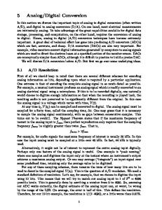
HARDWARE DESIGN TECHNIQUES 9.1 PASSIVE COMPONENTS Dielectric Absorption Dielectric absorption, which is also known as "soakage" and sometimes as "dielectric hysteresis"—is perhaps the least understood and potentially most damaging of various capacitor parasitic effects. Upon discharge, most capacitors are reluctant to give up all of their former charge, due to this memory consequence. Figure 9.2 illustrates this effect. On the left of the diagram, after being charged to the source potential of V volts at time to, the capacitor is shorted by the switch S1 at time t1, discharging it. At time t2, the capacitor is then open-circuited; a residual voltage slowly builds up across its terminals and reaches a nearly constant value. This error voltage is due to DA, and is shown in the right figure, a time/voltage representation of the charge/discharge/recovery sequence. Note that the recovered voltage error is proportional to both the original charging voltage V, as well as the rated DA for the capacitor in use. VO

S1 t0 V V

t1

C

V x DA

VO

t2

t t0

t1

t2

Figure 9.2: A Residual Open-Circuit Voltage After Charge/Discharge Characterizes Capacitor Dielectric Absorption Standard techniques for specifying or measuring dielectric absorption are few and far between. Measured results are usually expressed as the percentage of the original charging voltage that reappears across the capacitor. Typically, the capacitor is charged for a long period, then shorted for a shorter established time. The capacitor is then allowed to recover for a specified period, and the residual voltage is then measured (see Reference 8 for details). While this explanation describes the basic phenomenon, it is important to note that real-world capacitors vary quite widely in their susceptibility to this error, with their rated DA ranging from well below to above 1%, the exact number being a function of the dielectric material used. In practice, DA makes itself known in a variety of ways. Perhaps an integrator refuses to reset to zero, a voltage-to-frequency converter exhibits unexpected nonlinearity, or a sample-hold amplifier (SHA) exhibits varying errors. This last manifestation can be particularly damaging in a data-acquisition system, where adjacent channels may be at voltages which differ by nearly full scale, as shown below. Figure 9.3 illustrates the case of DA error in a simple SHA. On the left, switches S1 and S2 represent an input multiplexer and SHA switch, respectively. The multiplexer output voltage is VX, and the sampled voltage held on C is VY, which is buffered by the op amp for presentation to an ADC. As can be noted by the timing diagram on the right, a DA error voltage, ∈, appears in the hold mode, when the capacitor is effectively open circuit. 9.3

ANALOG-DIGITAL CONVERSION This voltage is proportional to the difference of voltages V1 and V2, which, if at opposite extremes of the dynamic range, exacerbates the error. As a practical matter, the best solution for good performance in terms of DA in a SHA is to use only the best capacitor.

V1

TO ADC S1

S2

V1

VY VX

VY

V2 V3

VN

∈ = (V1-V2) DA

V2 VX

C

OPEN S2 CLOSED

Figure 9.3: Dielectric Absorption Induces Errors in SHA Applications

The DA phenomenon is a characteristic of the dielectric material itself, although inferior manufacturing processes or electrode materials can also affect it. DA is specified as a percentage of the charging voltage. It can range from a low of 0.02% for Teflon, polystyrene, and polypropylene capacitors, up to a high of 10% or more for some electrolytics. For some time frames, the DA of polystyrene can be as low as 0.002%. Common high-K ceramics and polycarbonate capacitor types display typical DA on the order of 0.2%, it should be noted this corresponds to ½ LSB at only 8 bits! Silver mica, glass, and tantalum capacitors typically exhibit even larger DA, ranging from 1.0% to 5.0%, with those of polyester devices falling in the vicinity of 0.5%. As a rule, if the capacitor spec sheet doesn't specifically discuss DA within your time frame and voltage range, exercise caution! Another type with lower specified DA is likely a better choice. DA can produce long tails in the transient response of fast-settling circuits, such as those found in high-pass active filters or ac amplifiers. In some devices used for such applications, Figure 9.1's RDA-CDA model of DA can have a time constant of milliseconds. Much longer time constants are also quite usual. In fact, several paralleled RDA-CDA circuit sections with a wide range of time constants can model some devices. In fast-charge, fast-discharge applications, the behavior of the DA mechanism resembles "analog memory"; the capacitor in effect tries to remember its previous voltage. In some designs, you can compensate for the effects of DA if it is simple and easily characterized, and you are willing to do custom tweaking. In an integrator, for instance, the output signal can be fed back through a suitable compensation network, tailored to cancel the circuit equivalent of the DA by placing a negative impedance effectively in parallel. Such compensation has been shown to improve SH circuit performance by factors of 10 or more (Reference 6). 9.4

HARDWARE DESIGN TECHNIQUES 9.1 PASSIVE COMPONENTS Capacitor Parasitics and Dissipation Factor In Figure 9.1, a capacitor's leakage resistance, RP, the effective series resistance, RS, and effective series inductance, L, act as parasitic elements, which can degrade an external circuit's performance. The effects of these elements are often lumped together and defined as a dissipation factor, or DF. A capacitor's leakage is the small current that flows through the dielectric when a voltage is applied. Although modeled as a simple insulation resistance (RP) in parallel with the capacitor, the leakage actually is nonlinear with voltage. Manufacturers often specify leakage as a megohm-microfarad product, which describes the dielectric's self-discharge time constant, in seconds. It ranges from a low of 1 second or less for high-leakage capacitors, such as electrolytic devices, to the 100s of seconds for ceramic capacitors. Glass devices exhibit self-discharge time-constants of 1,000 or more; but the best leakage performance is shown by Teflon and the film devices (polystyrene, polypropylene), with time constants exceeding 1,000,000 megohm-microfarads. For such a device, external leakage paths—created by surface contamination of the device's case or in the associated wiring or physical assembly—can overshadow the internal dielectric-related leakage. Effective series inductance, ESL (Figure 9.1, again) arises from the inductance of the capacitor leads and plates, which, particularly at the higher frequencies, can turn a capacitor's normally capacitive reactance into an inductive reactance. Its magnitude strongly depends on construction details within the capacitor. Tubular wrapped-foil devices display significantly more lead inductance than molded radial-lead configurations. Multilayer ceramic (MLC) and film-type devices typically exhibit the lowest series inductance, while ordinary tantalum and aluminum electrolytics typically exhibit the highest. Consequently, standard electrolytic types, if used alone, usually prove insufficient for high-speed local bypassing applications. Note however that there also are more specialized aluminum and tantalum electrolytics available, which may be suitable for higher speed uses, however, localized bypassing is still recommended. These are the types generally designed for use in switch-mode power supplies, which are covered more completely in a following section. Manufacturers of capacitors often specify effective series impedance by means of impedance-versus-frequency plots. Not surprisingly, these curves show graphically a predominantly capacitive reactance at low frequencies, with rising impedance at higher frequencies because of the effect of series inductance. Effective series resistance, ESR (resistor RS of Figure 9.1), is made up of the resistance of the leads and plates. As noted, many manufacturers lump the effects of ESR, ESL, and leakage into a single parameter called dissipation factor, or DF. Dissipation factor measures the basic inefficiency of the capacitor. Manufacturers define it as the ratio of the energy lost to energy stored per cycle by the capacitor. The ratio of ESR to total capacitive reactance—at a specified frequency—approximates the dissipation factor, which turns out to be equivalent to the reciprocal of the figure of merit, Q. Stated as an approximation, Q ≈ 1/DF (with DF in numeric terms). For example, a DF of 0.1% is equivalent to a fraction of 0.001; thus the inverse in terms of Q would be 1000.

9.5

ANALOG-DIGITAL CONVERSION Dissipation factor often varies as a function of both temperature and frequency. Capacitors with mica and glass dielectrics generally have DF values from 0.03% to 1.0%. For ceramic devices, DF ranges from a low of 0.1 % to as high as 2.5% at room temperature. And electrolytics usually exceed even this level. The film capacitors are the best as a group, with DFs of less than 0.1 %. Stable-dielectric ceramics, notably the NP0 (also called COG) types, have DF specs comparable to films (more below). Tolerance, Temperature, and Other Effects In general, precision capacitors are expensive and—even then—not necessarily easy to buy. In fact, choice of capacitance is limited both by the range of available values, and also by tolerances. In terms of size, the better performing capacitors in the film families tend to be limited in practical terms to 10 µF or less (for dual reasons of size and expense). In terms of low value tolerance, ±1% is possible for NP0 ceramic and some film devices, but with possibly unacceptable delivery times. Many film capacitors can be made available with tolerances of less than ±1%, but on a special order basis only. Most capacitors are sensitive to temperature variations. DF, DA, and capacitance value are all functions of temperature. For some capacitors, these parameters vary approximately linearly with temperature, in others they vary quite nonlinearly. Although it is usually not important for SHA applications, an excessively large temperature coefficient (TC, measured in ppm/°C) can prove harmful to the performance of precision integrators, voltage-to-frequency converters, and oscillators. NP0 ceramic capacitors, with TCs as low as 30 ppm/°C, are the best for stability, with polystyrene and polypropylene next best, with TCs in the 100-200 ppm/°C range. On the other hand, when capacitance stability is important, one should stay away from types with TCs of more than a few hundred ppm/°C, or in fact any TC which is nonlinear. A capacitor's maximum working temperature should also be considered, in light of the expected environment. Polystyrene capacitors, for instance, melt near 85°C, compared to Teflon's ability to survive temperatures up to 200°C. Sensitivity of capacitance and DA to applied voltage, expressed as voltage coefficient, can also hurt capacitor performance within a circuit application. Although capacitor manufacturers don't always clearly specify voltage coefficients, the user should always consider the possible effects of such factors. For instance, when maximum voltages are applied, some high-K ceramic devices can experience a decrease in capacitance of 50% or more. This is an inherent distortion producer, making such types unsuitable for signal path filtering, for example, and better suited for supply bypassing. Interestingly, NP0 ceramics, the stable dielectric subset from the wide range of available ceramics, do offer good performance with respect to voltage coefficient. Similarly, the capacitance and dissipation factor of many types vary significantly with frequency, mainly as a result of a variation in dielectric constant. In this regard, the better dielectrics are polystyrene, polypropylene, and Teflon.

9.6

HARDWARE DESIGN TECHNIQUES 9.1 PASSIVE COMPONENTS Assemble Critical Components Last The designer's worries don't end with the design process. Some common printed circuit assembly techniques can prove ruinous to even the best designs. For instance, some commonly used cleaning solvents can infiltrate certain electrolytic capacitors—those with rubber end caps are particularly susceptible. Even worse, some of the film capacitors, polystyrene in particular, actually melt when contacted by some solvents. Rough handling of the leads can damage still other capacitors, creating random or even intermittent circuit problems. Etched-foil types are particularly delicate in this regard. To avoid these difficulties it may be advisable to mount especially critical components as the last step in the board assembly process—if possible. Table 9.1 summarizes selection criteria for various capacitor types, arranged roughly in order of decreasing DA performance. In a selection process, the general information of this table should be supplemented by consultation of current vendor's catalog information (see References at end of section). Designers should also consider the natural failure mechanisms of capacitors. Metallized film devices, for instance, often self-heal. They initially fail due to conductive bridges that develop through small perforations in the dielectric film. But, the resulting fault currents can generate sufficient heat to destroy the bridge, thus returning the capacitor to normal operation (at a slightly lower capacitance). Of course, applications in high-impedance circuits may not develop sufficient current to clear the bridge, so the designer must be wary here. Tantalum capacitors also exhibit a degree of self-healing, but—unlike film capacitors— the phenomenon depends on the temperature at the fault location rising slowly. Therefore, tantalum capacitors self-heal best in high impedance circuits which limit the surge in current through the capacitor's defect. Use caution therefore, when specifying tantalums for high-current applications. Electrolytic capacitor life often depends on the rate at which capacitor fluids seep through end caps. Epoxy end seals perform better than rubber seals, but an epoxy sealed capacitor can explode under severe reverse-voltage or overvoltage conditions. Finally, all polarized capacitors must be protected from exposure to voltages outside their specifications.

9.7

ANALOG-DIGITAL CONVERSION

Table 9.1 Capacitor Comparison Chart TYPE

TYPICAL DA

ADVANTAGES

DISADVANTAGES

Polystyrene

0.001% to 0.02%

Inexpensive Low DA Good stability (~120ppm/°C)

Damaged by temperature > +85°C Large High inductance Vendors limited

Polypropylene

0.001% to 0.02%

Inexpensive Low DA Stable (~200ppm/°C) Wide range of values

Damaged by temperature > +105°C Large High inductance

Teflon

0.003% to 0.02%

Low DA available Good stability Operational above +125 °C Wide range of values

Expensive Large High inductance

Polycarbonate

0.1%

Good stability Low cost Wide temperature range Wide range of values

Large DA limits to 8-bit applications High inductance

Polyester

0.3% to 0.5%

Moderate stability Low cost Wide temperature range Low inductance (stacked film)

Large DA limits to 8-bit applications High inductance (conventional)

NP0 Ceramic

0.2%

Low inductance (chip) Wide range of values

Poor stability Poor DA High voltage coefficient

Mica

>0.003%

Low loss at HF Low inductance Good stability 1% values available

Quite large Low maximum values (≤ 10nF) Expensive

Aluminum Electrolytic

Very high

Large values High currents High voltages Small size

High leakage Usually polarized Poor stability, accuracy Inductive

Tantalum Electrolytic

Very high

Small size Large values Medium inductance

High leakage Usually polarized Expensive Poor stability, accuracy

9.8

HARDWARE DESIGN TECHNIQUES 9.1 PASSIVE COMPONENTS

Resistors and Potentiometers Designers have a broad range of resistor technologies to choose from, including carbon composition, carbon film, bulk metal, metal film, and both inductive and non-inductive wire-wound types. As perhaps the most basic—and presumably most trouble-free—of components, resistors are often overlooked as error sources in high performance circuits. Yet, an improperly selected resistor can subvert the accuracy of a 12-bit design by developing errors well in excess of 122 ppm (½ LSB). When did you last read a resistor data sheet? You'd be surprised what can be learned from an informed review of data.

+

_

G=1+

R1 = 100 R2

R1 = 9.9kΩ, 1/4 W TC = +25ppm/°c R2 = 100Ω, 1/4 W TC = +50ppm/°c

Temperature change of 10°C causes gain change of 250ppm This is 1LSB in a 12-bit system and a disaster in a 16-bit system

Figure 9.4: Mismatched Resistor TCs Can Induce Temperature-Related Gain Errors Consider the simple circuit of Figure 9.4, showing a non-inverting op amp where the 100× gain is set by R1 and R2. The TCs of these two resistors are a somewhat obvious source of error. Assume the op amp gain errors to be negligible, and that the resistors are perfectly matched to a 99/1 ratio at +25ºC. If, as noted, the resistor TCs differ by only 25 ppm/ºC, the gain of the amplifier changes by 250 ppm for a 10ºC temperature change. This is about a 1 LSB error in a 12-bit system, and a major disaster in a 16-bit system. Temperature changes, however, can limit the accuracy of the Figure 9.4 amplifier in several ways. In this circuit (as well as many op amp circuits with component-ratio defined gains), the absolute TC of the resistors is less important—as long as they track one another in ratio. But even so, some resistor types simply aren't suitable for precise work. For example, carbon composition units—with TCs of approximately 1,500 ppm/°C, won't work. Even if the TCs could be matched to an unlikely 1%, the resulting 15-ppm/°C differential still proves inadequate—an 8°C shift creates a 120-ppm error. Many manufacturers offer metal film and bulk metal resistors, with absolute TCs ranging between ±1 and ±100 ppm/°C. Beware, though; TCs can vary a great deal, particularly 9.9

ANALOG-DIGITAL CONVERSION among discrete resistors from different batches. To avoid this problem, more expensive matched resistor pairs are offered by some manufacturers, with temperature coefficients that track one another to within 2 to 10 ppm/°C. Low-priced thin-film networks have good relative performance and are widely used. +100mV

+

G=1+

R1 = 100 R2

+10V _

R1 = 9.9kΩ, 1/4 W TC = +25ppm/°c

Assume TC of R1 = TC of R2

R2 = 100Ω, 1/4 W TC = +25ppm/°c

R1, R2 Thermal Resistance = 125°c / W Temperature of R1 will rise by 1.24°C, PD = 9.9mW Temperature rise of R2 is negligible, PD = 0.1mW Gain is altered by 31ppm, or 1/2 LSB @ 14-bits

Figure 9.5: Uneven Power Dissipation Between Resistors With Identical TCs Can Also Introduce Temperature-Related Gain Errors Suppose, as shown in Figure 9.5, R1 and R2 are ¼W resistors with identical 25-ppm/ºC TCs. Even when the TCs are identical, there can still be significant errors! When the signal input is zero, the resistors dissipate no heat. But, if it is 100 mV, there is 9.9 V across R1, which then dissipates 9.9 mW. It will experience a temperature rise of 1.24ºC (due to a 125ºC/W, ¼W resistor thermal resistance). This 1.24ºC rise causes a resistance change of 31 ppm, and thus a corresponding gain change. But R2, with only 100 mV across it, is only heated a negligible 0.0125ºC. The resulting 31-ppm net gain error represents a fullscale error of ½ LSB at 14-bits, and is a disaster for a 16-bit system. Even worse, the effects of this resistor self-heating also create easily calculable nonlinearity errors. In the Figure 9.5 example, with ½ the voltage input, the resulting self-heating error is only 15 ppm. In other words, the stage gain is not constant at ½ and full-scale (nor is it so at other points), as long as uneven temperature shifts exist between the gain-determining resistors. This is by no means a worst-case example; physically smaller resistors would give worse results, due to higher associated thermal resistance. These, and similar errors, are avoided by selecting critical resistors that are accurately matched for both value and TC, are well derated for power, and have tight thermal coupling between those resistors were matching is important. This is best achieved by using a resistor network on a single substrate—such a network may either be within an IC, or it may be a separately packaged thin-film resistor network.

9.10

HARDWARE DESIGN TECHNIQUES 9.1 PASSIVE COMPONENTS When the circuit resistances are very low (≤10 Ω), interconnection stability also becomes important. For example, while often overlooked as an error, the resistance TC of typical copper wire or printed circuit traces can add errors. The TC of copper is typically ~3,900 ppm/°C. Thus a precision 10-Ω, 10-ppm/°C wirewound resistor with 0.1 Ω of copper interconnect effectively becomes a 10.1-Ω resistor with a TC of nearly 50 ppm/°C. One final consideration applies mainly to designs that see widely varying ambient temperatures: a phenomenon known as temperature retrace describes the change in resistance which occurs after a specified number of cycles of exposure to low and high ambients with constant internal dissipation. Temperature retrace can exceed 10 ppm/°C, even for some of the better thin-film components. In summary, to design resistance-based circuits for minimum temperature-related errors, consider the points noted in Figure 9.6 (along with their cost). Closely match resistance TCs. Use resistors with low absolute TCs. Use resistors with low thermal resistance (higher power ratings, larger cases). Tightly couple matched resistors thermally (use standard commonsubstrate networks). For large ratios consider using stepped attenuators.

Figure 9.6: A Number of Points are Important Towards Minimizing Temperature-Related Errors in Resistors Resistor Parasitics Resistors can exhibit significant levels of parasitic inductance or capacitance, especially at high frequencies. Manufacturers often specify these parasitic effects as a reactance error, in % or ppm, based on the ratio of the difference between the impedance magnitude and the dc resistance, to the resistance, at one or more frequencies. Wirewound resistors are especially susceptible to difficulties. Although resistor manufacturers offer wirewound components in either normal or noninductively wound form, even noninductively wound resistors create headaches for designers. These resistors still appear slightly inductive (of the order of 20 µH) for values below 10 kΩ. Above 10 kΩ the same style resistors actually exhibit 5 pF of shunt capacitance. These parasitic effects can raise havoc in dynamic circuit applications. Of particular concern are applications using wirewound resistors with values greater than 10 kΩ. Here it isn't uncommon to see peaking, or even oscillation. These effects become more evident at low-kHz frequency ranges.

9.11

ANALOG-DIGITAL CONVERSION Even in low-frequency circuit applications, parasitic effects in wirewound resistors can create difficulties. Exponential settling to 1 ppm may take 20 time constants or more. The parasitic effects associated with wirewound resistors can significantly increase net circuit settling time to beyond the length of the basic time constants. Unacceptable amounts of parasitic reactance are often found even in resistors that aren't wirewound. For instance, some metal-film types have significant interlead capacitance, which shows up at high frequencies. In contrast, when considering this end-to-end capacitance, carbon resistors do the best at high frequencies. Thermoelectric Effects Another more subtle problem with resistors is the thermocouple effect, also sometimes referred to as thermal EMF. Wherever there is a junction between two different metallic conductors, a thermoelectric voltage results. The thermocouple effect is widely used to measure temperature. However, in any low level precision op amp circuit it is also a potential source of inaccuracy, since wherever two different conductors meet, a thermocouple is formed (whether we like it or not). In fact, in many cases, it can easily produce the dominant error within an otherwise precision circuit design. Parasitic thermocouples will cause errors when and if the various junctions forming the parasitic thermocouples are at different temperatures. With two junctions present on each side of the signal being processed within a circuit, by definition we have formed at least one thermocouple pair. If the two junctions of this thermocouple pair are at different temperatures, there will be a net temperature dependent error voltage produced. Conversely, if the two junctions of a parasitic thermocouple pair are kept at an identical temperature, then the net error produced will be zero, as the voltages of the two thermocouples effectively will be canceled. This is a critically important point, since in practice we cannot avoid connecting dissimilar metals together to build an electronic circuit. But, what we can do is carefully control temperature differentials across the circuit, so such that the undesired thermocouple errors cancel one another. The effect of such parasitics is very hard to avoid. To understand this, consider a case of making connections with copper wire only. In this case, even a junction formed by different copper wire alloys can have a thermoelectric voltage which is a small fraction of 1 µV/ºC! And, taking things a step further, even such apparently benign components as resistors contain parasitic thermocouples, with potentially even stronger effects. For example, consider the resistor model shown in Figure 9.7. The two connections between the resistor material and the leads form thermocouple junctions, T1 and T2. This thermocouple EMF can be as high as 400 µV/ºC for some carbon composition resistors, and as low as 0.05 µV/ºC for specially constructed resistors (see Reference 15). Ordinary metal film resistors (RN-types) are typically about 20 µV/ºC.

9.12

HARDWARE DESIGN TECHNIQUES 9.1 PASSIVE COMPONENTS +

+

RESISTOR MATERIAL

T1

T2 +

RESISTOR LEADS TYPICAL RESISTOR THERMOCOUPLE EMFs CARBON COMPOSITION

≈ 400 µV/ °C

METAL FILM

≈ 20 µV/ °C

EVENOHM OR MANGANIN WIREWOUND

≈ 2 µV/ °C

RCD Components HP-Series

≈ 0.05 µV/ °C

Figure 9.7: Every Resistor Contains Two Thermocouples, Formed Between the Leads and Resistance Element Note that these thermocouple effects are relatively unimportant for ac signals. Even for dc-only signals, they will nicely cancel one another, if, as noted above, the entire resistor is at a uniform temperature. However, if there is significant power dissipation in a resistor, or if its orientation with respect to a heat source is non-symmetrical, this can cause one of its ends to be warmer than the other, causing a net thermocouple error voltage. Using ordinary metal film resistors, an end-to-end temperature differential of 1ºC causes a thermocouple voltage of about 20 µV. This error level is quite significant compared to the offset voltage drift of a precision op amp like the OP177, and extremely significant when compared to chopper-stabilized op amps, with their drifts of 1 LSB of Error due to Drop In PCB Conductor So, when dealing with precision circuits, the point is made that even simple design items such as PCB trace resistance cannot be dealt with casually. There are various solutions that can address this issue, such as wider traces (which may take up excessive space), the use of heavier copper (which may be too expensive), or simply choosing a high impedance converter. But, the most important thing is to think it all through, avoiding any tendency to overlook items appearing innocuous on the surface.

Voltage Drop in Signal Leads—"Kelvin" Feedback The gain error resulting from resistive voltage drop in PCB signal leads is important only with high precision and/or at high resolutions (the Figure 9.17 example), or where large signal currents flow. Where load impedance is constant and resistive, adjusting overall system gain can compensate for the error. In other circumstances, it may often be removed by the use of "Kelvin" or "voltage sensing" feedback, as shown in Figure 9.18. FEEDBACK "SENSE" LEAD S

SIGNAL SOURCE

HIGH RESISTANCE SIGNAL LEAD

F

ADC with low RIN

Assume ground path resistance negligible

Figure 9.18: Use of a Sense Connection Moves Accuracy to the Load Point

9.27

ANALOG-DIGITAL CONVERSION In this modification to the case of Figure 9.17, a long resistive PCB trace is still used to drive the input of a high resolution ADC, with low input impedance. In this case however, the voltage drop in the signal lead does not give rise to an error, as feedback is taken directly from the input pin of the ADC, and returned to the driving source. This scheme allows full accuracy to be achieved in the signal presented to the ADC, despite any voltage drop across the signal trace. The use of separate force (F) and sense (S) connections at the load removes any errors resulting from voltage drops in the force lead, but, of course, may only be used in systems where there is negative feedback. It is also impossible to use such an arrangement to drive two or more loads with equal accuracy, since feedback may only be taken from one point. Also, in this much-simplified system, errors in the common lead source/load path are ignored, the assumption being that ground path voltages are negligible. In many systems this may not necessarily be the case, and additional steps may be needed, as noted below.

Signal Return Currents Kirchoff's Law tells us that at any point in a circuit the algebraic sum of the currents is zero. This tells us that all currents flow in circles and, particularly, that the return current must always be considered when analyzing a circuit, as is illustrated in Figure 9.19 (see References 7 and 8). SIGNAL SOURCE

I

LOAD

RL

G1

GROUND RETURN CURRENT

I

I

G2

AT ANY POINT IN A CIRCUIT THE ALGEBRAIC SUM OF THE CURRENTS IS ZERO OR WHAT GOES OUT MUST COME BACK WHICH LEADS TO THE CONCLUSION THAT ALL VOLTAGES ARE DIFFERENTIAL (EVEN IF THEY’RE GROUNDED)

Figure 9.19: Kirchoff’s Law Helps in Analyzing Voltage Drops Around a Complete Source/Load Coupled Circuit In dealing with grounding issues, common human tendencies provide some insight into how the correct thinking about the circuit can be helpful towards analysis. Most engineers readily consider the ground return current, "I", when they are considering a fully differential circuit. However, when considering the more usual circuit case, where a single-ended signal is referred to "ground", it is common to assume that all the points on the circuit diagram 9.28

HARDWARE DESIGN TECHNIQUES 9.2 PC BOARD DESIGN ISSUES where ground symbols are found are at the same potential. Unfortunately, this happy circumstance just ain't necessarily so! This overly optimistic approach is illustrated in Figure 9.20, where, if it really should exist, "infinite ground conductivity" would lead to zero ground voltage difference between source ground G1 and load ground G2. Unfortunately this approach isn’t a wise practice, and when dealing with high precision circuits, it can lead to disasters. SIGNAL

ADC

SIGNAL SOURCE

INFINITE GROUND CONDUCTIVITY

G1

G2

→ ZERO VOLTAGE DIFFERENTIAL BETWEEN G1 & G2

Figure 9.20: Unlike This Optimistic Diagram, it is Unrealistic to Assume Infinite Conductivity Between Source/Load Grounds in a Real-World System A more realistic approach to ground conductor integrity includes analysis of the impedance(s) involved, and careful attention to minimizing spurious noise voltages. A more realistic model of a ground system is shown in Figure 9.21. The signal return current flows in the complex impedance existing between ground points G1 and G2 as shown, giving rise to a voltage drop ∆V in this path. But it is important to note that additional external currents, such as IEXT, may also flow in this same path. It is critical to understand that such currents may generate uncorrelated noise voltages between G1 and G2 (dependent upon the current magnitude and relative ground impedance). SIGNAL

LOAD

SIGNAL SOURCE

ISIG ∆V = VOLTAGE DIFFERENTIAL DUE TO SIGNAL CURRENT AND/OR EXTERNAL CURRENT FLOWING IN GROUND IMPEDANCE

G1

G2

IEXT

Figure 9.21: A More Realistic Source-to-Load Grounding System View Includes Consideration of the Impedance Between G1-G2, Plus the Effect of Any NonSignal-Related Currents 9.29

ANALOG-DIGITAL CONVERSION Some portion of these undesired voltages may end up being seen at the signal's load end, and they can have the potential to corrupt the signal being transmitted.

Grounding in Mixed Analog/Digital Systems Walt Kester, James Bryant, Mike Byrne Today's signal processing systems generally require mixed-signal devices such as analogto-digital converters (ADCs) and digital-to-analog converters (DACs) as well as fast digital signal processors (DSPs). Requirements for processing analog signals having wide dynamic ranges increases the importance of high performance ADCs and DACs. Maintaining wide dynamic range with low noise in hostile digital environments is dependent upon using good high-speed circuit design techniques including proper signal routing, decoupling, and grounding. In the past, "high precision, low-speed" circuits have generally been viewed differently than so-called "high-speed" circuits. With respect to ADCs and DACs, the sampling (or update) frequency has generally been used as the distinguishing speed criteria. However, the following two examples show that in practice, most of today's signal processing ICs are really "high-speed," and must therefore be treated as such in order to maintain high performance. This is certainly true of DSPs, and also true of ADCs and DACs. All sampling ADCs (ADCs with an internal sample-and-hold circuit) suitable for signal processing applications operate with relatively high speed clocks with fast rise and fall times (generally a few nanoseconds) and must be treated as high speed devices, even though throughput rates may appear low. For example, a medium-speed 12-bit successive approximation (SAR) ADC may operate on a 10-MHz internal clock, while the sampling rate is only 500 kSPS. Sigma-delta (Σ-∆) ADCs also require high speed clocks because of their high oversampling ratios. Even high resolution, so-called "low frequency" Σ-∆ industrial measurement ADCs (having throughputs of 10 Hz to 7.5 kHz) operate on 5-MHz or higher clocks and offer resolution to 24-bits (for example, the Analog Devices AD77xxseries). To further complicate the issue, mixed-signal ICs have both analog and digital ports, and because of this, much confusion has resulted with respect to proper grounding techniques. In addition, some mixed-signal ICs have relatively low digital currents, while others have high digital currents. In many cases, these two types must be treated differently with respect to optimum grounding. Digital and analog design engineers tend to view mixed-signal devices from different perspectives, and the purpose of this section is to develop a general grounding philosophy that will work for most mixed signal devices, without having to know the specific details of their internal circuits. Ground and Power Planes The importance of maintaining a low impedance large area ground plane is critical to all analog circuits today. The ground plane not only acts as a low impedance return path for 9.30

HARDWARE DESIGN TECHNIQUES 9.2 PC BOARD DESIGN ISSUES decoupling high frequency currents (caused by fast digital logic) but also minimizes EMI/RFI emissions. Because of the shielding action of the ground plane, the circuit's susceptibility to external EMI/RFI is also reduced. Ground planes also allow the transmission of high speed digital or analog signals using transmission line techniques (microstrip or stripline) where controlled impedances are required. The use of "buss wire" is totally unacceptable as a "ground" because of its impedance at the equivalent frequency of most logic transitions. For instance, #22 gauge wire has about 20 nH/inch inductance. A transient current having a slew rate of 10 mA/ns created by a logic signal would develop an unwanted voltage drop of 200 mV at this frequency flowing through 1 inch of this wire: ∆v = L

∆i 10 mA = 20 nH × = 200 mV. ∆t ns

Eq. 9.1

For a signal having a 2-V peak-to-peak range, this translates into an error of about 200 mV, or 10% (approximate 3.5-bit accuracy). Even in all-digital circuits, this error would result in considerable degradation of logic noise margins. Figure 9.22 shows an illustration of a situation where the digital return current modulates the analog return current (top figure). The ground return wire inductance and resistance is shared between the analog and digital circuits, and this is what causes the interaction and resulting error. A possible solution is to make the digital return current path flow directly to the GND REF as shown in the bottom figure. This is the fundamental concept of a "star," or single-point ground system. Implementing the true single-point ground in a system which contains multiple high frequency return paths is difficult because the physical length of the individual return current wires will introduce parasitic resistance and inductance which can make obtaining a low impedance high frequency ground difficult. In practice, the current returns must consist of large area ground planes for low impedance to high frequency currents. Without a low-impedance ground plane, it is therefore almost impossible to avoid these shared impedances, especially at high frequencies. All integrated circuit ground pins should be soldered directly to the low-impedance ground plane to minimize series inductance and resistance. The use of traditional IC sockets is not recommended with high-speed devices. The extra inductance and capacitance of even "low profile" sockets may corrupt the device performance by introducing unwanted shared paths. If sockets must be used with DIP packages, as in prototyping, individual "pin sockets" or "cage jacks" may be acceptable. Both capped and uncapped versions of these pin sockets are available (AMP part numbers 5-330808-3, and 5-330808-6). They have spring-loaded gold contacts which make good electrical and mechanical connection to the IC pins. Multiple insertions, however, may degrade their performance.

9.31

ANALOG-DIGITAL CONVERSION

ID IA + VD

INCORRECT

+ VA

ANALOG CIRCUITS

VIN

GND REF

I A + ID

DIGITAL CIRCUITS

ID

ID IA + VD

+ VA

GND REF

VIN

CORRECT ANALOG CIRCUITS

DIGITAL CIRCUITS

IA ID

Figure 9.22: Digital Currents Flowing in Analog Return Path Create Error Voltages Power supply pins should be decoupled directly to the ground plane using low inductance ceramic surface mount capacitors. If through-hole mounted ceramic capacitors must be used, their leads should be less than 1 mm. The ceramic capacitors should be located as close as possible to the IC power pins. Ferrite beads may be also required for additional decoupling. Double-Sided vs. Multilayer Printed Circuit Boards Each PCB in the system should have at least one complete layer dedicated to the ground plane. Ideally, a double-sided board should have one side completely dedicated to ground and the other side for interconnections. In practice, this is not possible, since some of the ground plane will certainly have to be removed to allow for signal and power crossovers, vias, and through-holes. Nevertheless, as much area as possible should be preserved, and at least 75% should remain. After completing an initial layout, the ground layer should be checked carefully to make sure there are no isolated ground "islands," because IC ground pins located in a ground "island" have no current return path to the ground plane. Also, the ground plane should be checked for "skinny" connections between adjacent large areas which may significantly reduce the effectiveness of the ground plane. Needless to say, auto-routing board layout techniques will generally lead to a layout disaster on a mixed-signal board, so manual intervention is highly recommended. Systems that are densely packed with surface mount ICs will have a large number of interconnections; therefore multilayer boards are mandatory. This allows at least one complete layer to be dedicated to ground. A simple 4-layer board would have internal ground and power plane layers with the outer two layers used for interconnections 9.32

HARDWARE DESIGN TECHNIQUES 9.2 PC BOARD DESIGN ISSUES between the surface mount components. Placing the power and ground planes adjacent to each other provides additional inter-plane capacitance which helps high frequency decoupling of the power supply. In most systems, 4-layers are not enough, and additional layers are required for routing signals as well as power. Figure 9.23 summarizes the key issues relating to ground planes. Use Large Area Ground (and Power) Planes for Low Impedance Current Return Paths (Must Use at Least a Double-Sided Board!) Double-Sided Boards: Avoid High-Density Interconnection Crossovers and Vias Which Reduce Ground Plane Area Keep > 75% Board Area on One Side for Ground Plane Multilayer Boards: Mandatory for Dense Systems Dedicate at Least One Layer for the Ground Plane Dedicate at Least One Layer for the Power Plane Use at Least 30% to 40% of PCB Connector Pins for Ground Continue the Ground Plane on the Backplane Motherboard to Power Supply Return

Figure 9.23: Ground Planes Are Mandatory! Multicard Mixed-Signal Systems The best way of minimizing ground impedance in a multicard system is to use a "motherboard" PCB as a backplane for interconnections between cards, thus providing a continuous ground plane to the backplane. The PCB connector should have at least 3040% of its pins devoted to ground, and these pins should be connected to the ground plane on the backplane mother card. To complete the overall system grounding scheme there are two possibilities: 1. The backplane ground plane can be connected to chassis ground at numerous points, thereby diffusing the various ground current return paths. This is commonly referred to as a "multipoint" grounding system and is shown in Figure 9.24. 2. The ground plane can be connected to a single system "star ground" point (generally at the power supply). The first approach is most often used in all-digital systems, but can be used in mixedsignal systems provided the ground currents due to digital circuits are sufficiently low and diffused over a large area. The low ground impedance is maintained all the way through the PC boards, the backplane, and ultimately the chassis. However, it is critical that good electrical contact be made where the grounds are connected to the sheet metal chassis. This requires self-tapping sheet metal screws or "biting" washers. Special care must be taken where anodized aluminum is used for the chassis material, since its surface acts as an insulator. 9.33

ANALOG-DIGITAL CONVERSION

VA

PCB

VD

GROUND PLANE

VA

PCB

VD

GROUND PLANE

BACKPLANE

GROUND PLANE

CHASSIS GROUND

POWER SUPPLIES

VA VD

Figure 9.24: Multipoint Ground Concept The second approach ("star ground") is often used in high speed mixed-signal systems having separate analog and digital ground systems and warrants further discussion. Separating Analog and Digital Grounds In mixed-signal systems with large amounts of digital circuitry, it is highly desirable to physically separate sensitive analog components from noisy digital components. It may also be beneficial to use separate ground planes for the analog and the digital circuitry. These planes should not overlap in order to minimize capacitive coupling between the two. The separate analog and digital ground planes are continued on the backplane using either motherboard ground planes or "ground screens" which are made up of a series of wired interconnections between the connector ground pins. The arrangement shown in Figure 9.25 illustrates that the two planes are kept separate all the way back to a common system "star" ground, generally located at the power supplies. The connections between the ground planes, the power supplies, and the "star" should be made up of multiple bus bars or wide copper braids for minimum resistance and inductance. The back-to-back Schottky diodes on each PCB are inserted to prevent accidental dc voltage from developing between the two ground systems when cards are plugged and unplugged. This voltage should be kept less than 300 mV to prevent damage to ICs which have connections to both the analog and digital ground planes. Schottky diodes are preferable because of their low capacitance and low forward voltage drop. The low capacitance prevents ac coupling between the analog and digital ground planes. Schottky diodes begin to conduct at about 300 mV, and several parallel diodes in parallel may be required if high currents are expected. In some cases, ferrite beads can be used instead of Schottky diodes, however they introduce dc ground loops which can be troublesome in precision systems. 9.34

HARDWARE DESIGN TECHNIQUES 9.2 PC BOARD DESIGN ISSUES

VA ANALOG GROUND PLANE

PCB

VD

VA

DIGITAL GROUND PLANE

ANALOG GROUND PLANE

D

A

PCB

VD DIGITAL GROUND PLANE

D

A

DIGITAL GROUND PLANE

BACKPLANE ANALOG GROUND PLANE

SYSTEM STAR GROUND

POWER SUPPLIES

VA VD

Figure 9.25: Separating Analog and Digital Ground Planes It is mandatory that the impedance of the ground planes be kept as low as possible, all the way back to the system star ground. DC or ac voltages of more than 300 mV between the two ground planes can not only damage ICs but cause false triggering of logic gates and possible latchup. Grounding and Decoupling Mixed-Signal ICs with Low Digital Currents Sensitive analog components such as amplifiers and voltage references are always referenced and decoupled to the analog ground plane. The ADCs and DACs (and other mixed-signal ICs) with low digital currents should generally be treated as analog components and also grounded and decoupled to the analog ground plane. At first glance, this may seem somewhat contradictory, since a converter has an analog and digital interface and usually has pins designated as analog ground (AGND) and digital ground (DGND). The diagram shown in Figure 9.26 will help to explain this seeming dilemma. Inside an IC that has both analog and digital circuits, such as an ADC or a DAC, the grounds are usually kept separate to avoid coupling digital signals into the analog circuits. Figure 9.26 shows a simple model of a converter. There is nothing the IC designer can do about the wirebond inductance and resistance associated with connecting the bond pads on the chip to the package pins except to realize it's there. The rapidly changing digital currents produce a voltage at point B which will inevitably couple into point A of the analog circuits through the stray capacitance, CSTRAY. In addition, there is approximately 0.2-pF unavoidable stray capacitance between every pin of the IC package! It's the IC designer's job to make the chip work in spite of this. However, in order to prevent further coupling, the AGND and DGND pins should be joined together 9.35

ANALOG-DIGITAL CONVERSION externally to the analog ground plane with minimum lead lengths. Any extra impedance in the DGND connection will cause more digital noise to be developed at point B; it will, in turn, couple more digital noise into the analog circuit through the stray capacitance. Note that connecting DGND to the digital ground plane applies VNOISE across the AGND and DGND pins and invites disaster! VA

VD

FERRITE BEAD

A

LP

LP

CSTRAY

RP

AIN/ OUT

ANALOG CIRCUITS

LP

R

B CSTRAY IA

ID

AGND A

SEE TEXT

RP

DIGITAL CIRCUITS DATA

A RP

D

VD

VA

SHORT CONNECTIONS

BUFFER GATE OR REGISTER

DATA BUS

CIN ≈ 10pF

RP LP

DGND A

A = ANALOG GROUND PLANE

VNOISE

D

D = DIGITAL GROUND PLANE

Figure 9.26: Proper Grounding of Mixed-signal ICs With Low Internal Digital Currents The name "DGND" on an IC tells us that this pin connects to the digital ground of the IC. This does not imply that this pin must be connected to the digital ground of the system. It is true that this arrangement may inject a small amount of digital noise onto the analog ground plane. These currents should be quite small, and can be minimized by ensuring that the converter output does not drive a large fanout (they normally can't, by design). Minimizing the fanout on the converter's digital port will also keep the converter logic transitions relatively free from ringing and minimize digital switching currents, and thereby reducing any potential coupling into the analog port of the converter. The logic supply pin (VD) can be further isolated from the analog supply by the insertion of a small lossy ferrite bead as shown in Figure 9.26. The internal transient digital currents of the converter will flow in the small loop from VD through the decoupling capacitor and to DGND (this path is shown with a heavy line on the diagram). The transient digital currents will therefore not appear on the external analog ground plane, but are confined to the loop. The VD pin decoupling capacitor should be mounted as close to the converter as possible to minimize parasitic inductance. These decoupling capacitors should be low inductance ceramic types, typically between 0.01 µF and 0.1 µF.

9.36

HARDWARE DESIGN TECHNIQUES 9.2 PC BOARD DESIGN ISSUES Treat the ADC Digital Outputs with Care It is always a good idea (as shown in Figure 9.26) to place a buffer register adjacent to the converter to isolate the converter's digital lines from noise on the data bus. The register also serves to minimize loading on the digital outputs of the converter and acts as a Faraday shield between the digital outputs and the data bus. Even though many converters have three-state outputs/inputs, this isolation register still represents good design practice. In some cases it may be desirable to add an additional buffer register on the analog ground plane next to the converter output to provide greater isolation. The series resistors (labeled "R" in Figure 9.26) between the ADC output and the buffer register input help to minimize the digital transient currents which may affect converter performance. The resistors isolate the digital output drivers from the capacitance of the buffer register inputs. In addition, the RC network formed by the series resistor and the buffer register input capacitance acts as a lowpass filter to slow down the fast edges. A typical CMOS gate combined with PCB trace and a through-hole will create a load of approximately 10 pF. A logic output slew rate of 1 V/ns will produce 10 mA of dynamic current if there is no isolation resistor: ∆v 1V = 10 pF × = 10 mA . Eq. 9.2 ∆t ns A 500Ω series resistors will minimize this output current and result in a rise and fall time of approximately 11ns when driving the 10pF input capacitance of the register: ∆I = C

t r = 2.2 × τ = 2.2 × R ⋅ C = 2.2 × 500 Ω × 10 pF = 11 ns.

Eq. 9.3

TTL registers should be avoided, since they can appreciably add to the dynamic switching currents because of their higher input capacitance. The buffer register and other digital circuits should be grounded and decoupled to the digital ground plane of the PC board. Notice that any noise between the analog and digital ground plane reduces the noise margin at the converter digital interface. Since digital noise immunity is of the orders of hundreds or thousands of millivolts, this is unlikely to matter. The analog ground plane will generally not be very noisy, but if the noise on the digital ground plane (relative to the analog ground plane) exceeds a few hundred millivolts, then steps should be taken to reduce the digital ground plane impedance, thereby maintaining the digital noise margins at an acceptable level. Under no circumstances should the voltage between the two ground planes exceed 300 mV, or the ICs may be damaged. Separate power supplies for analog and digital circuits are also highly desirable, even if the voltages are the same. The analog supply should be used to power the converter. If the converter has a pin designated as a digital supply pin (VD), it should either be powered from a separate analog supply, or filtered as shown in the diagram. All converter power pins should be decoupled to the analog ground plane, and all logic circuit power pins should be decoupled to the digital ground plane as shown in Figure 9.27.

9.37

ANALOG-DIGITAL CONVERSION

In some cases it may not be possible to connect VD to the analog supply. Some of the newer, high speed ICs may have their analog circuits powered by +5 V, but the digital interface powered by +3 V to interface to 3-V logic. In this case, the +3-V pin of the IC should be decoupled directly to the analog ground plane. It is also advisable to connect a ferrite bead in series with the power trace that connects the pin to the +3-V digital logic supply.

VA FERRITE

VA

VD

BEAD

SEE TEXT

A

A

VA

VD

D R

ADC OR DAC

AMP

A

VA

AGND

A

R

A

A

SAMPLING CLOCK GENERATOR A

TO OTHER DIGITAL CIRCUITS

DGND

A

VOLTAGE REFERENCE

BUFFER GATE OR REGISTER

D

VA A

A

ANALOG GROUND PLANE

D

DIGITAL GROUND PLANE

Figure 9.27: Grounding and Decoupling Points The sampling clock generation circuitry should be treated like analog circuitry and also be grounded and heavily-decoupled to the analog ground plane. Phase noise on the sampling clock produces degradation in system SNR as will be discussed shortly. Sampling Clock Considerations In a high performance sampled data system a low phase-noise crystal oscillator should be used to generate the ADC (or DAC) sampling clock because sampling clock jitter modulates the analog input/output signal and raises the noise and distortion floor. The sampling clock generator should be isolated from noisy digital circuits and grounded and decoupled to the analog ground plane, as is true for the op amp and the ADC.

9.38

HARDWARE DESIGN TECHNIQUES 9.2 PC BOARD DESIGN ISSUES

The effect of sampling clock jitter on ADC signal-to-soise ratio (SNR) is given approximately by the equation:  1  SNR = 20 log10  ,  2πft j 

Eq. 9.4

where SNR is the SNR of a perfect ADC of infinite resolution where the only source of noise is that caused by the rms sampling clock jitter, tj. Note that f in the above equation is the analog input frequency. Just working through a simple example, if tj = 50 ps rms, f = 100 kHz, then SNR = 90 dB, equivalent to about 15-bit dynamic range. It should be noted that tj in the above example is the root-sum-square (rss) value of the external clock jitter and the internal ADC clock jitter (called aperture jitter). However, in most high performance ADCs, the internal aperture jitter is negligible compared to the jitter on the sampling clock. Since degradation in SNR is primarily due to external clock jitter, steps must be taken to ensure the sampling clock is as noise-free as possible and has the lowest possible phase jitter. This requires that a crystal oscillator be used. There are several manufacturers of small crystal oscillators with low jitter (less than 5-ps rms) CMOS compatible outputs. (For example, MF Electronics, 10 Commerce Dr., New Rochelle, NY 10801, Tel. 914576-6570 and Wenzel Associates, Inc., 2215 Kramer Lane, Austin, Texas 78758 Tel. 512- 835-2038). Ideally, the sampling clock crystal oscillator should be referenced to the analog ground plane in a split-ground system. However, this is not always possible because of system constraints. In many cases, the sampling clock must be derived from a higher frequency multi-purpose system clock which is generated on the digital ground plane. It must then pass from its origin on the digital ground plane to the ADC on the analog ground plane. Ground noise between the two planes adds directly to the clock signal and will produce excess jitter. The jitter can cause degradation in the signal-to-noise ratio and also produce unwanted harmonics. This can be remedied somewhat by transmitting the sampling clock signal as a differential signal using either a small RF transformer as shown in Figure 9.28 or a high speed differential driver and receiver IC. If an active differential driver and receiver are used, they should be ECL to minimize phase jitter. In a single +5-V supply system, ECL logic can be connected between ground and +5 V (PECL), and the outputs ac coupled into the ADC sampling clock input. In either case, the original master system clock must be generated from a low phase noise crystal oscillator, and not the clock output of a DSP, microprocessor, or microcontroller.

9.39

ANALOG-DIGITAL CONVERSION DIGITAL GROUND PLANE VD

VD

LOW PHASE NOISE MASTER CLOCK

D

ANALOG GROUND PLANE SAMPLING CLOCK

SYSTEM CLOCK GENERATORS

VD

D

METHOD 1

D

A VA

VD DSP OR MICROPROCESSOR

+

SAMPLING CLOCK

_ METHOD 2 D SNR = 20 log10

D 1 2π f tj

A

tj = Sampling Clock Jitter f = Analog Input Frequency

Figure 9.28: Sampling Clock Distribution From Digital to Analog Ground Planes The Origins of the Confusion about Mixed-Signal Grounding: Applying SingleCard Grounding Concepts to Multicard Systems Most ADC, DAC, and other mixed-signal device data sheets discuss grounding relative to a single PCB, usually the manufacturer's own evaluation board. This has been a source of confusion when trying to apply these principles to multicard or multi-ADC/DAC systems. The recommendation is usually to split the PCB ground plane into an analog plane and a digital plane. It is then further recommended that the AGND and DGND pins of a converter be tied together and that the analog ground plane and digital ground planes be connected at that same point as shown in Figure 9.29. This essentially creates the system "star" ground at the mixed-signal device. All noisy digital currents flow through the digital power supply to the digital ground plane and back to the digital supply; they are isolated from the sensitive analog portion of the board. The system star ground occurs where the analog and digital ground planes are joined together at the mixed signal device. While this approach will generally work in a simple system with a single PCB and single ADC/DAC, it is not optimum for multicard mixed-signal systems. In systems having several ADCs or DACs on different PCBs (or on the same PCB, for that matter), the analog and digital ground planes become connected at several points, creating the possibility of ground loops and making a singlepoint "star" ground system impossible. For these reasons, this grounding approach is not recommended for multicard systems, and the approach previously discussed should be used for mixed signal ICs with low digital currents.

9.40

HARDWARE DESIGN TECHNIQUES 9.2 PC BOARD DESIGN ISSUES VA

VD

VA

MIXED SIGNAL DEVICE

ANALOG CIRCUITS

AGND

SYSTEM STAR GROUND A

VD

DIGITAL CIRCUITS

DGND

A

D

ANALOG GROUND PLANE

A

ANALOG SUPPLY

D

DIGITAL GROUND PLANE

D

DIGITAL SUPPLY

Figure 9.29: Grounding Mixed Signal ICs : Single PC Board (Typical Evaluation/Test Board) Summary: Grounding Mixed Signal Devices with Low Digital Currents in a Multicard System Figure 9.30 summarizes the approach previously described for grounding a mixed signal device which has low digital currents. The analog ground plane is not corrupted because the small digital transient currents flow in the small loop between VD, the decoupling capacitor, and DGND (shown as a heavy line). The mixed signal device is for all intents and purposes treated as an analog component. The noise VN between the ground planes reduces the noise margin at the digital interface but is generally not harmful if kept less than 300 mV by using a low impedance digital ground plane all the way back to the system star ground. However, mixed signal devices such as sigma-delta ADCs, codecs, and DSPs with onchip analog functions are becoming more and more digitally intensive. Along with the additional digital circuitry come larger digital currents and noise. For example, a sigmadelta ADC or DAC contains a complex digital filter which adds considerably to the digital current in the device. The method previously discussed depends on the decoupling capacitor between VD and DGND to keep the digital transient currents isolated in a small loop. However, if the digital currents are significant enough and have components at dc or low frequencies, the decoupling capacitor may have to be so large that it is impractical. Any digital current which flows outside the loop between VD and DGND must flow through the analog ground plane. This may degrade performance, especially in high resolution systems.

9.41

ANALOG-DIGITAL CONVERSION

VN VA

MIXED SIGNAL DEVICE

AGND

A

VD

FILTER

VA

ANALOG CIRCUITS

VN = NOISE BETWEEN GROUND PLANES

VD

R

BUS

BUFFER LATCH

DGND

A

D

A

ANALOG GROUND PLANE A

DIGITAL CIRCUITS

A

D

DIGITAL GROUND PLANE D

TO SYSTEM ANALOG SUPPLY

D TO SYSTEM DIGITAL SUPPLY

TO SYSTEM STAR GROUND

Figure 9.30: Grounding Mixed Signal ICs with Low Internal Digital Currents: Multiple PC Boards It is difficult to predict what level of digital current flowing into the analog ground plane will become unacceptable in a system. All we can do at this point is to suggest an alternative grounding method which may yield better performance. Summary: Grounding Mixed Signal Devices with High Digital Currents in a Multicard System An alternative grounding method for a mixed signal device with high levels of digital currents is shown in Figure 9.31. The AGND of the mixed signal device is connected to the analog ground plane, and the DGND of the device is connected to the digital ground plane. The digital currents are isolated from the analog ground plane, but the noise between the two ground planes is applied directly between the AGND and DGND pins of the device. For this method to be successful, the analog and digital circuits within the mixed signal device must be well isolated. The noise between AGND and DGND pins must not be large enough to reduce internal noise margins or cause corruption of the internal analog circuits. Figure 9.31 shows optional Schottky diodes (back-to-back) or a ferrite bead connecting the analog and digital ground planes. The Schottky diodes prevent large dc voltages or low frequency voltage spikes from developing across the two planes. These voltages can potentially damage the mixed signal IC if they exceed 300 mV because they appear directly between the AGND and DGND pins. As an alternative to the back-to-back Schottky diodes, a ferrite bead provides a dc connection between the two planes but isolates them at frequencies above a few MHz where the ferrite bead becomes resistive. This protects the IC from dc voltages between AGND and DGND, but the dc connection 9.42

HARDWARE DESIGN TECHNIQUES 9.2 PC BOARD DESIGN ISSUES provided by the ferrite bead can introduce unwanted dc ground loops and may not be suitable for high resolution systems. VN = NOISE BETWEEN GROUND PLANES

VN

VD

VA

BACK-TO-BACK SCHOTTKY DIODES OR FERRITE BEAD (SEE TEXT)

VA

ANALOG CIRCUITS

AGND

A

VD

MIXED SIGNAL DEVICE

DIGITAL CIRCUITS

DGND

A

D

ANALOG GROUND PLANE A

TO SYSTEM ANALOG SUPPLY

A

D DIGITAL GROUND PLANE

D

TO SYSTEM STAR GROUND

D

TO SYSTEM DIGITAL SUPPLY

Figure 9.31: Grounding Alternative for Mixed-Signal ICs with High Digital Currents: Multiple PC Boards Grounding DSPs with Internal Phase-Locked Loops As if dealing with mixed-signal ICs with AGND and DGNDs wasn't enough, DSPs such as the ADSP-21160 SHARC with internal phase-locked-loops (PLLs) raise issues with respect to proper grounding. The ADSP-21160 PLL allows the internal core clock (determines the instruction cycle time) to operate at a user-selectable ratio of 2, 3, or 4 times the external clock frequency, CLKIN. The CLKIN rate is the rate at which the synchronous external ports operate. Although this allows using a lower frequency external clock, care must be taken with the power and ground connections to the internal PLL as shown in Figure 9.32. In order to prevent internal coupling between digital currents and the PLL, the power and ground connections to the PLL are brought out separately on pins labeled AVDD and AGND, respectively. The AVDD +2.5-V supply should be derived from the VDD INT +2.5-V supply using the filter network as shown. This ensures a relatively noise-free supply for the internal PLL. The AGND pin of the PLL should be connected to the digital ground plane of the PC board using a short trace. The decoupling capacitors should be routed between the AVDD pin and AGND pin using short traces.

9.43

ANALOG-DIGITAL CONVERSION

+3.3V 10Ω

+2.5V

SHORT TRACES 40

0.1µF

0.01µF

46

AVDD PLL

VDD INT

VDD EXT

X1, X2, X3, X4

DSP (ADSP-21160)

CLKIN AGND

SHORT TRACES

GND 83

DIGITAL GROUND PLANE

Figure 9.32: Grounding DSPs with Internal Phase-Locked-Loops (PLLs) Grounding Summary There is no single grounding method which will guarantee optimum performance 100% of the time! This section has presented a number of possible options depending upon the characteristics of the particular mixed signal devices in question. It is helpful, however, to provide for as many options as possible when laying out the initial PC board. It is mandatory that at least one layer of the PC board be dedicated to ground plane! The initial board layout should provide for non-overlapping analog and digital ground planes, but pads and vias should be provided at several locations for the installation of back-toback Schottky diodes or ferrite beads, if required. Pads and vias should also be provided so that the analog and digital ground planes can be connected together with jumpers if required. The AGND pins of mixed-signal devices should in general always be connected to the analog ground plane. An exception to this are DSPs which have internal phase-lockedloops (PLLs), such as the ADSP-21160 SHARC. The ground pin for the PLL is labeled AGND, but should be connected directly to the digital ground plane for the DSP. See Figure 9.33 for a general summary of grounding philosophy.

9.44

HARDWARE DESIGN TECHNIQUES 9.2 PC BOARD DESIGN ISSUES There is no single grounding method which is guaranteed to work 100% of the time! Different methods may or may not give the same levels of performance. At least one layer on each PC board MUST be dedicated to ground plane! Do initial layout with split analog and digital ground planes. Provide pads and vias on each PC board for back-to-back Schottky diodes and optional ferrite beads to connect the two planes. Provide "jumpers" so that DGND pins of mixed-signal devices can be connected to AGND pins (analog ground plane) or to digital ground plane. (AGND of PLLs in DSPs should be connected to digital ground plane). Provide pads and vias for "jumpers" so that analog and digital ground planes can be joined together at several points on each PC board. Follow recommendations on mixed signal device data sheet.

Figure 9.33: Grounding Philosophy Summary

Some General PC Board Layout Guidelines for Mixed-Signal Systems It is evident that noise can be minimized by paying attention to the system layout and preventing different signals from interfering with each other. High level analog signals should be separated from low level analog signals, and both should be kept away from digital signals. We have seen elsewhere that in waveform sampling and reconstruction systems the sampling clock (which is a digital signal) is as vulnerable to noise as any analog signal, but is as liable to cause noise as any digital signal, and so must be kept isolated from both analog and digital systems. If clock driver packages are used in clock distribution, only one frequency clock should be passed through a single package. Sharing drivers between clocks of different frequencies in the same package will produce excess jitter and crosstalk and degrade performance. The ground plane can act as a shield where sensitive signals cross. Figure 9.34 shows a good layout for a data acquisition board where all sensitive areas are isolated from each other and signal paths are kept as short as possible. While real life is rarely as tidy as this, the principle remains a valid one. There are a number of important points to be considered when making signal and power connections. First of all a connector is one of the few places in the system where all signal conductors must run in parallel—it is therefore imperative to separate them with ground pins (creating a faraday shield) to reduce coupling between them. Multiple ground pins are important for another reason: they keep down the ground impedance at the junction between the board and the backplane. The contact resistance of a single pin of a PCB connector is quite low (of the order of 10 mΩ) when the board is new—as the board gets older the contact resistance is likely to rise, and the board's performance may be compromised. It is therefore well worthwhile to allocate extra PCB connector pins so that there are many ground connections (perhaps 30-40% of all the pins 9.45

ANALOG-DIGITAL CONVERSION on the PCB connector should be ground pins). For similar reasons there should be several pins for each power connection, although there is no need to have as many as there are ground pins.

SAMPLING CLOCK GENERATOR

REFERENCE

ANALOG

ADC

CONTROL LOGIC

BUFFER REGISTER

DEMULTIPLEXER

DIGITAL

FILTER

AMPLIFIER

POWER

TIMING CIRCUITS

MULTIPLE ANALOG GROUNDS INPUT

DSP OR µP

ADDRESS BUS DATA BUS

BUFFER MEMORY

MULTIPLE GROUNDS

Figure 9.34: Analog and Digital Circuits Should be Partitioned on PCB Layout Analog Devices and other manufacturers of high performance mixed-signal ICs offer evaluation boards to assist customers in their initial evaluations and layout. ADC evaluation boards generally contain an on-board low-jitter sampling clock oscillator, output registers, and appropriate power and signal connectors. They also may have additional support circuitry such as the ADC input buffer amplifier and external reference. The layout of the evaluation board is optimized in terms of grounding, decoupling, and signal routing and can be used as a model when laying out the ADC PC board in the system. The actual evaluation board layout is usually available from the ADC manufacturer in the form of computer CAD files (Gerber files). In many cases, the layout of the various layers appears on the data sheet for the device.

Skin Effect At high frequencies, also consider skin effect, where inductive effects cause currents to flow only in the outer surface of conductors. Note that this is in contrast to the earlier discussions of this section on dc resistance of conductors. The skin effect has the consequence of increasing the resistance of a conductor at high frequencies. Note also that this effect is separate from the increase in impedance due to the effects of the self-inductance of conductors as frequency is increased. 9.46

HARDWARE DESIGN TECHNIQUES 9.2 PC BOARD DESIGN ISSUES Skin effect is quite a complex phenomenon, and detailed calculations are beyond the scope of this discussion. However, a good approximation for copper is that the skin depth in centimeters is 6.61/√f, (f in Hz). A summary of the skin effect within a typical PCB conductor foil is shown in Figure 9.35. Note that this copper conductor cross-sectional view assumes looking into the side of the conducting trace. HF Current flows only in thin surface layers TOP COPPER CONDUCTOR BOTTOM Skin Depth: 6.61 √ f cm, f in Hz -7

Skin Resistance: 2.6 x 10 √ f ohms per square, f in Hz Since skin currents flow in both sides of a PC track, the value of skin resistance in PCBs must take account of this

Figure 9.35: Skin Depth in a PC Conductor Assuming that skin effects become important when the skin depth is less than 50% of the thickness of the conductor, this tells us that for a typical PC foil, we must be concerned about skin effects at frequencies above approximately 12 MHz. Where skin effect is important, the resistance for copper is 2.6 x 10–7 √f ohms per square, (f in Hz). This formula is invalid if the skin thickness is greater than the conductor thickness (i.e. at dc or low frequencies). MICROSTRIP CONDUCTOR (CURRENT FLOW NORMAL TO DIAGRAM)

PC BOARD (DIELECTRIC)

HF CURRENT FLOWS IN ONE SIDE OF THE CONDUCTOR ONLY

GROUND PLANE REGION OF RETURN CURRENT FLOW

Figure 9.36: Skin Effect with PC Conductor and Ground Plane

9.47

ANALOG-DIGITAL CONVERSION Figure 9.36 illustrates a case of a PCB conductor with current flow, as separated from the ground plane underneath. In this diagram, note the (dotted) regions of high frequency current flow, as reduced by the skin effect. When calculating skin effect in PCBs, it is important to remember that current generally flows in both sides of the PC foil (this is not necessarily the case in microstrip lines, see below), so the resistance per square of PC foil may be half the above value.

Transmission Lines We earlier considered the benefits of outward and return signal paths being close together so that inductance is minimized. As shown previously in Figure 9.36, when a high frequency signal flows in a PC track running over a ground plane, the arrangement functions as a microstrip transmission line, and the majority of the return current flows in the ground plane underneath the line. Figure 9.37 shows the general parameters for a microstrip transmission line, given the conductor width, w, dielectric thickness, h, and the dielectric constant, Er. The characteristic impedance of such a microstrip line will depend upon the width of the track and the thickness and dielectric constant of the PCB material. Designs of microstrip lines are covered in more detail later in this chapter. CONDUCTOR

DIELECTRIC

w

h

GROUND PLANE

Figure 9.37: A PCB Microstrip Transmission Line is an Example of a Controlled Impedance Conductor Pair For most dc and lower frequency applications, the characteristic impedance of PCB traces will be relatively unimportant. Even at frequencies where a track over a ground plane behaves as a transmission line, it is not necessary to worry about its characteristic impedance or proper termination if the free space wavelengths of the frequencies of interest are greater than ten times the length of the line. However, at VHF and higher frequencies it is possible to use PCB tracks as microstrip lines within properly terminated transmission systems. Typically the microstrip will be designed to match standard coaxial cable impedances, such as 50, 75 or 100 Ω, simplifying interfacing. 9.48

HARDWARE DESIGN TECHNIQUES 9.2 PC BOARD DESIGN ISSUES Note that if losses in such systems are to be minimized, the PCB material must be chosen for low high-frequency losses. This usually means the use of Teflon or some other comparably low-loss PCB material. Often, though, the losses in short lines on cheap glass-fiber board are small enough to be quite acceptable.

Be Careful With Ground Plane Breaks Wherever there is a break in the ground plane beneath a conductor, the ground plane return current must by necessity flow around the break. As a result, both the inductance and the vulnerability of the circuit to external fields are increased. This situation is diagrammed in Figure 9.38, where conductors A and B must cross one another. Where such a break is made to allow a crossover of two perpendicular conductors, it would be far better if the second signal were carried across both the first and the ground plane by means of a piece of wire or a resistor. The ground plane then acts as a shield between the two signal conductors, and the two ground return currents, flowing in opposite sides of the ground plane as a result of skin effects, do not interact. With a multi-layer board, both the crossover and the continuous ground plane can be accommodated without the need for a wire link. Multi-layer PCBs are expensive and harder to trouble-shoot than more simple double-sided boards, but do offer even better shielding and signal routing. The principles involved remain unchanged but the range of layout options is increased. SIGNAL CURRENT B THIS VIEW FROM PCB CONDUCTOR (TRACK) SIDE NOTE: RETURN CURRENTS A & B MAY INTERACT

BREAK IN GROUND PLANE CROSSOVER “B” ON GROUND PLANE SIDE SIGNAL CURRENT A

RETURN CURRENT B DIVERTS AROUND GROUND PLANE BREAK, RAISING INDUCTANCE

RETURN CURRENT A DIVERTS AROUND GROUND PLANE BREAK, RAISING INDUCTANCE

Figure 9.38: A Ground Plane Break Raises Circuit Inductance, and Increases Vulnerability to External Fields

9.49

ANALOG-DIGITAL CONVERSION The use of double-sided or multi-layer PCBs with at least one continuous ground plane is undoubtedly one of the most successful design approaches for high performance mixed signal circuitry. Often the impedance of such a ground plane is sufficiently low to permit the use of a single ground plane for both analog and digital parts of the system. However, whether or not this is possible does depend upon the resolution and bandwidth required, and the amount of digital noise present in the system.

Ground Isolation Techniques While the use of ground planes does lower impedance and helps greatly in lowering ground noise, there may still be situations where a prohibitive level of noise exists. In such cases, the use of ground error minimization and isolation techniques can be helpful. Another illustration of a common-ground impedance coupling problem is shown in Figure 9.39. In this circuit a precision gain-of-100 preamp amplifies a low-level signal VIN, using an AD8551 chopper-stabilized amplifier for best dc accuracy. At the load end, the signal VOUT is measured with respect to G2, the local ground. Because of the small 700-µA ISUPPLY of the AD8551 flowing between G1 and G2, there is a 7-µV ground error—about 7 times the typical input offset expected from the op amp! +5V

U1 AD8551

R1 99kΩ

VIN 5mV FS ISUPPLY 700µA

R2 1kΩ

G1

VOUT RGROUND 0.01Ω ∆V ≅ 7µV

G2

Figure 9.39: Unless Care is Taken, Even Small Common Ground Currents can Degrade Precision Amplifier Accuracy This error can be avoided by routing the negative supply pin current of the op amp back to star ground G2 as opposed to ground G1, by using a separate trace. This step eliminates the G1-G2 path power supply current, and so minimizes the ground leg voltage error. Note that there will be little error developed in the "hot" VOUT lead, so long as the current drain at the load end is small. In some cases, there may be simply unavoidable ground voltage differences between a source signal and the load point where it is to be measured. Within the context of this "same-board" discussion, this might require rejecting ground error voltages of several tens-of-mV. Or, should the source signal originate from an "off-board" source, then the magnitude of the common-mode voltages to be rejected can easily rise into a several volt range (or even tens-of-volts).

9.50

HARDWARE DESIGN TECHNIQUES 9.2 PC BOARD DESIGN ISSUES Fortunately, full signal transmission accuracy can still be accomplished in the face of such high noise voltages, by employing a principle discussed earlier. This is the use of a differential-input, ground isolation amplifier. The ground isolation amplifier minimizes the effect of ground error voltages between stages by processing the signal in differential fashion, thereby rejecting common-mode voltages by a substantial margin (typically 60 dB or more). Note that this approach is only effective for very low frequency signals, however. Two ground isolation amplifier solutions are shown in Figure 9.40. This diagram can alternately employ either the AD629 to handle CM voltages up to ±270 V, or the AMP03, which is suitable for CM voltages up to ±20 V. R5 21.1kΩ (AD629 only)

G2 R1 380kΩ / 25kΩ

R2 380kΩ / 25kΩ CMV(V) CMR(dB) AD629 ± 270 88 AMP03 ± 20 100

VIN

AD629 / AMP03 DIFFERENCE AMPLIFIERS R3 380kΩ / 25kΩ

G1 INPUT COMMON

∆V GROUND NOISE

R4 20kΩ / 25kΩ

VOUT

G2 OUTPUT COMMON

Figure 9.40: A Differential Input Ground Isolating Amplifier Allows High Transmission Accuracy by Rejecting Ground Noise Voltage Between Source (G1) and Measurement (G2) Grounds In the circuit, input voltage VIN is referred to G1, but must be measured with respect to G2. With the use of a high CMR unity-gain difference amplifier, the noise voltage ∆V existing between these two grounds is easily rejected. The AD629 offers a typical CMR of 88 dB, while the AMP03 typically achieves 100 dB. In the AD629, the high CMV rating is done by a combination of high CM attenuation, followed by differential gain, realizing a net differential gain of unity. The AD629 uses the first listed value resistors noted in the figure for R1-R5. The AMP03 operates as a precision four-resistor differential amplifier, using the 25-kΩ value R1-R4 resistors noted. Both devices are complete, one package solutions to the ground-isolation amplifier. This scheme allows relative freedom from tightly controlling ground drop voltages, or running additional and/or larger PCB traces to minimize such error voltages. Note that it can be implemented either with the fixed gain difference amplifiers shown, or also with a 9.51

ANALOG-DIGITAL CONVERSION standard in-amp IC, configured for unity gain. The AD623, for example, also allows single-supply use. In any case, signal polarity is also controllable, by simple reversal of the difference amplifier inputs. In general terms, transmitting a signal from one point on a PCB to another for measurement or further processing can be optimized by two key interrelated techniques. These are the use of high-impedance, differential signal-handling techniques. The high impedance loading of an in-amp minimizes voltage drops, and differential sensing of the remote voltage minimizes sensitivity to ground noise. When the further signal processing is A/D conversion, these transmission criteria can be implemented without adding a differential ground isolation amplifier stage. Simply select an ADC which operates differentially. The high input impedance of the ADC minimizes load sensitivity to the PCB wiring resistance. In addition, the differential input feature allows the output of the source to be sensed directly at the source output terminals (even if single-ended). The CMR of the ADC then eliminates sensitivity to noise voltages between the ADC and source grounds. An illustration of this concept using an ADC with high impedance differential inputs is shown in Figure 9.41. Note that the general concept can be extended to virtually any signal source, driving any load. All loads, even single-ended ones, become differentialinput by adding an appropriate differential input stage.

SIGNAL SOURCE

HIGH-Z DIFFERENTIAL INPUT ADC

VOUT

Ground path errors not critical

Figure 9.41: A High-Impedance Differential Input ADC Also Allows High Transmission Accuracy Between Source and Load The differential input can be provided by either a fully developed high-Z in-amp, or in many cases it can be a simple subtractor stage op amp, such as Figure 9.40.

Static PCB Effects Leakage resistance is the dominant static circuit board effect. Contamination of the PCB surface by flux residues, deposited salts, and other debris can create leakage paths between circuit nodes. Even on well-cleaned boards, it is not unusual to find 10 nA or more of leakage to nearby nodes from 15-V supply rails. Nanoamperes of leakage current into the wrong nodes often cause volts of error at a circuit's output; for example, 10 nA into a 10-MΩ resistance causes a 0.1-V error. Unfortunately, the standard op amp pinout 9.52

HARDWARE DESIGN TECHNIQUES 9.2 PC BOARD DESIGN ISSUES places the –VS supply pin next to the + input, which is often hoped to be at high impedance! To help identify nodes sensitive to the effects of leakage currents ask the simple question: If a spurious current of a few nanoamperes or more were injected into this node, would it matter? If the circuit is already built, you can localize moisture sensitivity to a suspect node with a classic test. While observing circuit operation, blow on potential trouble spots through a simple soda straw. The straw focuses the breath's moisture, which, with the board's salt content in susceptible portions of the design, disrupts circuit operation upon contact. There are several means of eliminating simple surface leakage problems. Thorough washing of circuit boards to remove residues helps considerably. A simple procedure includes vigorously brushing the boards with isopropyl alcohol, followed by thorough washing with deionized water and an 85°C bakeout for a few hours. Be careful when selecting board-washing solvents, though. When cleaned with certain solvents, some water-soluble fluxes create salt deposits, exacerbating the leakage problem. Unfortunately, if a circuit displays sensitivity to leakage, even the most rigorous cleaning can offer only a temporary solution. Problems soon return upon handling, or exposure to foul atmospheres, and high humidity. Some additional means must be sought to stabilize circuit behavior, such as conformal surface coating. Fortunately, there is an answer to this, namely guarding, which offers a fairly reliable and permanent solution to the problem of surface leakage. Well-designed guards can eliminate leakage problems, even for circuits exposed to harsh industrial environments. Two schematics illustrate the basic guarding principle, as applied to typical inverting and non-inverting op amp circuits. Figure 9.42 illustrates an inverting mode guard application. In this case, the op amp reference input is grounded, so the guard is a grounded ring surrounding all leads to the inverting input, as noted by the dotted line.

INVERTING MODE GUARD: RING SURROUNDS ALL LEAD ENDS AT THE "HOT NODE" AND NOTHING ELSE

Figure 9.42: Inverting Mode Guard Encloses All Op Amp Inverting Input Connections Within a Grounded Guard Ring

9.53

ANALOG-DIGITAL CONVERSION Basic guarding principles are simple: Completely surround sensitive nodes with conductors that can readily sink stray currents, and maintain the guard conductors at the exact potential of the sensitive node (as otherwise the guard will serve as a leakage source rather than a leakage sink). For example, to keep leakage into a node below 1 pA (assuming 1000-MΩ leakage resistance) the guard and guarded node must be within 1 mV. Generally, the low offset of a modern op amp is sufficient to meet this criterion. There are important caveats to be noted with implementing a true high-quality guard. For traditional through-hole PCB connections, the guard pattern should appear on both sides of the circuit board, to be most effective. And, it should also be connected along its length by several vias. Finally, when either justified or required by the system design parameters, do make an effort to include guards in the PCB design process from the outset—there is little likelihood that a proper guard can be added as an afterthought. Figure 9.43 illustrates the case for a non-inverting guard. In this instance the op amp reference input is directly driven by the source, which complicates matters considerably. Again, the guard ring completely surrounds all of the input nodal connections. In this instance however, the guard is driven from the low impedance feedback divider connected to the inverting input. Usually the guard-to-divider junction will be a direct connection, but in some cases a unity gain buffer might be used at "X" to drive a cable shield, or also to maintain the lowest possible impedance at the guard ring. NON-INVERTING MODE GUARD:

Y

Y

RL

RING SURROUNDS ALL "HOT NODE" L EAD E NDS - INCLUDING INPUT TERMINAL ON THE PCB

X Y Y

LOW VALUE GAIN RESISTORS

USE SHIELDING (Y) OR UNITY-GAIN BUFFER (X) IF GUARD HAS LONG LEAD

Figure 9.43: Non-Inverting Mode Guard Encloses All Op Amp Non-Inverting Input Connections Within a Low Impedance, Driven Guard Ring In lieu of the buffer, another useful step is to use an additional, directly grounded screen ring, "Y", which surrounds the inner guard and the feedback nodes as shown. This step

9.54

HARDWARE DESIGN TECHNIQUES 9.2 PC BOARD DESIGN ISSUES costs nothing except some added layout time, and will greatly help buffer leakage effects into the higher impedance inner guard ring. Of course what hasn’t been addressed to this point is just how the op amp itself gets connected into these guarded islands without compromising performance. The traditional method using a TO-99 metal can package device was to employ double-sided PCB guard rings, with both op amp inputs terminated within the guarded ring. Many high impedance sensors use the above-described method. The section immediately following illustrates how more modern IC packages can be mounted to PCB patterns, and take advantage of guarding and low-leakage operation. Sample MINIDIP and SOIC Op Amp PCB Guard Layouts Modern assembly practices have favored smaller plastic packages such as 8-pin MINIDIP and SOIC types. Some suggested partial layouts for guard circuits using these packages is shown in the next two figures. While guard traces may also be possible with even more tiny op amp footprints, such as SOT23, SC70, etc., the required trace separations become even more confining, challenging the layout designer as well as the manufacturing processes. For the ADI "N" style MINIDIP package, Figure 9.44 illustrates how guarding can be accomplished for inverting (left) and non-inverting (right) operating modes. This setup would also be applicable to other op amp devices where relatively high voltages occur at pin 1 or 4. Using a standard 8-pin DIP outline for a single op amp, it can be noted that this package's 0.1" pin spacing allows a PC trace (here, the guard trace) to pass between adjacent pins. This is the key to implementing effective DIP package guarding, as it can adequately prevent a leakage path from the –VS supply at pin 4, or from similar high potentials at pin 1.

1

8

GUARD INPUT

2

7

GUARD

3

6

4

5

INVERTING MODE GUARD PATTERN

1

8

GUARD

2

7

INPUT GUARD

3

6

4

5

NON-INVERTING MODE GUARD PATTERN

Figure 9.44: PCB Guard Patterns for Inverting and Non-Inverting Mode Op Amps Using 8 Pin MINIDIP (N) Package For the left-side inverting mode, note that the grounded guard traces connected to pin 3 surround the op amp inverting input (pin 2), and run parallel to the input trace. This guard would be continued out to and around the source and feedback connections of Figure 9.42 (or other similar circuit), including an input pad in the case of a cable. In the 9.55

ANALOG-DIGITAL CONVERSION right-side non-inverting mode, the guard voltage is the feedback divider voltage to pin 2. This corresponds to the inverting input node of the amplifier, from Figure 9.43. Note that in both of the cases of Figure 9.44, the guard physical connections shown are only partial—an actual layout would include all sensitive nodes within the circuit. In both the inverting and the non-inverting modes using the MINIDIP or other through-hole style package, the PCB guard traces should be located on both sides of the board, with top and bottom traces connected with several vias. Things become slightly more complicated when using guarding techniques with the SOIC surface mount ("R") package, as the 0.05" pin spacing doesn't easily allow routing of PCB traces between the pins. But, there is still an effective guarding answer, at least for the inverting case. Figure 9.45 shows guards for the ADI "R" style SOIC package. Note that for many single op amp devices in this SOIC "R" package, pins 1, 5, and 8 are "no connect" pins. For such instances, this means that these locations can be employed in the layout to route guard traces. In the case of the inverting mode (left), the guarding is still completely effective, with the dummy pin 1 and pin 3 serving as the grounded guard trace. This is a fully effective guard without compromise. Also, with SOIC op amps, much of the circuitry around the device will not use through-hole components. So, the guard ring may only be necessary on the op amp PCB side. NOTE: PINS 1, 5, & 8 ARE OPEN ON MANY “R” PACKAGED DEVICES

GUARD

1

8

GUARD

2

7

6

INPUT

3

6

5

GUARD

4 –VS

5

1

8

INPUT

2

7

GUARD

3 4

–VS

INVERTING MODE GUARD PATTERN

NON-INVERTING MODE GUARD PATTERN

Figure 9.45: PCB Guard Patterns for Inverting and Non-Inverting Mode Op Amps Using 8 Pin SOIC (R) Package In the case of the follower stage (right), the guard trace must be routed around the negative supply at pin 4, and thus pin 4 to pin 3 leakage isn't fully guarded. For this reason, a precision high impedance follower stage using an SOIC package op amp isn’t generally recommended, as guarding isn't as effective for dual supply connected devices. However, an exception to this caveat does apply to the use of a single-supply op amp as a non-inverting stage. For example, if the AD8551 is used, pin 4 becomes ground, and some degree of intrinsic guarding is then established by default.

9.56

HARDWARE DESIGN TECHNIQUES 9.2 PC BOARD DESIGN ISSUES

Dynamic PCB Effects Although static PCB effects can come and go with changes in humidity or board contamination, problems that most noticeably affect the dynamic performance of a circuit usually remain relatively constant. Short of a new design, washing or any other simple fixes can't fix them. As such, they can permanently and adversely affect a design's specifications and performance. The problems of stray capacitance, linked to lead and component placement, are reasonably well known to most circuit designers. Since lead placement can be permanently dealt with by correct layout, any remaining difficulty is solved by training assembly personnel to orient components or bend leads optimally. Dielectric absorption (DA), on the other hand, represents a more troublesome and still poorly understood circuit-board phenomenon. Like DA in discrete capacitors, DA in a printed-circuit board can be modeled by a series resistor and capacitor connecting two closely spaced nodes. Its effect is inverse with spacing and linear with length. As shown in Figure 9.46, the RC model for this effective capacitance ranges from 0.1 to 2.0 pF, with the resistance ranging from 50 to 500 MΩ. Values of 0.5 pF and 100 MΩ are most common. Consequently, circuit-board DA interacts most strongly with high-impedance circuits. 0.05" (1.3mm) 50 - 500MΩ

0.1- 2.0 pF

CSTRAY

RLEAKAGE

Figure 9.46: DA Plagues Dynamic Response of PCB-Based Circuits PCB DA most noticeably influences dynamic circuit response, for example, settling time. Unlike circuit leakage, the effects aren't usually linked to humidity or other environmental conditions, but rather, are a function of the board's dielectric properties. The chemistry involved in producing plated-through holes seems to exacerbate the problem. If your circuits don't meet expected transient response specs, you should consider PCB DA as a possible cause. Fortunately, there are solutions. As in the case of capacitor DA, external components can be used to compensate for the effect. More importantly, surface guards that totally isolate sensitive nodes from parasitic coupling often eliminate the problem (note that these guards should be duplicated on both sides of the board, in cases of through-hole components). As noted previously, low-loss PCB dielectrics are also available at higher costs.

9.57

ANALOG-DIGITAL CONVERSION PCB "hook", similar if not identical to DA, is characterized by variation in effective circuit-board capacitance with frequency (see Reference 1). In general, it affects high-impedance circuit transient response where board capacitance is an appreciable portion of the total in the circuit. Circuits operating at frequencies below 10 kHz are the most susceptible. As in circuit board DA, the board's chemical makeup very much influences its effects. Stray Capacitance When two conductors aren't short-circuited together, or totally screened from each other by a conducting (Faraday) screen, there is a capacitance between them. So, on any PCB, there will be a large number of capacitors associated with any circuit (which may or may not be considered in models of the circuit). Where high frequency performance matters (and even dc and VLF circuits may use devices with high Ft and therefore be vulnerable to high frequency instability), it is very important to consider the effects of this stray capacitance. Any basic textbook will provide formulas for the capacitance of parallel wires and other geometric configurations (see References 9 and 10). The example we need consider in this discussion is the parallel plate capacitor, often formed by conductors on opposite sides of a PCB. The basic diagram describing this capacitance is shown in Figure 9.47.

C=

A

d

0.00885 Er A d

pF 2

A = plate area in mm

d = plate separation in mm E r = dielectric constant relative to air

Most common PCB type uses 1.5mm glass-fiber epoxy material with E r = 4.7 Capacity of PC track over ground plane is roughly 2.8pF/cm 2

Figure 9.47: Capacitance of Two Parallel Plates Neglecting edge effects, the capacitance of two parallel plates of area A mm2 and separation d mm in a medium of dielectric constant Er relative to air is 0.00885 Er A/d pF. From this formula, we can calculate that for general purpose PCB material (Er = 4.7, d = 1.5 mm), the capacitance between conductors on opposite sides of the board is just under 3 pF/cm2. In general, such capacitance will be parasitic, and circuits must be designed so that it does not affect their performance. 9.58

HARDWARE DESIGN TECHNIQUES 9.2 PC BOARD DESIGN ISSUES While it is possible to use PCB capacitance in place of small discrete capacitors, the dielectric properties of common PCB substrate materials cause such capacitors to behave poorly. They have a rather high temperature coefficient and poor Q at high frequencies, which makes them unsuitable for many applications. Boards made with lower-loss dielectrics such as Teflon are expensive exceptions to this rule. Capacitive Noise and Faraday Shields There is a capacitance between any two conductors separated by a dielectric (air or vacuum are dielectrics). If there is a change of voltage on one, there will be a movement of charge on the other. A basic model for this is shown in Figure 9.48. C IN Z1

VN

VCOUPLED

Z1 = CIRCUIT IMPEDANCE Z2 = 1/jωC VCOUPLED = VN

Z1      Z1 + Z2 

Figure 9.48: Capacitive Coupling Equivalent Circuit Model It is evident that the noise voltage, VCOUPLED appearing across Z1, may be reduced by several means, all of which reduce noise current in Z1. They are reduction of the signal voltage VN, reduction of the frequency involved, reduction of the capacitance, or reduction of Z1 itself. Unfortunately however, often none of these circuit parameters can be freely changed, and an alternate method is needed to minimize the interference. The best solution towards reducing the noise coupling effect of C is to insert a grounded conductor, also known as a Faraday shield, between the noise source and the affected circuit. This has the desirable effect of reducing Z1 noise current, thus reducing VCOUPLED. A Faraday shield model is shown by Figure 9.49. In the left picture, the function of the shield is noted by how it effectively divides the coupling capacitance, C. In the right picture the net effect on the coupled voltage across Z1 is shown. Although the noise current IN still flows in the shield, most of it is now diverted away from Z1. As a result, the coupled noise voltage VCOUPLED across Z1 is reduced. A Faraday shield is easily implemented and almost always successful. Thus capacitively coupled noise is rarely an intractable problem. However, to be fully effective, a Faraday shield must completely block the electric field between the noise source and the shielded circuit. It must also be connected so that the displacement current returns to its source, without flowing in any part of the circuit where it can introduce conducted noise. 9.59

ANALOG-DIGITAL CONVERSION

C

CAPACITIVE SHIELD

IN VN

Z1

VCOUPLED

VN

IN

Z1

VCOUPLED

Figure 9.49: An Operational Model of a Faraday Shield The Floating Shield Problem And, it is quite important to note here—a conductor that is intended to function as a Faraday shield must never be left floating, as this almost always increases capacity and exacerbates the noise problem! An example of this "floating shield" problem is seen in side-brazed ceramic IC packages. These DIP packages have a small square conducting Kovar lid soldered onto a metallized rim on the ceramic package top. Package manufacturers offer only two options: the metallized rim may be connected to one of the corner pins of the package, or it may be left unconnected. Most logic circuits have a ground pin at one of the package corners, and therefore the lid is grounded. Alas, many analog circuits don't have a ground pin at a package corner, and the lid is left floating—acting as an antenna for noise. Such circuits turn out to be far more vulnerable to electric field noise than the same chip in a plastic DIP package, where the chip is completely unshielded. Whenever practical, it is good practice for the user to ground the lid of any side brazed ceramic IC where the lid is not grounded by the manufacturer, thus implementing an effective Faraday shield. This can be done with a wire soldered to the lid (this will not damage the device, as the chip is thermally and electrically isolated from the lid). If soldering to the lid is unacceptable, a grounded phosphor-bronze clip or conductive paint from the lid to the ground pin may be used to make the ground connection,. A safety note is appropriate at this point. Never attempt to ground such a lid without first verifying that it is unconnected. Occasionally device types are found with the lid connected to a power supply rather than to ground! A case where a Faraday shield is impractical is between IC chip bondwires. This can have important consequences, as the stray capacitance between chip bondwires and associated leadframes is typically ≈ 0.2 pF, with observed values generally between 0.05 and 0.6 pF. Buffering ADCs Against Logic Noise If we have a high resolution data converter (ADC or DAC) connected to a high speed data bus which carries logic noise with a 2-5 V/ns edge rate, this noise is easily connected 9.60

HARDWARE DESIGN TECHNIQUES 9.2 PC BOARD DESIGN ISSUES to the converter analog port via stray capacitance across the device. Whenever the data bus is active, intolerable amounts of noise are capacitively coupled into the analog port, thus seriously degrading performance. This particular effect is illustrated by the diagram of Figure 9.50, where multiple package capacitors couple noisy edge signals from the data bus into the analog input of an ADC. ADC IC

ANALOG INPUT PORT(S) NOISY DATA BUS

Figure 9.50: A High Speed ADC IC Sitting on a Fast Data Bus Couples Digital Noise into the Analog Port, Thus Limiting Performance Present technology offers no cure for this problem, within the affected IC device itself. The problem also limits performance possible from other broadband monolithic mixed signal ICs with single-chip analog and digital circuits. Fortunately, this coupled noise problem can be simply avoided, by not connecting the data bus directly to the converter. Instead, use a CMOS latched buffer as a converter-to-bus interface, as shown by Figure 9.51. Now the CMOS buffer IC acts as a Faraday shield, and dramatically reduces noise coupling from the digital bus. This solution costs money, occupies board area, reduces reliability (very slightly), consumes power, and it complicates the design—but it does improve the signal-to-noise ratio of the converter! The designer must decide whether it is worthwhile for individual cases, but in general it is highly recommended. Bus switches can also be utilized to isolate data lines from buses as described later in this chapter.

9.61

ANALOG-DIGITAL CONVERSION ADC IC

CMOS BUFFER/LATCH

ANALOG INPUT PORT(S) N

N

NOISY DATA BUS

THE OUTPUT BUFFER/LATCH ACTS AS A FARADAY SHIELD BETWEEN “N” LINES OF A FAST, NOISY DATA BUS AND A HIGH PERFORMANCE ADC. THIS MEASURE ADDS COST, BOARD AREA, POWER CONSUMPTION, RELIABILITY REDUCTION, DESIGN COMPLEXITY, AND MOST IMPORTANTLY, IMPROVED PERFORMANCE!

Figure 9.51: A High Speed ADC IC Using a CMOS Buffer/Latch at the Output Shows Enhanced Immunity of Digital Data Bus Noise

9.62

HARDWARE DESIGN TECHNIQUES 9.2 PC BOARD DESIGN ISSUES

REFERENCES: 9.2 PC BOARD DESIGN ISSUES 1.

W. Doeling, W. Mark, T. Tadewald, and P. Reichenbacher, "Getting Rid of Hook: The Hidden PC-Board Capacitance," Electronics, October 12, 1978, p 111-117.

2.

Alan Rich, "Shielding and Guarding", Analog Dialogue, Vol. 17 N0. 1, 1983, pp. 8.

3.

Ralph Morrison, Grounding and Shielding Techniques, 4th Edition, John Wiley, Inc., 1998, ISBN: 0471245186.

4.

Henry W. Ott, Noise Reduction Techniques in Electronic Systems, 2nd Edition, John Wiley, Inc., 1988, ISBN: 0-471-85068-3.

5.

Paul Brokaw, "An IC Amplifier User's Guide to Decoupling, Grounding and Making Things Go Right for a Change", Analog Devices AN202.

6.

Paul Brokaw, "Analog Signal-Handling for High Speed and Accuracy," Analog Devices AN342.

7.

Paul Brokaw and Jeff Barrow, "Grounding for Low- and High-Frequency Circuits," Analog Devices AN345.

8.

Jeff Barrow, "Avoiding Ground Problems in High Speed Circuits," RF Design, July 1989.

9.

B. I. & B. Bleaney, Electricity & Magnetism, Oxford at the Clarendon Press, 1957, pp 23, 24, & 52.

10. G. W. A. Dummer, H. Nordenberg, Fixed and Variable Capacitors, McGraw-Hill, 1960, pp 11-13. 11. William C. Rempfer, Get All the Fast ADC Bits You Pay For, Electronic Design, Special Analog Issue, June 24, 1996, p.44. 12. Mark Sauerwald, Keeping Analog Signals Pure in a Hostile Digital World, Electronic Design, Special Analog Issue, June 24, 1996, p.57. 13. Jerald Grame and Bonnie Baker, Design Equations Help Optimize Supply Bypassing for Op Amps, Electronic Design, Special Analog Issue, June 24, 1996, p.9. 14. Jerald Grame and Bonnie Baker, Fast Op Amps Demand More Than a Single-Capacitor Bypass, Electronic Design, Special Analog Issue, November 18, 1996, p.9. 15. Walt Kester and James Bryant, Grounding in High Speed Systems, High Speed Design Techniques, Analog Devices, 1996, Chapter 7, p. 7-27. 16. Jeffrey S. Pattavina, Bypassing PC Boards: Thumb Your Nose at Rules of Thumb, EDN, Oct. 22, 1998, p.149. 17. Howard W. Johnson and Martin Graham, High-Speed Digital Design, PTR Prentice Hall, 1993, ISBN: 0133957241. 18. Walt Kester, A Grounding Philosophy for Mixed-Signal Systems, Electronic Design Analog Applications Issue, June 23, 1997, p. 29. 19. Ralph Morrison, Solving Interference Problems in Electronics, John Wiley, 1995. 20. C. D. Motchenbacher and J. A. Connelly, Low Noise Electronic System Design, John Wiley, 1993. 21. Crystal Oscillators: MF Electronics, 10 Commerce Drive, New Rochelle, NY, 10801, 914-576-6570.

9.63

ANALOG-DIGITAL CONVERSION 22. Crystal Oscillators: Wenzel Associates, Inc., 2215 Kramer Lane, Austin, Texas USA 78758, 512-835-2038, http://www.wenzel.com. 23. Mark Montrose, EMC and the Printed Circuit Board, IEEE Press, 1999 (IEEE Order Number PC5756).

ACKNOWLEDGEMENTS: Portions of this section were adapted from Doug Grant and Scott Wurcer, "Avoiding Passive Component Pitfalls", originally published in Analog Dialogue 17-2, 1983.

9.64

HARDWARE DESIGN TECHNIQUES 9.3 ANALOG POWER SUPPLY SYSTEMS

SECTION 9.3: ANALOG POWER SUPPLY SYSTEMS Walt Jung, Walt Kester Analog circuits have traditionally been powered from well-regulated, low noise linear power supplies. This type of power system is typically characterized by medium-to-low power conversion efficiency. Such linear regulators usually excel in terms of selfgenerated and radiated noise components. If the designer's life were truly simple, it might continue with such familiar designs offering good performance and minimal side effects. But, the designer's life is hardly so simple. Modern systems may allow using linear regulators, but multiple output levels and/or polarities are often required. There may also be some additional requirements set for efficiency, which may dictate the use of dc-dc conversion techniques, and, unfortunately, their higher associated noise output. This section addresses power supply design issues for analog systems (including op amps, analog multiplexers, ADCs, DACs, etc.), taking into account the regulator types most likely to be used. The primary dc power sources are assumed to be either rectified and smoothed ac sources (i.e., mains derived), a battery stack, or a switching regulator output. The latter example could be fed from either a battery or a mains-derived dc source. As noted in Figure 9.52, linear mode regulation is generally recommended as an optimum starting point in all instances (first bullet). Nevertheless, in some cases, a degree of hybridization between fully linear and switching mode regulation may be required (second bullet). This could be either for efficiency or other diverse reasons. High performance analog power systems use linear regulators, with primary power derived from: AC line power Battery power systems DC- DC power conversion systems Switching regulators should be avoided if at all possible, but if not…

Apply noise control techniques Use quality layout and grounding Be aware of EMI

Figure 9.52: Regulation Priorities for Analog Power Supply Systems Whenever switching-type regulators are involved in powering precision analog circuits, noise control is very likely to be a design issue. Therefore some focus of this section is on minimizing noise when using switching regulators.

9.65

ANALOG-DIGITAL CONVERSION

Linear IC Regulation Linear IC voltage regulators have long been standard power system building blocks. After an initial introduction in 5-V logic voltage regulator form, they have since expanded into other standard voltage levels spanning from 3 to 24 V, handling output currents from as low as 100 mA (or less) to as high as 5 A (or more). For several good reasons, linear style IC voltage regulators have been valuable system components since the early days. As mentioned above, a basic reason is the relatively low noise characteristic vis-à-vis the switching type of regulator. Others are a low parts count and overall simplicity compared to discrete solutions. But, because of their power losses, these linear regulators have also been known for being relatively inefficient. Early generation devices (of which many are still available) required 2V or more of unregulated input above the regulated output voltage, making them lossy in power terms. More recently however, linear IC regulators have been developed with more liberal (i.e., lower) limits on minimum input-output voltage. This voltage, known more commonly as dropout voltage, has led to what is termed the Low Drop Out regulator, or more simply, the LDO. Dropout voltage (VMIN) is defined simply as that minimum input-output differential where the regulator undergoes a 2% reduction in output voltage. For example, if a nominal 5.0-V LDO output drops to 4.9 V (–2%) under conditions of an input-output differential of 0.5 V, by this definition the LDO's dropout voltage is 0.5 V. Dropout voltage is extremely critical to a linear regulator’s power efficiency. The lower the voltage allowable across a regulator while still maintaining a regulated output, the less power the regulator dissipates as a result. A low regulator dropout voltage is the key to this, as it takes a lower dropout to maintain regulation as the input voltage lowers. In performance terms, the bottom line for LDOs is simply that more useful power is delivered to the load and less heat is generated in the regulator. LDOs are key elements of power systems providing stable voltages from batteries, such as portable computers, cellular phones, etc. This is because they maintain a regulated output down to lower points on the battery’s discharge curve. Or, within classic mains-powered raw dc supplies, LDOs allow lower transformer secondary voltages, reducing system shutdowns under brownout conditions, as well as allowing cooler operation.

Some Linear Voltage Regulator Basics A brief review of three terminal linear IC regulator fundamentals is necessary before understanding the LDO variety. Most (but not all) of the general three terminal regulator types available today are positive leg, series style regulators. This simply means that they control the regulated voltage output by means of a pass element in series with the positive unregulated input. And, although they are fewer in number, there are also negative leg series style regulators, which operate in a fashion complementary to the positive units. A basic hookup diagram of a three terminal regulator is shown in Figure 9.53. In terms of basic functionality, many standard voltage regulators operate in a series mode, threeterminal form, just as shown here. As can be noted from this figure, the three I/O terminals are VIN, GND (or Common), and VOUT. Note also that this regulator block, in the absence of any assigned voltage polarity, could in principle be a positive type

9.66

HARDWARE DESIGN TECHNIQUES 9.3 ANALOG POWER SUPPLY SYSTEMS regulator. Or, it might also be a negative style of voltage regulator—the principle is the same for both— a common terminal, as well as input and output terminals. VIN (6V) VMIN = VIN – VOUT = 1V IN

OUT

VOUT (5V)

THREE TERMINAL REGULATOR IL (1A) GND

RL (5Ω)

IGROUND (1mA) COMMON

Figure 9.53: A Basic Three Terminal Regulator Hookup (Either Positive or Negative) In operation, there are two power components which get dissipated in the regulator, one a function of VIN – VOUT and IL, plus a second which is a function of VIN and Iground. The first of these is usually dominant. Analysis of the situation will reveal that as the dropout voltage VMIN is reduced, the regulator is able to deliver a higher percentage of the input power to the load, and is thus more efficient, running cooler and saving power. This is the core appeal of the modern LDO type of regulator (see Chapter 7 of this book and Reference 1). A more detailed look within a typical regulator block diagram reveals a variety of elements, as is shown in Figure 9.54. Note that all regulators will contain those functional components connected via solid lines. The connections shown dotted indicate options, which might be available when more than three I/O pins are available. In operation, a voltage reference block produces a stable voltage VREF, which is almost always a voltage based on the bandgap voltage of silicon, typically ~1.2 V (see Reference 2). This allows output voltages of 3 V or more from supplies as low as 5 V. This voltage drives one input of an error amplifier, with the second input connected to the divider, R1R2. The error amplifier drives the pass device, which in turn controls the output. The resulting regulated voltage is then simply:  

VOUT = VREF 1 +

R1 

.

R2 

Eq. 9.5

9.67

ANALOG-DIGITAL CONVERSION

VIN VDROPOUT = VMIN = VIN – VOUT CURRENT LIMIT ERR

OVERLOAD SATURATION SENSOR

OVERTEMP SENSOR SD

SHUTDOWN CONTROL

PASS DEVICE

VOUT

IREF

R1 R1   VOUT = VREF  1 +   R 2

ERROR AMP

R2

VREF COMMON

Figure 9.54: Block Diagram of a Voltage Regulator

Pass Devices The pass device is a foremost regulator part, and the type chosen here has a major influence on almost all regulator performance issues. Most notable among these is dropout voltage, VMIN. Analysis shows the use of an inverting mode pass transistor allows the pass device to be effectively saturated, thus minimizing the associated voltage losses. Therefore this factor makes the two most desirable pass devices for LDO use a PNP bipolar, or a PMOS transistor. These device types achieve the lowest levels of VIN – VOUT required for LDO operation. In contrast, NPN bipolars are poor as pass devices in terms of low dropout, particularly when they are Darlington connected. Standard fixed-voltage IC regulator architectures illustrate this point regarding pass devices. For example, the fixed-voltage LM309 5-V regulators and family derivatives such as the 7805, 7815 et. al., (and their various low and medium current alternates) are poor in terms of dropout voltage. These designs use a Darlington pass connection, not known for low dropout (~1.5 V typical), or for low quiescent current (~5 mA).

±15-V Regulator Using Adjustable Voltage ICs Later developments in references and three-terminal regulation techniques led to the development of the voltage-adjustable regulator. The original IC to employ this concept was the LM317, a positive regulator. The device produces a fixed reference voltage of 1.25 V, appearing between the VOUT and ADJ pins of the IC. External scaling resistors set up the desired output voltage, adjustable in the range of 1.25-30 V. A complementary device, the LM337, operates in similar fashion, regulating negative voltages. 9.68

HARDWARE DESIGN TECHNIQUES 9.3 ANALOG POWER SUPPLY SYSTEMS An application example using standard adjustable three terminal regulators to implement a ±15-V linear power supply is shown in Figure 9.55. This is a circuit as might be used for powering traditional op amp supply rails. It is capable of better line regulation performance than would an otherwise similar circuit, using standard fixed-voltage regulator devices, such as for example 7815 and 7915 ICs. However, in terms of power efficiency it isn't outstanding, due to the use of the chosen ICs, which require 2 V or more of headroom for operation. U1 LM317 IN IN

VOUT= VREF (1+ (R2/R1))

OUT ADJ COM

VREF 1.25V

C1 10µF VIN (unreg)

VIN (unreg)

R1 100Ω D1 1N4002

C2 10µF VOUT 15V

C3 10µF (optional)

R2 1.1kΩ

C6 10µF (optional)

R4 1.1kΩ VOUT 15V

D2 1N4002

C4 10µF

VREF 1.25V ADJ COM IN IN

R3 100Ω

C5 10µF

OUT

U2 LM337

VOUT= VREF (1+ (R4/R3))

Figure 9.55: A Classic ±15V, 1 A Linear Supply Regulator Using Adjustable Voltage Regulator ICs In the upper portion of this circuit an LM317 adjustable regulator is used, with R2 and R1 chosen to provide a 15-V output at the upper output terminal. If desired, R2 can easily be adjusted for other output levels, according to the figure's VOUT equation. Resistor R1 should be left fixed, as it sets the minimum regulator drain of 10 mA or more. In this circuit, capacitors C1 and C2 should be tantalum types, and R1-R2 metal films. C3 is optional, but is highly recommended if the lowest level of output noise is desired. The normally reverse biased diode D1 provides a protective output clamp, for system cases where the output voltage would tend to reverse, if one supply should fail. The circuit operates from a rectified and filtered ac supply at VIN, polarized as shown. The output current is determined by choosing the regulator IC for appropriate current capability. To implement the negative supply portion, the sister device to the LM317 is used, the LM337. The bottom circuit section thus mirrors the operation of the upper, delivering a negative 15V at the lowest output terminal. Programming of the LM337 for output voltage is similar to that of the LM317, but uses resistors R4 and R3. R4 should be used to adjust the voltage, with R3 remaining fixed. C6 is again optional, but is recommended for reasons of lowest noise. 9.69

ANALOG-DIGITAL CONVERSION

Low Dropout Regulator Architectures In contrast to traditional three terminal regulators with Darlington or single-NPN pass devices, low dropout regulators employ lower voltage threshold pass devices. This basic operational difference allows them to operate effectively down to a range of 100-200 mV in terms of their specified VMIN. In terms of use within a system, this factor can have fairly significant operational advantages. An effective implementation of some key LDO features is contained in the Analog Devices series of anyCAP® LDO regulators. Devices of this ADP33xx series are so named for their relative insensitivity to the output capacitor, in terms of both its size and ESR. Available in power efficient packages such as the ADI Thermal Coastline (and other thermally enhanced packages), they come in both stand-alone LDO and LDO controller forms (used with an external PMOS FET). They also offer a wide span of fixed output voltages from 1.5 to 5 V, with rated current outputs up to 1500 mA. Useradjustable output voltage versions are also available. A basic simplified diagram for the family is shown schematically in Figure 9.56. One of the key differences in the ADP33xx LDO series is the use of a high gain vertical PNP pass device, Q1, allowing typical dropout voltages for the series to be on the order of 1mV/mA for currents of 200 mA or less. VIN

VOUT

Q1 R1 CCOMP NONINVERTING WIDEBAND DRIVER

+ gm

R3

D1

PTAT VOS

CL

R1||R2

×1 RL

– R4

IPTAT

R2

GND

Figure 9.56: The ADP33xx anyCAP® LDO Architecture Has Both DC and AC Performance Advantages In circuit operation, VREF is defined as a reference voltage existing at the output of a zero impedance divider of ratio R1/R2. In the figure, this is depicted symbolically by the (dotted) unity gain buffer amplifier fed by R1/R2, which has an output of VREF. This reference voltage feeds into a series connection of (dotted) R1||R2, then actual components D1, R3, R4, etc. The regulator output voltage is: 9.70

HARDWARE DESIGN TECHNIQUES 9.3 ANALOG POWER SUPPLY SYSTEMS  

VOUT = VREF 1 +

R1 

.

R2 

Eq. 9.6

In the various devices of the ADP33xx series, the R1-R2 divider is adjusted to produce standard output voltages of 1.5, 1.8, 2.5, 2.7, 2.75, 2.77, 2.85, 2.9, 3.0, 3.15, 3.2, 3.3, 3.6, and 5.0 V. The regulator behaves as if the entire error amplifier has simply an offset voltage of VREF volts, as seen at the output of a conventional R1-R2 divider. While the above described dc performance enhancements of the ADP33xx series are worthwhile, more dramatic improvements come in areas of ac-related performance. Capacitive loading and the potential instability it brings is a major deterrent to easy LDO applications. One method of providing some measure of immunity to variation in an amplifier response pole is the use of a frequency compensation technique called pole splitting. In the Figure 9.56 circuit, CCOMP functions as the pole splitting capacitor, and provides benefits of a buffered, CL independent single-pole response. As a result, frequency response is dominated by the regulator’s internal compensation, and becomes relatively immune to the value and ESR of load capacitor CL. This feature makes the design tolerant of virtually any output capacitor type. CL, the load capacitor, can be as low as 0.47 µF, and it can also be a multi-layer ceramic capacitor (MLCC) type, allowing a very small physical size for the entire regulation function. Fixed-Voltage, 50/100/200/500/1000/1500 mA LDO Regulators A basic regulator application diagram common to various fixed voltage devices of the ADP33xx device series is shown by Figure 9.57. Operation of the various pins and internal functions is discussed below. Note that all pins and all functions are not available on all parts in the series, and individual data sheets should be consulted. This circuit is a general one, illustrating common points. For example, the ADP33xx is a 50-mA basic LDO regulator device, designed for those fixed output voltages as noted. An actual ADP3300 device ordered would be ADP3300ART-YY, where the "YY" is a voltage designator suffix such as 2.7, 3, 3.2, 3.3, or 5, for the respective table voltages. The "ART" portion of the part number designates the package (SOT23 6-lead). To produce 5V from the circuit, use the ADP3300ART-5. Similar comments apply to the other devices, insofar as part numbering. For example, an ADP3301AR-5 depicts an SO-8 packaged 100-mA device, producing 5-V output. In operation, the circuit produces rated output voltage for loads under the max current limit, for input voltages above VOUT + VMIN (where VMIN is the dropout voltage for the specific device used, at rated current). The circuit is ON when the shutdown input (if available on the particular device selected) is in a HIGH state, either by a logic HIGH control input to the SD pin, or by simply tying this pin to VIN (shown dotted). When SD is LOW or grounded, the regulator shuts down, and draws a minimum quiescent current.

9.71

ANALOG-DIGITAL CONVERSION

VIN

NR

IN

anyCAP® LDO (see table) C1 * 0.47 or 1µF SD

ON OFF

GND

C3 *

OUTPUT TABLE VOUT

OUT

ERR

R1 330kΩ

DEVICE IOUT(mA) ADP3300 ADP3301 ADP3303 ADP3303A

50 100 200 200

VOUT(V)

2.7, 3, 3.2, 3.3, 5 2.7, 3, 3.2, 3.3, 5 2.7, 3, 3.2, 3.3, 5 ADJ. 2.2 - 10

C2 * 0.47 or 1µF * C1, C2, C3 values as per device data sheet

NOTE: MULTIPLE INPUT / OUTPUT PINS, NR, SD, ERR, NOT AVAILABLE ON ALL PARTS

DEVICE IOUT(mA) VOUT(V) ADP3307 100 2.7, 3, 3.2, 3.3 ADP3308 50 2.7, 2.85, 2.9, 3, 3.3, 3.6 ADP3309 100 2.7, 2.85, 2.9, 3, 3.3, 3.6 ADP3330 200 2.5, 2.75, 2.85, 3, 3.3, 3.6, 5 ADP3331 200 ADJ. 1.5 - 10 ADP3333 300 1.5, 1.8, 2.5, 2.77, 3, 3.15, 3.3, 5 ADP3334 500 ADJ. 1.5 - 10 ADP3335 500 1.8, 2.5, 2.85, 3.3, 5 ADP3336 500 ADJ. 1.5 - 10 ADP3338 1000 1.8, 2.5, 2.85, 3.3, 5 ADP3339 1500 1.8, 2.5, 2.85, 3.3, 5

Figure 9.57: A Basic LDO Regulator Hookup Useful by Device Selection From 50 to 1500mA, At Fixed or Adjustable Voltages Per Table The anyCAP regulator devices maintain regulation over a wide range of load, input voltage and temperature conditions. Most devices have a combined error band of ±1.4% (or less). When an overload condition is detected, the open collector ERR goes to a LOW state (if available on the particular device selected). R1 is a pullup resistor for the ERR output. This resistor can be eliminated if the load provides a pullup current. C3, connected between the OUT and NR pins, can be used for an optional noise reduction (NR) feature (if available on the particular device selected). This is accomplished by bypassing a portion of the internal resistive divider, which reduces output noise ~10 dB. When exercised, only the recommended low leakage capacitors as specific to a particular part should be used. The C1 input and C2 output capacitors should be selected as either 0.47 or 1-µF values respectively, again, as per the particular device used. For most devices of the series 0.47 µF suffices, but the ADP3335 uses the 1-µF values. Larger capacitors can also be used, and will provide better transient performance. Heat sinking of device packages with more than 5 pins is enhanced, by use of multiple IN and OUT pins. All of the pins available should therefore be used in the PCB design, to minimize layout thermal resistance. Adjustable Voltage, 200-mA LDO Regulator In addition to the fixed output voltage LDO devices discussed above, adjustable versions are also available, to realize non-standard voltages. The ADP3331 is one such device, and it is shown in Figure 9.58, configured as a 2.8-V output, 200-mA LDO application.

9.72

HARDWARE DESIGN TECHNIQUES 9.3 ANALOG POWER SUPPLY SYSTEMS

VIN

ERR

IN

ADP3331 C1 0.47µF SD

GND

OUT

FB

R3 330kΩ

R1 536kΩ

VOUT = 2.8V

C2 0.47µF

R2 402kΩ

ON OFF

Figure 9.58: An Adjustable 200mA LDO Regulator Set Up for a 2.8-V Output The ADP3331 is generally similar to other anyCAP LDO parts, with two notable exceptions. It has a lower quiescent current (~34 µA when lightly loaded) and most importantly, the output voltage is user-adjustable. As noted in the circuit, R1 and R2 are external precision resistors used to define the regulator operating voltage. The output of this regulator is VOUT, which is related to feedback pin FB voltage VFB as: R1   V = V 1 +  FB  OUT R2  ,

Eq. 9.7

where VFB is 1.204 V. Resistors R1 and R2 program VOUT, and their parallel equivalent should be kept close to 230 kΩ for best stability. To select R1 and R2, first calculate their ideal values, according to the following two expressions:

V  R1 = 230 OUT kΩ  V   FB  R2 =

230 kΩ   V 1 + FB    V OUT  

Eq. 9.8

Eq. 9.9

In the example circuit, VOUT is 2.8 V, which yields R1 = 534.9 kΩ, and R2 = 403.5 kΩ. As noted in the figure, closest standard 1% values are used, which provides an output of 2.8093 V (perfect resistors assumed). In practice, the resistor tolerances should be added to the ±1.4% tolerance of the ADP3331 for an estimation of overall error. To complement the above-discussed anyCAP series of standalone LDO regulators, there is the LDO regulator controller. The regulator controller IC picks up where the standalone regulator stops for either load current or power dissipation, using an external PMOS FET pass device. As such, the current capability of the LDO can be extended to several amps. An LDO regulator controller application is shown later in this discussion. 9.73

ANALOG-DIGITAL CONVERSION

These application examples above illustrate a subset of the entire anyCAP family of LDOs. Further information on this series of standalone and regulator controller LDO devices can be found in the references at the end of the section.

Charge-Pump Voltage Converters Another method for developing supply voltage for op amp systems employs what is known as a charge-pump circuit (also called switched capacitor voltage conversion). Charge-pump voltage converters accomplish energy transfer and voltage conversion using charges stored on capacitors, thus the name, charge-pump. Using switching techniques, charge-pumps convert supply voltage of one polarity to a higher or lower voltage, or to an alternate polarity (at either higher or lower voltage). This is accomplished with only an array of low resistance switches, a clock for timing, and a few external storage capacitors to hold the charges being transferred in the voltage conversion process. No inductive components are used, thus EMI generation is kept to a minimum. Although relatively high currents are switched internally, the high current switching is localized, and therefore the generated noise is not as great as in inductive type switchers. With due consideration towards component selection, charge-pump converters can be implemented with reasonable noise performance. The two common charge-pump voltage converters are the voltage inverter and the voltage doubler circuits. In a voltage inverter, a charge pump capacitor is charged to the input voltage during the first half of the switching cycle. During the second half of the switching cycle the input voltage stored on the charge pump capacitor is inverted, and is applied to an output capacitor and the load. Thus the output voltage is essentially the negative of the input voltage, and the average input current is approximately equal to the output current. The switching frequency impacts the size of the external capacitors required, and higher switching frequencies allow the use of smaller capacitors. The duty cycle—defined as the ratio of charge pump charging time to the entire switching cycle time—is usually 50%, which yields optimal transfer efficiency. A voltage doubler works similarly to the inverter. In this case the pump capacitor accomplishes a voltage doubling function. In the first phase it is charged from the input, but in the second phase of the cycle it appears in series with the output capacitor. Over time, this has the effect of doubling the magnitude of the input voltage across the output capacitor and load. Both the inverter and voltage doubler circuits provide no voltage regulation in basic form. However, techniques exist to add regulation (discussed below). There are advantages and disadvantages to using charge-pump techniques, compared to inductor-based switching regulators. An obvious key advantage is the elimination of the inductor and the related magnetic design issues. In addition, charge-pump converters typically have relatively low noise and minimal radiated EMI. Application circuits are simple, and usually only two or three external capacitors are required. Because there are no inductors, the final PCB height can generally be made smaller than a comparable inductance-based switching regulator. Charge-pump inverters are also low in cost, compact, and capable of efficiencies greater than 90%. Obviously, current output is

9.74

HARDWARE DESIGN TECHNIQUES 9.3 ANALOG POWER SUPPLY SYSTEMS limited by the capacitor size and the switch capacity. Typical IC charge-pump inverters have 150-mA maximum outputs. On their downside, charge-pump converters don't maintain high efficiency for a wide voltage range of input to output, unlike inductive switching regulators. Nevertheless, they are still often suitable for lower current loads where any efficiency disadvantages are a small portion of a larger system power budget. A summary of general charge-pump operating characteristics is shown in Figure 9.59. No Inductors! Minimal Radiated EMI Simple Implementation: 2 External Capacitors, 1 Diode (for Doubler), Input Capacitor Efficiency > 90% Achievable Low Cost, Compact, Low Profile (Height) Optimized for Inverting or Doubling Supply Voltage with Output Regulation: ADP3605, ADP3607 Inverter/Triplers with Three Outputs from +3V Input: ADM8830, ADM8839, ADM8840

Figure 9.59: Some General Charge-Pump Characteristics An example of charge-pump applicability is the voltage inverter function. Inverters are often useful where a relatively low current negative voltage (i.e., –3 V) is required, in addition to a primary positive voltage (such as 5 V). This may occur in a single supply system, where only a few high performance parts require the negative voltage. Similarly, voltage doublers (and triplers) are useful in low current applications, where a voltage greater than a primary supply voltage is required. Both regulated and unregulated charge pump voltage inverters and doublers are available depending upon the particular application.

Regulated Output Charge-Pump Voltage Converters Adding regulation to a simple charge-pump voltage converter function greatly enhances its usefulness for most applications. There are several techniques for adding regulation to a charge-pump converter. The most straightforward is to follow the charge-pump inverter/doubler with an LDO regulator. The LDO provides the regulated output, and can also reduce the charge-pump converter's ripple. This approach, however, adds complexity and reduces the available output voltage by the dropout voltage of the LDO (~200 mV). These factors may or may not be a disadvantage. By far the simplest and most effective method for achieving regulation in a charge-pump voltage converter is to simply use a charge-pump design with an internal error amplifier, to control the on-resistance of one of the switches.

9.75

ANALOG-DIGITAL CONVERSION This method is used in the ADP3605 voltage inverter and the ADP3607 voltage doubler, devices offering regulated outputs for positive input voltage ranges. The output is sensed and fed back into the device via a sensing pin, VSENSE. Key features of the series are good output regulation, 5% in the ADP3605, and a high switching frequency of 250 kHz, good for both high efficiency and small component size. An simplified functional diagram of the ADP3607 voltage doubler IC from this series is shown in Figure 9.60. The application circuit shown in Figure 9.61 is a 3-V to 5-V doubler, with the output regulated ±5% for currents up to 50 mA. In normal operation, the SHUTDOWN pin is connected to ground. Alternately, a logic HIGH at this pin shuts the device down to a standby current of 150 µA.

3V - 5V 5V

Figure 9.60: ADP3607 Regulated 5-V, 50-mA Output Charge Pump Doubler The capacitors for CIN, CP, and CO should have ESRs of less than 150 mΩ and should be 10 µF. However, 4.7 µF can be used at the expense of slightly higher output ripple voltage. CP is the most critical of the three, because of its higher current flow. The tantalum type listed is recommended for lowest output ripple. With values as shown, typical output ripple voltage ranges up to approximately 30 mV as the output current varies over the 50-mA range. These application examples illustrate a subset of the entire charge-pump IC family. Other charge pumps are available, including regulated charge pumps specifically for TFT displays with three output voltages (+5 V, +15 V, and –15 V) are available. For further information on these and other devices consult http://www.analog.com.

9.76

HARDWARE DESIGN TECHNIQUES 9.3 ANALOG POWER SUPPLY SYSTEMS

3V - 5V

Figure 9.61: ADP3607-5 Charge Pump Application Circuit

Linear Post Regulator for Switching Supplies Another powerful noise reduction option which can be utilized in conjunction with a switching type supply is the option of a linear post regulator stage. This is at best an LDO type of regulator, chosen for the desired clean analog voltage level and current. It is preceded by a switching stage, which might be a buck or boost type inductor-based design, or it may also be a charge-pump. The switching converter allows the overall design to be more power-efficient, and the linear post regulator provides clean regulation at the load, reducing the noise of the switcher. This type of regulator can also be termed hybrid regulation, since it combines both switching and linear regulation concepts. An example circuit is shown in Figure 9.62, which features a 3.3-V/1-A low noise, analog-compatible regulator. It operates from a nominal 9V supply, using a buck or stepdown type of switching regulator, as the first stage at the left. The switcher output is set for a few hundred mV above the desired final voltage output, minimizing power in the LDO stage at the right. This feature may eliminate need for a heat sink on the LDO pass device. In this example the 1148 IC switcher is set up for a 3.75-V output by R1-R2, but in principle, this voltage can be anything suitable to match the headroom of the companion LDO (within specification limits, of course). In addition, the principle extends to any LDO devices and other current levels, and other switching regulators. The ADP3310-3.3 is a fixed-voltage LDO controller, driving a PMOS FET pass device, with a 3.3-V output. The linear post regulation stage provides both noise-reduction (in this case about 14 dB), as well as good dc regulation. To realize best results, good grounding practices must be followed. In tests, noise at the 3.3-V output was about 5 mV p-p at the 150-kHz switcher 9.77

ANALOG-DIGITAL CONVERSION frequency. Note that the LDO noise rejection for such relatively high frequencies is much less than at 100/120 Hz. Note also that C2's ESR will indirectly control the final noise output. The ripple figures given are for a general-purpose C2 part, and can be improved. 3.75V OUTPUT SWITCHING REGULATOR

VIN 9V

3.3V OUTPUT LDO LINEAR REGULATOR 1µF

VIN

10nF

IRF7204

INT VCC P-CH

1148

L, 68µH

SD

IN

2200pF

CT 470pF

C2

SENSE (–) N-CH

N-DRIVE SGND

GATE

OUT

ADP3310-3.3 1000pF

CT

RSENSE 0.1Ω

SENSE (+)

RC, 1kΩ CC

IFR7404

C1

3.75V

P-DRIVE

ITH

+

220µF 35V

10BQ040

+

100µF 20V

FB PGND IRF7403

GND

3.3V 1A +

C3 10µF 35V

R1 20kΩ R2 10kΩ

Figure 9.62: A Linear Post-Regulator Operating After a Switching/Linear Regulator is Capable of Low Noise, as Well as Good DC Efficiency

Grounding Linear and Switching Regulators The importance of maintaining a low impedance large area ground plane is critical to practically all analog circuits today, especially high current low dropout linear regulators or switching regulators. The ground plane not only acts as a low impedance return path for high frequency switching currents but also minimizes EMI/RFI emissions. In addition, it serves to minimize unwanted voltage drops due to high load currents. Because of the shielding action of the ground plane, the circuit's susceptibility to external EMI/RFI is also reduced. When using multilayer PC boards, it is wise to add a power plane. In this way, low impedances can be maintained on both critical layers. Figure 9.63 shows a grounding arrangement for a low dropout linear regulator such as the ADP3310. It is important to minimize the total voltage drop between the input voltage and the load, as this drop will subtract from the voltage dropped across the pass transistor and reduce its headroom. For this reason, these runs should be wide, heavy traces and are indicated by the wide interconnection lines on the diagram. The low-current ground (GND) and VOUT (sense) pins of the ADP3310 are connected directly to the load so that the regulator regulates the voltage at the load rather than at its own output. The IS and VIN connections to the RS current sense resistor should be made directly to the resistor terminals to minimize parasitic resistance, since the current limit resistor is typically a very low value (milliohms). In fact, for very low values it may actually consist of a PC board trace of the proper width, length, and thickness to yield the desired resistance.

9.78

HARDWARE DESIGN TECHNIQUES 9.3 ANALOG POWER SUPPLY SYSTEMS VIN

RS

IS

GATE V

VIN

C1

OUT ADP3310 LDO LINEAR REG. CONTROLLER

GND

LOAD C2

POWER COMMON SHORT CONNECTION TO GROUND PLANE

SHORT HEAVY TRACES

Figure 9.63: Grounding and Signal Routing Techniques for Low Dropout Regulators Method 1 The input decoupling capacitor (C1) should be connected with short leads at the regulator input in order to absorb any transients which may couple onto the input voltage line. Similarly, the load capacitor (C2) should have minimum lead length in order to absorb transients at that point and prevent them from coupling back into the regulator. The single-point connection to the low impedance ground plane is made directly at the load. Figure 9.64 shows a grounding arrangement which is similar to that of Figure 9.63 with the exception that all ground connections are made with direct connections to the ground plane. This method works extremely well when the regulator and the load are on the same PC board, and the load is distributed around the board rather than located at one specific point. If the load is not distributed, the connection from VOUT (sense) should be connected directly to the load as shown by the dotted line in the diagram. This ensures the regulator provides the proper voltage at the load regardless of the drop in the trace connecting the pass transistor output to the load. Switching regulators present major challenges with respect to layout, grounding, and filtering. The discussion above on linear regulators applies equally to switchers, although the importance of dc voltage drops may not be as great. There is no way to eliminate high frequency switching currents in a switching regulator, since they are necessary for the proper operation of the regulator. What one must do, however, is to recognize the high switching current paths and take proper measures to ensure that they do not corrupt circuits on other parts of the board or system. Figure 9.65 shows a generic synchronous switching regulator controller IC and the associated external MOSFET switching transistors. The heavy bold lines indicate the paths where 9.79

ANALOG-DIGITAL CONVERSION there are large switching currents and/or high dc currents. Notice that all these paths are connected together at a single-point ground which in turn connects to a large area ground plane. ALTERNATE CONNECTION (SEE TEXT)

RS

VIN

IS VIN

C1

C2B

GATE

ADP3310 LDO VOUT LINEAR REG. CONTROLLER

LOAD C2A

GND

POWER COMMON

SHORT CONNECTION TO GROUND PLANE SHORT HEAVY TRACES

Figure 9.64: Grounding and Signal Routing for Low Dropout Regulator Method 2 VIN

VCC

SWITCHING REGULATOR CONTROLLER

SGND

PGND

C1

LOAD

C2A

HIGH TRANSIENT CURRENTS: USE SHORT, HEAVY TRACES

POWER COMMON

Figure 9.65: Grounding and Signal Routing Techniques for Switching Regulators Method 1

9.80

C2B

HARDWARE DESIGN TECHNIQUES 9.3 ANALOG POWER SUPPLY SYSTEMS In order to minimize stray inductance and resistance, each of the high current paths should be as short as possible. Capacitors C1 and C2A must absorb the bulk of the input and output switching current and shunt it to the single-point ground. Any additional resistance or inductance in series with these capacitors will degrade their effectiveness. Minimizing the area of all the loops containing the switching currents prevents them from significantly affecting other parts of the circuit. In actual practice, however, the singlepoint concept in Figure 9.65 is difficult to implement without adding additional lead length in series with the various components. The added lead length required to implement the single-point grounding scheme tends to degrade the effects of using the single-point ground in the first place. A more practical solution is to make multiple connections to the ground plane and make each of them as short as possible. This leads to the arrangement shown in Figure 9.66, where each critical ground connection is made directly to the ground plane with the shortest connection length possible. By physically locating all critical components associated with the regulator close together and making the ground connections short, stray series inductance and resistance are minimized. It is true that several small ground loops may occur using this approach, but they should not cause significant system problems because they are confined to a very small area of the overall large-area ground plane. VIN

VCC

SWITCHING REGULATOR CONTROLLER

SGND

POWER COMMON

C1

C2A

LOAD

C2B

PGND SHORT CONNECTION TO GROUND PLANE SHORT HEAVY TRACES

Figure 9.66: Grounding and Signal Routing Techniques for Switching Regulators Method 2

Power Supply Noise Reduction and Filtering During the last decade or so, switching power supplies have become much more common in electronic systems. As a consequence, they also are being used for analog supplies. Good reasons for the general popularity include their high efficiency, low temperature rise, small size, and light weight, as opposed to equivalent-power linear regulators. 9.81

ANALOG-DIGITAL CONVERSION

In spite of these benefits, switchers do have drawbacks, most notably high output noise. This noise generally extends over a broad band of frequencies, resulting in both conducted and radiated noise, as well as unwanted electric and magnetic fields. Voltage output noise of switching supplies are short-duration voltage transients, or spikes. Although the fundamental switching frequency can range from 20 kHz to 1 MHz, the spikes can contain frequency components extending to 100 MHz or more. While specifying switching supplies in terms of rms noise is common vendor practice, as a user you should also specify the peak (or peak-to-peak) amplitudes of the switching spikes, with the output loading of your system. This section discusses filter techniques for rendering a switching regulator output analog ready, that is sufficiently quiet to power precision op amp and other analog circuitry with relatively small loss of dc terminal voltage. The filter solutions presented are generally applicable to all power supply types incorporating switching element(s) in their energy path. This includes charge-pump as well as other switching type converters and supplies. This section focuses on reducing conducted type switching power supply noise with external post filters, as opposed to radiated type noise. Tools useful for combating high frequency switcher noise are shown by Figure 9.67. These differ in electrical characteristics as well as practicality towards noise reduction, and are listed roughly in an order of priorities. Of these tools, L and C are the most powerful filter elements, and are the most cost-effective, as well as small in size. Capacitors Inductors Ferrites Resistors Linear Post Regulation Proper Layout and Grounding Physical Separation!

Figure 9.67: Tools Useful in Reducing Power Supply Noise Capacitors Capacitors are probably the single most important filter component for reducing switching-related noise. As noted in the first section of this chapter, there are many different types of capacitors. It is also quite true that understanding of their individual characteristics is absolutely mandatory to the design of effective and practical power supply filters. There are generally three classes of capacitors useful in 10-kHz to 100-MHz filters, broadly distinguished as the generic dielectric types; electrolytic, film, and ceramic. These discussions complement earlier ones, focusing on power-related concepts. With any dielectric, a major potential filter loss element is ESR (equivalent series resistance), the net parasitic resistance of the capacitor. ESR provides an ultimate limit to 9.82

HARDWARE DESIGN TECHNIQUES 9.3 ANALOG POWER SUPPLY SYSTEMS filter performance, and requires more than casual consideration, because it can vary both with frequency and temperature in some types. Another capacitor loss element is ESL (equivalent series inductance). ESL determines the frequency where the net impedance characteristic switches from capacitive to inductive. This varies from as low as 10 kHz in some electrolytics to as high as 100 MHz or more in chip ceramic types. Both ESR and ESL are reduced when a leadless package is used. All capacitor types mentioned are available in surface mount packages, preferable for high speed uses. The electrolytic family provides an excellent, cost-effective low-frequency filter component, because of the wide range of values, a high capacitance-to-volume ratio, and a broad range of working voltages. It includes general purpose aluminum electrolytic types, available in working voltages from below 10 V up to about 500 V, and in size from 1 to several thousand µF (with proportional case sizes). All electrolytic capacitors are polarized, and cannot withstand more than a volt or so of reverse bias without damage. A subset of the general electrolytic family includes tantalum types, generally limited to voltages of 100 V or less, with capacitance of 500 µF or less (see Reference 7). In a given size, tantalums exhibit a higher capacitance-to-volume ratios than do general purpose electrolytics, and have both a higher frequency range and lower ESR. They are generally more expensive than standard electrolytics, and must be carefully applied with respect to surge and ripple currents. A subset of aluminum electrolytic capacitors is the switching type, designed for handling high pulse currents at frequencies up to several hundred kHz with low losses (see Reference 8). This capacitor type can compete with tantalums in high frequency filtering applications, with the advantage of a broader range of values. A more specialized high performance aluminum electrolytic capacitor type uses an organic semiconductor electrolyte (see Reference 9). The OS-CON capacitors feature appreciably lower ESR and higher frequency range than do other electrolytic types, with an additional feature of minimal low-temperature ESR degradation. Film capacitors are available in very broad value ranges and an array of dielectrics, including polyester, polycarbonate, polypropylene, and polystyrene. Because of the low dielectric constant of these films, their volumetric efficiency is quite low, and a 10-µF/50-V polyester capacitor (for example) is actually a handful. Metalized (as opposed to foil) electrodes does help to reduce size, but even the highest dielectric constant units among film types (polyester, polycarbonate) are still larger than any electrolytic, even using the thinnest films with the lowest voltage ratings (50 V). Where film types excel is in their low dielectric losses, a factor which may not necessarily be a practical advantage for filtering switchers. For example, ESR in film capacitors can be as low as 10 mΩ or less, and the behavior of films generally is very high in terms of Q. In fact, this can cause problems of spurious resonance in filters, requiring damping components. As typically constructed using wound layers, film capacitors can be inductive, which limits their effectiveness for high frequency filtering. Obviously, only non-inductively made film caps are useful for switching regulator filters. One specific style which is noninductive is the stacked-film type, where the capacitor plates are cut as small overlapping 9.83

ANALOG-DIGITAL CONVERSION linear sheet sections from a much larger wound drum of dielectric/plate material. This technique offers the low inductance attractiveness of a plate sheet style capacitor with conventional leads (see References 8 and 10). Obviously, minimal lead length should be used for best high frequency effectiveness. Very high current polycarbonate film types are also available, specifically designed for switching power supplies, with a variety of low inductance terminations to minimize ESL (see Reference 11). Dependent upon their electrical and physical size, film capacitors can be useful at frequencies to above 10 MHz. At the highest frequencies, only stacked film types should be considered. Leadless surface mount packages are now available for film types, minimizing inductance. Ceramic is often the capacitor material of choice above a few MHz, due to its compact size, low loss, and availability up to several µF in the high-K dielectric formulations (X7R and Z5U), at voltage ratings up to 200 V (see ceramic families of Reference 7). Multilayer ceramic "chip caps" are very popular for bypassing and/or filtering at 10 MHz or more, simply because their very low inductance design allows near optimum RF bypassing. For smaller values, ceramic chip caps have an operating frequency range to 1 GHz. For high frequency applications, a useful selection can be ensured by selecting a value which has a self-resonant frequency above the highest frequency of interest. The capacitor model and waveforms of Figure 9.68 illustrate how the various parasitic model elements become dominant, dependent upon the operating frequency. Assume an input current pulse changing from 0 to 1 A in 100 ns, as noted in the figure, and consider what voltage will be developed across the capacitor. IPEAK = 1A

i INPUT CURRENT

v ESR = 0.2Ω

di 1A = dt 100ns

Equivalent f = 3.5MHz

0 ESL = 20nH

di dt + ESR • IPEAK = 400 m V VPEAK = ESL •

C = 100µF

OUTPUT VOLTAGE

XC = 0.0005Ω @ 3.5MHz

ESR • IPEAK = 200mV

0

Figure 9.68: Capacitor Equivalent Circuit and Response to Input Current Pulse The fast-rising edge of the current waveform shown results in an initial voltage peak across the capacitor, which is proportional to the ESL. After the initial transient, the voltage settles down to a longer duration level which is proportional to the ESR of the capacitor. Thus the ESL determines how effective a filter the capacitor is for the fastest 9.84

HARDWARE DESIGN TECHNIQUES 9.3 ANALOG POWER SUPPLY SYSTEMS components of the current signal, and the ESR is important for longer time frame components. Note that an overall time frame of a few microseconds (or even less) is relevant here. As things turn out, this means switching frequencies in the 100-kHz to 1-MHz range. Unfortunately however, this happens to be the region where most electrolytic types begin to perform poorly. All electrolytics will display impedance curves similar in general shape to that of Figure 9.69. In a practical capacitor, at frequencies below about 10 kHz the net impedance seen at the terminals is almost purely capacitive (C region). At intermediate frequencies, the net impedance is determined by ESR, for example about 0.1 to 0.5 Ω at ~125 kHz, for several types (ESR region). Above about several hundred kHz to 1 MHz these capacitor types become inductive, with net impedance rising (ESL region).

C (100µF) REGION LOG |Z|

ESL (20nH) REGION

ESR (0.2Ω) REGION

ESR = 0.2Ω 10kHz

1MHz LOG FREQUENCY

Figure 9.69: Electrolytic Capacitor Impedance Versus Frequency The minimum impedance within the 10 kHz to 1 MHz range will vary with the magnitude of the capacitor's ESR. This is the primary reason why ESR is the most critical item in determining a given capacitor’s effectiveness as a switching supply filter element. Higher up in frequency, the inductive region will vary with ESL (which in turn is also strongly effected by package style). It should go without saying that a wideband impedance plot for a capacitor being considered for a filter application will go a long way towards predicting its potential value, as well as for comparing one type against another. It should be understood that all real world capacitors have some finite ESR. While it is usually desirable for filter capacitors to possess low ESR, this isn't always so. In some cases, the ESR may actually be helpful in reducing resonance peaks in filters, by supplying "free" damping. For example, in most electrolytic types, a nominally flat broad series resonance region can be noted in an impedance vs. frequency plot. This occurs where |Z| falls to a minimum level, nominally equal to the capacitor's ESR at that frequency. This low Q resonance can generally be noted to cover a relatively wide frequency range of several octaves. Contrasted to the high Q sharp resonances of film and ceramic caps, electrolytic's low Q behavior can be useful in controlling resonant peaks. 9.85

ANALOG-DIGITAL CONVERSION Ferrites A second important filter element is the inductor, available in various forms. The use of ferrite core materials is prevalent in inductors most practical for power supply filtering. Regarding inductors, ferrites, which are non-conductive ceramics manufactured from the oxides of nickel, zinc, manganese, etc., are extremely useful in power supply filters (see Reference 12). Ferrites can act as either inductors or resistors, dependent upon their construction and the frequency range. At low frequencies ( 10 Times

Figure 9.98: ESD Voltages Generated By Various Ordinary Circumstances ICs can be damaged by the high voltages and high peak currents generated by ESD. Precision analog circuits, often featuring very low bias currents, are more susceptible to damage than common digital circuits, because traditional input-protection structures which protect against ESD damage increase input leakage—and thus can't be used. For the design engineer or technician, the most common manifestation of ESD damage is a catastrophic failure of the IC. However, exposure to ESD can also cause increased leakage or degrade other parameters. If a device appears to not meet a data sheet specification during evaluation, the possibility of ESD damage should be considered. Figure 9.99 outlines some relevant points on ESD induced failures. All ESD-sensitive devices are shipped in protective packaging. ICs are usually contained in either conductive foam or antistatic shipping tubes, and the container is then sealed in a static-dissipative plastic bag. The sealed bag is marked with a distinctive sticker, such as in Figure 9.100, which outlines the appropriate handling procedures. The presence of outside package notices such as those shown in Figure 9.100 is notice to the user that device handling procedures appropriate for ESD protection are necessary. In addition, data sheets for ESD-sensitive ICs generally have a bold statement to that effect, as shown in Figure 9.101.

9.117

ANALOG-DIGITAL CONVERSION ESD Failure Mechanisms: Dielectric or junction damage Surface charge accumulation Conductor fusing ESD Damage Can Cause: Increased leakage Degradation in performance Functional failures of ICs ESD Damage is often Cumulative: For example, each ESD "zap" may increase junction damage until, finally, the device fails.

Figure 9.99: Understanding ESD damage

All static sensitive devices are sealed in protective packaging and marked with special handling instructions

CAUTION

CAUTION

SENSITIVE ELECTRONIC DEVICES

SENSITIVE ELECTRONIC DEVICES

DO NOT SHIP OR STORE NEAR STRONG ELECTROSTATIC, ELECTROMAGNETIC, MAGNETIC, OR RADIOACTIVE FIELDS

DO NOT OPEN EXCEPT AT APPROVED FIELD FORCE PROTECTIVE WORK STATION

Figure 9.100: Recognizing ESD-Sensitive Devices by Package and Labeling

9.118

HARDWARE DESIGN TECHNIQUES 9.4 OVERVOLTAGE PROTECTION

WARNING!

ESD SENSITIVE DEVICE

CAUTION ESD (Electrostatic Discharge) sensitive device. Electrostatic charges as high as 4000 V readily accumulate on the human body and test equipment and can discharge without detection. Although the ADXXX features proprietary ESD protection circuitry, permanent damage may occur on devices subjected to high energy electrostatic discharges. Therefore, proper ESD precautions are recommended to avoid performance degradation or loss of functionality.

Figure 9.101: ESD Data Sheet Statement for Linear ICs Once ESD-sensitive devices are identified, protection is relatively easy. Obviously, keeping ICs in their original protective packages as long as possible is a first step. A second step is discharging potentially damaging ESD sources before IC damage occurs. Discharging such voltages can be done quickly and safely, through a high impedance. A key component required for ESD-safe IC handling is a workbench with a staticdissipative surface, shown in the workstation of Figure 9.102. The surface is connected to ground through a 1-MΩ resistor, which dissipates any static charge, while protecting the user from electrical ground fault shock hazards. If existing bench tops are nonconductive, a static-dissipative mat should be added, along with the discharge resistor. PERSONNEL GROUND STRAP

ESD PROTECTIVE TRAYS, SHUNTS, ETC. ESD PROTECTIVE TABLE TOP

ESD PROTECTIVE FLOOR OR MAT

BUILDING FLOOR Note: Conductive Table Top Sheet Resistance » 1MΩ

Figure 9.102: A Workstation Environment Suitable for Handling ESD-Sensitive ICs

9.119

ANALOG-DIGITAL CONVERSION Note that the surface of the workbench has a moderately high sheet resistance. It is neither necessary nor desirable to use a low-resistance surface (such as a sheet of copperclad PC board) for the work surface. Remember, a high peak current may flow if a charged IC is discharged through a low impedance. This is precisely what happens when a charged IC contacts a grounded copper clad board. When the same charged IC is placed on the high impedance surface of Figure 9.102 however, the peak current isn't high enough to damage the device. Several personnel handling techniques are keys to minimizing ESD-related damage. At the workstation, a conductive wrist strap is recommended while handling ESD-sensitive devices. The wrist strap ensures that normal tasks, such as peeling tape from packages, won’t cause IC damage. Again, a 1-MΩ resistor, from the wrist strap to ground, is required for safety. When building prototype breadboards or assembling PC boards which contain ESD-sensitive ICs, all passive components should be inserted and soldered before the ICs. This minimizes the ESD exposure of the sensitive devices. The soldering iron must, of course, have a grounded tip. Protecting ICs from ESD requires the participation of both the IC manufacturer and the customer. IC manufacturers have a vested interest in providing the highest possible level of ESD protection for their products. IC circuit designers, process engineers, packaging specialists and others are constantly looking for new and improved circuit designs, processes, and packaging methods to withstand or shunt ESD energy. A complete ESD protection plan, however, requires more than building ESD protection into ICs. The users of ICs must also provide their employees with the necessary knowledge of and training in ESD handling procedures, so that protection can be built in at all key points along the way, as outlined in Figure 9.103. ANALOG DEVICES:

↓ ↓

Circuit Design and Fabrication Design and manufacture products with the highest level of ESD protection consistent with required analog and digital performance. Pack and Ship -

↓

Pack in static dissipative material. Mark packages with ESD warning.

CUSTOMERS: Incoming Inspection -

↓

Inspect at grounded workstation. Minimize handling. Inventory Control -

↓

Store in original ESD-safe packaging. Minimize handling. Manufacturing -

↓ ↓

Deliver to work area in original ESD-safe packaging. Open packages only at grounded workstation. Package subassemblies in static dissipative packaging. Pack and Ship Pack in static dissipative material if required. Replacement or optional boards may require special attention.

Figure 9.103: ESD Protection Requires a Partner Relationship Between ADI and the End Customer With Control at Key Points 9.120

HARDWARE DESIGN TECHNIQUES 9.4 OVERVOLTAGE PROTECTION Special care should be taken when breadboarding and evaluating ICs. The effects of ESD damage can be cumulative, so repeated mishandling of a device can eventually cause a failure. Inserting and removing ICs from a test socket, storing devices during evaluation, and adding or removing external components on the breadboard should all be done while observing proper ESD precautions. Again, if a device fails during a prototype system development, repeated ESD stress may be the cause. The key word to remember with respect to ESD is prevention. There is no way to undo ESD damage, or to compensate for its effects. ESD Models and Testing Some applications have higher sensitivity to ESD than others. ICs which are located on a PC board surrounded by other circuits are generally much less susceptible to ESD damage than circuits which must interface with other PC boards or the outside world. These ICs are generally not specified or guaranteed to meet any particular ESD specification (with the exception of MIL-STD-883 Method 3015 classified devices). A good example of an ESD-sensitive interface is the RS-232 interface port ICs on a computer, which can easily be exposed to excess voltages. In order to guarantee ESD performance for such devices, the test methods and limits must be specified. A host of test waveforms and specifications have been developed to evaluate the susceptibility of devices to ESD. The three most prominent of these waveforms currently in use for semiconductor or discrete devices are: The Human Body Model (HBM), the Machine Model (MM), and the Charged Device Model (CDM). Each of these models represents a fundamentally different ESD event, consequently, correlation between the test results for these models is minimal. Since 1996, all electronic equipment sold to or within the European Community must meet Electromechanical Compatibility (EMC) levels as defined in specification IEC1000-4-x. Note that this does not apply to individual ICs, but to the end equipment. These standards are defined along with test methods in the various IEC1000 specifications, and are listed in Figure 9.104. IEC1000-4-2 specifies compliance testing using two coupling methods, contact discharge and air-gap discharge. Contact discharge calls for a direct connection to the unit being tested. Air-gap discharge uses a higher test voltage, but does not make direct contact with the unit under test. With air discharge, the discharge gun is moved toward the unit under test, developing an arc across the air gap, hence the term air discharge. This method is influenced by humidity, temperature, barometric pressure, distance and rate of closure of the discharge gun. The contact-discharge method, while less realistic, is more repeatable and is gaining acceptance in preference to the air-gap method.

9.121

ANALOG-DIGITAL CONVERSION IEC1000-4

Electromagnetic Compatibility EMC

IEC1000-4-1 Overview of Immunity Tests IEC1000-4-2 Electrostatic Discharge Immunity (ESD) IEC1000-4-3 Radiated Radio-Frequency Electromagnetic Field Immunity IEC1000-4-4 Electrical Fast Transients (EFT) IEC1000-4-5 Lightening Surges IEC1000-4-6 Conducted Radio Frequency Disturbances above 9kHz Compliance Marking:

Figure 9.104: A Listing of the IEC Standards Applicable to ESD Specifications and Testing Procedures Although very little energy is contained within an ESD pulse, the extremely fast risetime coupled with high voltages can cause failures in unprotected ICs. Catastrophic destruction can occur immediately as a result of arcing or heating. Even if catastrophic failure does not occur immediately, the device may suffer from parametric degradation, which may result in degraded performance. The cumulative effects of continuous exposure can eventually lead to complete failure. I-O lines are particularly vulnerable to ESD damage. Simply touching or plugging in an I-O cable can result in a static discharge that can damage or completely destroy the interface product connected to the I-O port (such as RS-232 line drivers and receivers). Traditional ESD test methods such as MIL-STD-883B Method 3015.7 do not fully test a product's susceptibility to this type of discharge. This test was intended to test a product's susceptibility to ESD damage during handling. Each pin is tested with respect to all other pins. There are some important differences between the MIL-STD-883B Method 3015.7 test and the IEC test, noted as follows: 1) The IEC test is much more stringent in terms of discharge energy. The peak current injected is over four times greater. 2) The current risetime is significantly faster in the IEC test. 3) The IEC test is carried out while power is applied to the device. It is possible that ESD discharge could induce latch-up in the device under test. This test is therefore more representative of a real-world I-O discharge where the equipment is operating normally with power applied. For maximum confidence, however, both tests should be performed on interface devices, thus ensuring maximum protection both during handling, and later, during field service.

9.122

HARDWARE DESIGN TECHNIQUES 9.4 OVERVOLTAGE PROTECTION A comparison of the test circuit values for the IEC1000-4-2 model versus the MIL-STD883B Method 3015.7 Human Body Model is shown in Figure 9.105. R1

R2

HIGH VOLTAGE GENERATOR

DEVICE UNDER TEST

C1

ESD TEST METHOD

R2

C1

Human Body Model MIL STD 883B Method 3015.7

1.5kΩ

100pF

IEC 1000-4-2

330Ω

150pF

NOTE: CONTACT DISCHARGE VOLTAGE SPEC FOR IEC 1000-4-2 IS ±8kV

Figure 9.105: ESD Test Circuits and Values The ESD waveforms for the MIL-STD-883B, METHOD 3015.7 and IEC 1000-4-2 tests are compared in Figure 9.106, left and right, respectively.

HUMAN BODY MODEL MIL-STD-883B, METHOD 3015.7

IEC 1000-4-2 100% 90%

100% 90%

% IPEAK

% IPEAK 36.8%

10%

10% Time tRL

tDL

Time

0.1to 1 ns 30ns

60ns

Voltage : 8 kV Peak Current : MIL-883B, Method 3015.7 HBM : 5 A IEC 1000-4-2 : 25 A

Figure 9.106: ESD Test Waveforms

9.123

ANALOG-DIGITAL CONVERSION Suitable ESD-protection design measures are relatively easy to incorporate, and most of the overvoltage protection methods already discussed in this section will help. Additional protection can also be obtained. For RS-232 and RS-485 drivers and receivers, the ADMXXX-E series is supplied with guaranteed 15-kV (HBM) ESD specifications. For more general uses, the addition of TransZorbs at appropriate places in a system can provide protection against ESD (see References). Figure 9.107 summarizes the major points about ESD prevention, from both an out-ofcircuit as well as an in-circuit perspective. Observe all Absolute Maximum Ratings on Data Sheet! Read ADI AN-397 (See Reference 16) Purchase ESD-Specified Digital Interface Devices ADMXXX-E Series of RS-232 / RS-485 Drivers / Receivers (See Reference 18) Follow General Over-voltage Protection Recommendations Add Series Resistance to Limit Currents Add Zeners or Transient Voltage Suppressors (TVS) for Extra Protection (See Reference 19)

Figure 9.107: A Summary of ESD Points

9.124

HARDWARE DESIGN TECHNIQUES 9.4 OVERVOLTAGE PROTECTION

REFERENCES: 9.4 OVERVOLTAGE PROTECTION 1.

Walt Kester, Wes Freeman, Joe Buxton, "Overvoltage Protection," portion of Section 10 within Walt Kester, Editor, Practical Design Techniques for Sensor Signal Conditioning, Analog Devices, Inc., 1999, ISBN 0-916550-20-6.

2.

Siliconix PAD/JPAD/SSTPAD series Low leakage Pico-Amp Diodes, Vishay/Siliconix, http://www.vishay.com/brands/siliconix/SSFsglld.html

3.

Bob Pease, "Bounding, Clamping Techniques Improve Circuit Performance," EDN, November 10, 1983, p. 277.

4.

Bob Pease, "Understanding Diodes and Their Problems," Chapter 6 within Troubleshooting Analog Circuits, Butterworth-Heinemann, 1991, ISBN 0-7506-9184-0.

5.

Dov Kurz, Avner Cohen, "Bootstrapping Reduces Amplifier Input Capacitance," EDN, March 20, 1978.

6.

C.D. Motchenbacher, J.A. Connelly, Chapter 5, within Low Noise Electronic System Design, John Wiley, 1993.

7.

Adolfo Garcia, "Operational Amplifier Output Voltage Phase Reversal," Section 11, pp. 1-10 within Walt Kester, Editor, 1992 Amplifier Applications Guide, Analog Devices, Inc., Norwood, MA, 1992, ISBN 0-916550-10-9.

8.

Adolfo Garcia, Wes Freeman, "Overvoltage Effects On Analog Integrated Circuits," Section 7 within Walt Kester, Editor, Practical Analog Design Techniques, Analog Devices, Inc., Norwood, MA, 1995, ISBN 0-916550-16-8.

9.

Charles Kitchen, Lew Counts, A Designer’s Guide to Instrumentation Amplifiers, Analog Devices, Inc., 2000.

10. Walt Kester, Wes Freeman, James Bryant, "Electrostatic Discharge," portion of Section 10 within Walt Kester, Editor, Practical Design Techniques for Sensor Signal Conditioning, Analog Devices, Inc., 1999, ISBN 0-916550-20-6. 11. MIL-STD-883 Method 3015, "Electrostatic Discharge Sensitivity Classification." Available from Standardization Document Order Desk, 700 Robbins Ave., Building #4, Section D, Philadelphia, PA, 19111-5094. 12. EIAJ ED-4701 Test Method C-111, "Electrostatic Discharges." Available from the Japan Electronics Bureau, 250 W 34th St., New York NY 10119, Attn.: Tomoko. 13. ESD Association Standard S5.2 for "Electrostatic Discharge (ESD) Sensitivity Testing -Machine Model (MM)- Component Level." Available from the ESD Association, Inc., 200 Liberty Plaza, Rome, NY 13440. 14. ESD Association Draft Standard DS5.3 for "Electrostatic Discharge (ESD) Sensitivity Testing Charged Device Model (CDM) Component Testing." Available from the ESD Association, Inc., 200 Liberty Plaza, Rome, NY 13440. 15. ESD Prevention Manual, Analog Devices, Inc. 16. Niall Lyne, "Electrically Induced Damage to Standard Linear Integrated Circuits: The Most Common Causes and the Associated Fixes to Prevent Reoccurrence," Analog Devices AN397.

9.125

ANALOG-DIGITAL CONVERSION 17. Mike Bryne, "How to Reliably Protect CMOS Circuits Against Power Supply Overvoltaging," Analog Devices AN311. 18. Data sheet for ADM3311E RS-232 Port Transceiver, Analog Devices, Inc., http://www.analog.com 19. TransZorbs are available from General Semiconductor, Inc., 10 Melville Park Road, Melville, NY, 11747-3113, (631) 847-3000, http://www.gensemi.com/product/categories/tvs/tvs.htm

9.126

HARDWARE DESIGN TECHNIQUES 9.5 THERMAL MANAGEMENT

SECTION 9.5: THERMAL MANAGEMENT Walt Jung For reliability reasons, data converter systems handling appreciable power are increasingly called upon to observe thermal management. All semiconductors have some specified safe upper limit for junction temperature (TJ), usually on the order of 150°C (sometimes 175°C). Like maximum power supply voltages, maximum junction temperature is a worst case limitation which must not be exceeded. In conservative designs, it won’t be approached by less than an ample safety margin. Note that this is critical, since semiconductor lifetime is inversely related to operating junction temperature. Simply put, the cooler ICs are, the more they can approach their maximum life. This limitation of power and temperature is basic, and is illustrated by a typical data sheet statement as in Figure 9.108. In this case it is for the AD8017AR, an 8-pin SOIC device. The maximum power that can be safely dissipated by the AD8017 is limited by the associated rise in junction temperature. The maximum safe junction temperature for plastic encapsulated device is determined by the glass transition temperature of the plastic, approximately +150°C. Temporarily exceeding this limit may cause a shift in parametric performance due to a change in the stresses exerted on the die by the package. Exceeding a junction temperature of +175°C for an extended period can result in device failure.

Figure 9.108: Maximum Power Dissipation Data Sheet Statement for the AD8017AR, an ADI Thermally Enhanced SOIC Packaged Device Tied to these statements are certain conditions of operation, such as the power dissipated by the device, and the package mounting specifics to the printed circuit board (PCB). In the case of the AD8017AR, the part is rated for 1.3 W of power at an ambient of 25°C. This assumes operation of the 8-lead SOIC package on a two-layer PCB with about 4 in2 (~2500 mm2) of 2 oz. copper for heat sinking purposes. Predicting safe operation for the device under other conditions is covered below.

Thermal Basics The symbol θ is generally used to denote thermal resistance. Thermal resistance is in units of °C/watt (°C/W). Unless otherwise specified, it defines the resistance heat encounters transferring from a hot IC junction to the ambient air. It might also be expressed more specifically as θJA, for thermal resistance, junction-to-ambient. θJC and θCA are two additional θ forms used, and are further explained below. In general, a device with a thermal resistance θ equal to 100°C/W will exhibit a temperature differential of 100°C for a power dissipation of 1 W, as measured between two reference points. Note that this is a linear relationship, so 1 W of dissipation in this part will produce a 100°C differential (and so on, for other powers). For the AD8017AR example, θ is about 95°C/W, so 1.3 W of dissipation produces about a 124°C junction-to9.127

ANALOG-DIGITAL CONVERSION ambient temperature differential. It is of course this rise in temperature that is used to predict the internal temperature, in order to judge the thermal reliability of a design. With the ambient at 25°C, this allows an internal junction temperature of about 150°C. In practice most ambient temperatures are above 25°C, so less power can then be handled. For any power dissipation P (in watts), one can calculate the effective temperature differential (∆T) in °C as: ∆T = P × θ

Eq. 9.10

where θ is the total applicable thermal resistance. Figure 9.109 summarizes a number of basic thermal relationships. θ = Thermal Resistance (°C/W)

P = Total Device Power Dissipation (W)

TA

T = Temperature (°C)

θCA

∆T = Temperature Differential = P × θ θJA = Junction-Ambient Thermal Resistance θJC = Junction-Case Thermal Resistance

AMBIENT

TC

CASE

θJC

θCA = Case-Ambient Thermal Resistance θJA = θJC + θCA

TJ = TA + (P × θJA)

TJ

JUNCTION

Note: TJ(Max) = 150°C (Sometimes 175°C)

Figure 9.109: Basic Thermal Relationships Note that series thermal resistances, such as the two shown at the right, model the total thermal resistance path a device may see. Therefore the total θ for calculation purposes is the sum, i.e., θJA = θJC and θCA. Given the ambient temperature TA, P, and θ, then TJ can be calculated. As the relationships signify, to maintain a low TJ, either θ or the power being dissipated (or both) must be kept low. A low ∆T is the key to extending semiconductor lifetimes, as it leads to lower maximum junction temperatures. In ICs, one temperature reference point is always the device junction, taken to mean the hottest spot inside the chip operating within a given package. The other relevant reference point will be either TC, the case of the device, or TA, that of the surrounding air. This then leads in turn to the above mentioned individual thermal resistances, θJC and θJA. Taking the most simple case first, θJA is the thermal resistance of a given device measured between its junction and the ambient air. This thermal resistance is most often used with small, relatively low power ICs such as op amps, which often dissipate 1 W or less. Generally, θJA figures typical of op amps and other small devices are on the order of 90-100°C/W for a plastic 8 pin DIP package, as well as the better SOIC packages. 9.128

HARDWARE DESIGN TECHNIQUES 9.5 THERMAL MANAGEMENT It should be clearly understood that these thermal resistances are highly package dependent, as different materials have different degrees of thermal conductivity. As a general guideline, thermal resistance of conductors is analogous to electrical resistances, that is copper is the best, followed by aluminum, steel, and so on. Thus copper lead frame packages offer the highest performance, i.e., the lowest θ.

Heat Sinking By definition, a heat sink is an added low thermal resistance device attached to an IC to aid heat removal. A heat sink has additional thermal resistance of its own, θCA, rated in °C/W. However, most current op amp packages don't easily lend themselves to heat sink attachment (exceptions are older TO-99 metal can types). Devices meant for heat sink attachment will often be noted by a θJC dramatically lower than the θJA. In this case θ will be composed of more than one component. Thermal impedances add, making a net calculation relatively simple. For example, to compute a net θJA given a relevant θJC, the thermal resistance of the heat sink, θCA, or case to ambient is added to the θJC as: θJA = θJC + θCA

Eq. 9.11

and the result is the θJA for that specific circumstance. More generally however, modern ICs don't use commercially available heat sinks. Instead, when significant power needs to be dissipated, such as ≥1 W, low thermal resistance copper PCB traces are used as the heat sink. In such cases, the most useful form of manufacturer data for this heat sinking are the boundary conditions of a sample PCB layout, and the resulting θJA for those conditions. This is in fact the type of specific information supplied for the AD8017AR, as mentioned earlier. Applying this approach, example data illustrating thermal relationships for such conditions is shown by Figure 9.110. These data apply for an AD8017AR mounted to a heat sink with an area of about 4 square inches on a 2 layer, 2 ounce copper PCB.

Figure 9.110: Thermal Rating Curves for AD8017AR Op Amp 9.129

ANALOG-DIGITAL CONVERSION

These curves indicate the maximum power dissipation vs. temperature characteristic for the AD8017, for maximum junction temperatures of both 150°C and 125°C. Such curves are often referred to as derating curves, since allowable power decreases with ambient temperature. With the AD8017AR, the proprietary ADI Thermal Coastline IC package is used, which allows additional power to be dissipated with no increase in the SO-8 package size. For a TJ(max) of 150°C, the upper curve shows the allowable power in this package, which is 1.3 W at an ambient of 25°C. If a more conservative TJ(max) of 125°C is used, the lower of the two curves applies. A performance comparison for an 8-pin standard SOIC and the ADI Thermal Coastline version is shown in Figure 9.111. Note that the Thermal Coastline provides an allowable dissipation at 25°C of 1.3 W, whereas a standard package allows only 0.8 W. In the Thermal Coastline heat transferal is increased, accounting for the package's lower θJA. MAXIMUM POWER DISSIPATION (W)

2.0 8-PIN THERMAL COASTLINE SOIC 1.5

1.0 8-PIN STANDARD SOIC 0.5

0 -50 -40 -30 -20 -10

0

10

20

30

40

50

60

70

80

90

AMBIENT TEMPERATURE - (°C)

Figure 9.111: Thermal Rating Curves for Standard (Lower) and ADI Thermal Coastline (Upper) 8-Pin SOIC Packages Even higher power dissipation is possible, with the use of IC packages better able to transfer heat from chip to PCB. An example is the AD8016 device, available with two package options rated for 5.5 and 3.5 W at 25°C, respectively, as shown in Figure 9.112. Taking the higher rated power option, the AD8016ARP PSOP3 package, when used with a 10 inch2 1 oz. heat sink plane, the combination is able to handle up to 3 W of power at an ambient of 70°C, as noted by the upper curve. This corresponds to a θJA of 18°C/W, which in this case applies for a maximum junction temperature of 125°C.

9.130

HARDWARE DESIGN TECHNIQUES 9.5 THERMAL MANAGEMENT

10 INCHES2 OF 1 OZ. COPPER

PSOP3 (ARP)

BATWING (ARB)

Figure 9.112: Thermal Characteristic Curves for the AD8016 BATWING (Lower) and PSOP3 (Upper) Packages, for TJ(Max) Equal to 125°C The reason the PSOP3 version of the AD8016 is so better able to handle power lies with the use of a large area copper slug. Internally, the IC die rest directly on this slug, with the bottom surface exposed as shown in Figure 9.113. The intent is that this surface be soldered directly to a copper plane of the PCB, thereby extending the heat sinking.

Figure 9.113: Bottom View of AD8016 20-Lead PSOP3 Package Showing Copper Slug for Aid in Heat Transfer (Central Grayed Area)

9.131

ANALOG-DIGITAL CONVERSION

Both of the AD8016 package options are characterized for both still and moving air, but the thermal information given above applies without the use of directed airflow. Therefore, adding additional airflow lowers thermal resistance further (see Reference 2). For reliable, low thermal resistance designs with op amps, several design Do's and Don'ts are listed below. Consider all of these points, as may be practical. 1) Do use as large an area of copper as possible for a PCB heat sink, up to the point of diminishing returns. 2) In conjunction with 1), do use multiple (outside) PCB layers, connected together with multiple vias. 3) Do use as heavy copper as is practical (2 oz. or more preferred). 4) Do provide sufficient natural ventilation inlets and outlets within the system, to allow heat to freely move away from hot PCB surfaces. 5) Do orient power-dissipating PCB planes vertically, for convection-aided airflow across heat sink areas. 6) Do consider the use of external power buffer stages, for precision op amp applications. 7) Do consider the use of forced air, for situations where several watts must be dissipated in a confined space. 8) Don't use solder mask planes over heat dissipating traces. 9) Don't use excessive supply voltages on ICs delivering power. For the most part, these points are obvious. However, one that could use some elaboration is number 9. Whenever an application requires only modest voltage swings (such as for example standard video, 2 V p-p) a wide supply voltage range can often be used. But, as the data of Figure 9.114 indicates, operation of an op amp driver on higher supply voltages produces a large IC dissipation, even though the load power is constant. In such cases, as long as the distortion performance of the application doesn’t suffer, it can be advantageous to operate the IC on lower supplies, say ±5 V, as opposed to ±15 V. The above example data was calculated on a dc basis, which will generally tax the driver more in terms of power than a sine wave or a noise-like waveform, such as a DMT signal (see Reference 2). The general principles still hold for these ac waveforms, i.e., the op amp power dissipation is high when load current is high and the voltage low.

9.132

HARDWARE DESIGN TECHNIQUES 9.5 THERMAL MANAGEMENT

400

Ps + Pq = TOTAL OP AMP POWER

+VS

POWER (mW)

+1V

+2V

+ AD817

300

-

150Ω

-VS

Pq = QUIESCIENT POWER

200

Ps = SIGNAL POWER

1k Ω 1k Ω 100

Pr = LOAD POWER

0 0

5

10

15

±VS, VOLTS

Figure 9.114: Power Dissipated in Video Op Amp Driver for Various Supply Voltages With Low Voltage Output Swing

While there is ample opportunity for high power handling with the thermally enhanced packages described above for the AD8016 and AD8017, the increasingly popular smaller IC packages actually move in an opposite direction. Without question, it is true that today’s smaller packages do noticeably sacrifice thermal performance. But, it must be understood that this is done in the interest of realizing a smaller size for the packaged op amp, and, ultimately, a much greater final PCB density for the overall system. These points are illustrated by the thermal ratings for the AD8057 and AD8058 family of single and dual op amp devices, as is shown in Figure 9.115. The AD8057 and AD8058 op amps are available in three different packages. These are the SOT-23-5, and the 8-pin µSOIC, along with standard SOIC. As the data shows, as the package size becomes smaller and smaller, much less power is capable of being removed. Since the lead frame is the only heatsinking possible with such tiny packages, their thermal performance is thus reduced. The θJA for the packages mentioned is 240, 200, and 160°C/W, respectively. Note this is more of a package than device limitation. Other ICs with the same packages have similar characteristics.

9.133

ANALOG-DIGITAL CONVERSION

Figure 9.115: Comparative Thermal Performance for Several AD8057/58 Op Amp Package Options Data Converter Thermal Considerations At first glance, one might assume that the power dissipation of an ADC or a DAC will remain constant for a given power supply voltage. However, many data converters, especially CMOS ones, have power dissipations that are highly dependent upon not only output data loading but also the sampling clock frequency. Since many of the newer highspeed converters can dissipate between 1.5 and 2 W maximum power under the worst case operating conditions, this point must be well understood in order to ensure that the package is mounted in such a way as to maintain the junction temperature within acceptable limits at the highest expected operating temperature. The previous discussion in this chapter on grounding emphasized that the digital outputs of high performance ADCs, especially those with parallel outputs, should be lightly loaded (5-10 pF) in order to prevent digital transient currents from corrupting the SNR and SFDR. Even under light output loading, however, most CMOS and BiCMOS ADCs have power dissipations which are a function of sampling clock frequency and in some cases, the analog input frequency and amplitude. For example, Figure 9.116 shows the AD9245 14-bit, 80-MSPS, 3-V CMOS ADC power dissipation versus frequency for a 2.5-MHz analog input and 5-pF output loading of the data lines. The graphs show the digital and analog power supply currents separately as well as the total power dissipation. Note that total power dissipation can vary between approximately 310 mW and 380 mW as the sampling frequency is varied between 10 and 80 MSPS.

9.134

HARDWARE DESIGN TECHNIQUES 9.5 THERMAL MANAGEMENT

Figure 9.116: AD9245 14-Bit, 80-MSPS, 3-V CMOS ADC Power Dissipation vs. Sample Rate for 2.5-MHz Input, 5-pF Output Loads The AD9245 is packaged in a 32-pin leadless chip scale package as shown in Figure 9.117. The bottom view of the package shows the exposed paddle which should be soldered to the PC board ground plane for best thermal transfer. The worst-case package junction-to-ambient resistance, θJA, is specified as 32.5°C/W, which places the junction 32.5°C × 0.38 = 12.3°C above the ambient for a power dissipation of 380 mW. For a maximum operating temperature of +85°C, this places the junction at a modest 85°C + 12.3°C = 97.3°C.

SOLDER EXPOSED PADDLE TO PCB, IF POSSIBLE

AD9245 POWER DISSIPATION = 380mW @ 80MSPS

θJA = 32.5°C/W, PER EIA/DESD51-1, STILL AIR

Figure 9.117: AD9245 CP-32 Lead-Frame Chip-Scale Package (LFCSP), Bottom View 9.135

ANALOG-DIGITAL CONVERSION

The AD9430 is a high performance 12-bit, 170-/210-MSPS 3.3-V BiCMOS ADC. Two output modes are available: dual 105-MSPS demultiplexed CMOS outputs, or 210-MSPS LVDS outputs. Power dissipation as a function of sampling frequency is shown in Figure 9.118. Analog and digital supply currents are shown for CMOS and LVDS modes for an analog input frequency of 10.3 MHz. Note that in the LVDS mode and a sampling frequency of 210 MSPS, total supply current is approximately 455 mA—yielding a total power dissipation of 1.5 W.

SAMPLE RATE (MSPS) TOTAL CURRENT @ 210MSPS, LVDS MODE = 55mA + 400mA = 455mA TOTAL POWER DISSIPATION = 3.3V × 455mA = 1.5W

Figure 9.118: AD9430 12-Bit 170-/210-MSPS ADC Supply Current vs.Sample Rate for 10.3-MHz Input

The AD9430 is available in a 100-lead thin plastic quad flat package with an exposed pad (TQFP/EP) as shown in Figure 9.119. The conducive pad is connected to chip ground and should be soldered to the PC board ground plane. The θJA of the package when soldered to the ground plane is 25°C/W in still air. This places the junction 25°C × 1.5 = 37.5°C above the ambient temperature for 1.5 W of power dissipation. For a maximum operating temperature of +85°C, this places the junction at 85°C + 37.5°C = 122.5°C.

9.136

HARDWARE DESIGN TECHNIQUES 9.5 THERMAL MANAGEMENT

SOLDER HEAT SLUG TO GROUND PLANE IF POSSIBLE STILL AIR:

θJA = 25°C/W, SOLDERED θJA = 32°C/W, UNSOLDERED AD9430 POWER DISSIPATION IN LVDS MODE @ 210MSPS SAMPLE RATE = 1.5W

Figure 9.119: AD9430 100-Lead e-PAD TQFP The AD6645 is a high performance 14-bit, 80-/105-MSPS ADC fabricated on a high speed complementary bipolar process (XFCB), and offers the highest SFDR (89 dBc) and SNR (75 dB) currently available in 2004. Although there is little variation in power as a function of sampling frequency, the maximum power dissipation of the device is 1.75 W. The package is a thermally enhanced 52-lead PowerQuad 4® with an exposed pad as shown in Figure 9.120.

SOLDER HEAT SLUG TO GROUND PLANE IF POSSIBLE STILL AIR:

θJA = 23°C/W, SOLDERED θJA = 30°C/W, UNSOLDERED AD6645 POWER DISSIPTION = 1.75W MAXIMUM

Figure 9.120:AD6645 52-Lead Power-Quad 4 (LQFP_ED) (SQ-52) Thermally Enhanced Package, Bottom View

9.137

ANALOG-DIGITAL CONVERSION It is recommended that the exposed center heatsink be soldered to the PC board ground plane to reduce the package θJA to 23°C/W in still air. For 1.75 W of power dissipation, this places the junction temperature 23°C × 1.75 = 40.3°C above the ambient temperature. For a maximum operating temperature of +85°C, this places the junction at 85°C + 40.3°C = 125.3°C. The thermal resistance of the package can be reduced to 17°C/W with 200 LFPM airflow, thereby reducing the junction temperature to 30°C above the ambient, or 115°C for an operating ambient temperature of +85°C. High speed CMOS DACs (such as the TxDAC® series) and DDS ICs (such as the AD985x series) also have clock-rate dependent power dissipation. For example, in the case of the AD9777 16-bit, 160-MSPS dual interpolating DAC, power dissipation is a function of clock rate, output frequency, and the enabling of the PLL and the modulation functions. Power dissipation on 3.3-V supplies can range from 380 mW (fDAC = 100 MSPS, fOUT = 1 MHz, no interpolation, no modulation) to 1.75 W (fDAC = 400 MSPS, fDATA = 50 MHz, fs/2 modulation, PLL enabled). These and similar parts in the family are also offered in thermally enhanced packages with exposed pads for soldering to the PC board ground plane. These discussions on the thermal application issues of op amps and data converters haven't dealt with the classic techniques of using clip-on (or bolt-on) type heat sinks. They also have not addressed the use of forced air cooling, generally considered only when tens of watts must be handled. These omissions are mainly because these approaches are seldom possible or practical with today's op amp and data converter packages. The more general discussions within References 4-7 can be consulted for this and other supplementary information.

9.138

HARDWARE DESIGN TECHNIQUES 9.5 THERMAL MANAGEMENT

REFERENCES: 9.5 THERMAL MANAGEMENT 1.

Data sheet for AD8017 Dual High Output Current, High Speed Amplifier, Analog Devices, Inc., http://www.analog.com

2.

Data sheet for AD8016 Low Power, High Output Current, xDSL Line Driver, Analog Devices, Inc., http://www.analog.com/.

3.

"Power Consideration Discussions," data sheet for AD815 High Output Current Differential Driver, Analog Devices, Inc., http://www.analog.com/.

4.

Walt Jung, Walt Kester, "Thermal Management," portion of Section 8 within Walt Kester, Editor, Practical Design Techniques for Power and Thermal Management, Analog Devices, Inc., 1998, ISBN 0-916550-19-2.

5.

General Catalog, AAVID Thermal Technologies, Inc., One Kool Path, Laconia, NH, 03246, (603) 528-3400.

6.

Seri Lee, "How to Select a Heat Sink," Aavid Thermal Technologies, http://www.aavid.com

7.

Seri Lee, "Optimum Design and Selection of Heat Sinks," 11th IEEE SEMI-THERM™ Symposium, 1995, http://www.aavid.com.

9.139

ANALOG-DIGITAL CONVERSION

NOTES:

9.140

HARDWARE DESIGN TECHNIQUES 9.6 EMI/RFI CONSIDERATIONS

SECTION 9.6: EMI/RFI CONSIDERATIONS James Bryant, Walt Jung, Walt Kester Analog circuit performance is often affected adversely by high frequency signals from nearby electrical activity. And, equipment containing your analog circuitry may also adversely affect systems external to it. Reference 1 (page 4) describes this complementary transmission of undesirable high frequency signals from or into local equipment as per an IEC50 definition. These corresponding aspects of the broad arena of electromagnetic compatibility, better known as EMC, are: It describes the ability of electrical and electronic systems to operate without interfering with other systems… It also describes the ability of such systems to operate as intended within a specified electromagnetic environment. So, complete EMC assurance would indicate that the equipment under design should neither produce spurious signals, nor should it be vulnerable to out-of-band external signals (i.e., those outside its intended frequency range). It is the latter class of EMC problem to which analog equipment most often falls prey. And, it is the graceful handling of these spurious signals that are emphasized within this section. The externally produced electrical activity may generate noise, and is referred to either as electromagnetic interference (EMI), or radio frequency interference (RFI). In this section, we will refer to EMI in terms of both electromagnetic and radio frequency interference. One of the more challenging tasks of the analog designer is the control of equipment against undesired operation due to EMI. It is important to note that in this context, EMI and or RFI is almost always detrimental. Once given entrance into your equipment, it can and will degrade its operation, quite often considerably. This section is oriented heavily towards minimizing undesirable analog circuit operation due to the receipt of EMI/RFI. Misbehavior of this sort is also known as EMI or RFI susceptibility, indicating a tendency towards anomalous equipment behavior when exposed to EMI/RFI. There is of course a complementary EMC issue, namely with regard to spurious emissions. However, since analog circuits typically involve fewer pulsed, high speed, high current signal edges that give rise to such spurious signals (compared to high speed logic, for example), this aspect of EMC isn't as heavily treated here. Nevertheless, the reader should bear in mind that it can be important, particularly if the analog circuitry is part of a mixed-signal environment along with high speed logic. Since all of these various EMC design points can be critical, the end-of-chapter references are strongly recommended for supplementary study. Indeed, for a thorough, fully competent design with respect to EMI, RFI and EMC, the designer will need to become intimately acquainted with one or more of these references (see References 1- 6). As for the material following, it is best viewed as an introduction to this extremely broad but increasingly important topic.

9.141

ANALOG-DIGITAL CONVERSION

EMI/RFI Mechanisms To understand and properly control EMI and RFI, it is helpful to first segregate it into manageable portions. Thus it is useful to remember that when EMI/RFI problems do occur, they can be fundamentally broken down into a Source, a Path, and a Receiver. As a systems designer, you have under your direct control the receiver part of this landscape, and perhaps some portion of the path. But seldom will the designer have control over the actual source. EMI Noise Sources There are countless ways in which undesired noise can couple into an analog circuit to ruin its accuracy. Some of the many examples of these noise sources are listed in Figure 9.121. EMI/RFI noise sources can couple from anywhere Some common sources of externally generated noise: Radio and TV Broadcasts Mobile Radio Communications Cellular Telephones Vehicular Ignition Lightning Utility Power Lines Electric Motors Computers Garage Door Openers Telemetry Equipment

Figure 9.121: Some Common EMI Noise Sources Since little control is possible over these sources of EMI, the next best management tool one can exercise over them is to recognize and understand the possible paths by which they couple into the equipment under design. EMI Coupling Paths The EMI coupling paths are actually very few in terms of basic number. Three very general paths are by: 1. Interference due to conduction (common-impedance) 2. Interference due to capacitive or inductive coupling (near-field interference) 3. Electromagnetic radiation (far-field interference)

9.142

HARDWARE DESIGN TECHNIQUES 9.6 EMI/RFI CONSIDERATIONS Noise Coupling Mechanisms EMI energy may enter wherever there is an impedance mismatch or discontinuity in a system. In general this occurs at the interface where cables carrying sensitive analog signals are connected to PC boards, and through power supply leads. Improperly connected cables or poor supply filtering schemes are often perfect conduits for interference. Conducted noise may also be encountered when two or more currents share a common path (impedance). This common path is often a high impedance "ground" connection. If two circuits share this path, noise currents from one will produce noise voltages in the other. Steps may be taken to identify potential sources of this interference (see References 1 and 2, plus section 2 of this chapter). Figure 9.122 shows some of the general ways noise can enter a circuit from external sources. Impedance mismatches and discontinuities Common-mode impedance mismatches → Differential Signals Capacitively Coupled (Electric Field Interference) dV/dt → Mutual Capacitance → Noise Current (Example: 1V/ns produces 1mA/pF) Inductively Coupled (Magnetic Field) di/dt → Mutual Inductance → Noise Voltage (Example: 1mA/ns produces 1mV/nH)

Figure 9.122: How EMI finds Paths into Equipment There is a capacitance between any two conductors separated by a dielectric (air and vacuum are dielectrics, as well as all solid or liquid insulators). If there is a change of voltage on one conductor there will be change of charge on the other, and a displacement current will flow in the dielectric. Where either the capacitance or the dV/dT is high, noise is easily coupled. For example, a 1-V/ns rate-of-change gives rise to displacement currents of 1 mA/pF. If changing magnetic flux from current flowing in one circuit couples into another circuit, it will induce an emf in the second circuit. Such mutual inductance can be a troublesome source of noise coupling from circuits with high values of dI/dT. As an example, a mutual inductance of 1 nH and a changing current of 1 A/ns will induce an emf of 1 V. Reducing Common-Impedance Noise Steps to be taken to eliminate or reduce noise due to the conduction path sharing of impedances, or common-impedance noise are outlined in Figure 9.123.

9.143

ANALOG-DIGITAL CONVERSION Common-impedance noise Decouple op amp power leads at LF and HF Reduce common-impedance Eliminate shared paths Techniques Low impedance electrolytic (LF) and local low inductance (HF) bypasses Use ground and power planes Optimize system design

Figure 9.123: Some Solutions to Common-Impedance Noise These methods should be applied in conjunction with all of the related techniques discussed earlier within section 2 of this chapter. Power supply rails feeding several circuits are good common-impedance examples. Real world power sources may exhibit low output impedance, or may they not—especially over frequency. Furthermore, PCB traces used to distribute power are both inductive and resistive, and may also form a ground loop. The use of power and ground planes also reduces the power distribution impedance. These dedicated conductor layers in a PCB are continuous (ideally, that is) and as such, offer the lowest practical resistance and inductance. In some applications where low-level signals encounter high levels of commonimpedance noise it will not be possible to prevent interference and the system architecture may need to be changed. Possible changes include: 1. 2. 3. 4.

Transmitting signals in differential form Amplifying signals to higher levels for improved S/N Converting signals into currents for transmission Converting signals directly into digital form

Noise Induced by Near-Field Interference Crosstalk is the second most common form of interference. In the vicinity of the noise source, i.e., near-field, interference is not transmitted as an electromagnetic wave, and the term crosstalk may apply to either inductively or capacitively coupled signals. Reducing Capacitance-Coupled Noise Capacitively-coupled noise may be reduced by reducing the coupling capacity (by increasing conductor separation), but is most easily cured by shielding. A conductive and grounded shield (known as a Faraday shield) between the signal source and the affected node will eliminate this noise, by routing the displacement current directly to ground. With the use of such shields, it is important to note that it is always essential that a Faraday shield be grounded. A floating or open-circuit shield almost invariably increases

9.144

HARDWARE DESIGN TECHNIQUES 9.6 EMI/RFI CONSIDERATIONS capacitively-coupled noise. For a brief review of this shielding, consult Section 2 of this chapter again, and see References 2 and 3 at the end of this section. Methods to eliminate capacitance-coupled interference are summarized in Figure 9.124. Reduce Level of High dV/dt Noise Sources Use Proper Grounding Schemes for Cable Shields Reduce Stray Capacitance Equalize Input Lead Lengths Keep Traces Short Use Signal-Ground Signal-Routing Schemes Use Grounded Conductive Faraday Shields to Protect Against Electric Fields

Figure 9.124: Methods to Reduce Capacitance-Coupled Noise Reducing Magnetically-Coupled Noise Methods to eliminate interference caused by magnetic fields are summarized in Figure 9.125. Careful Routing of Wiring Use Conductive Screens for HF Magnetic Shields Use High Permeability Shields for LF Magnetic Fields (mu-Metal) Reduce Loop Area of Receiver Twisted Pair Wiring Physical Wire Placement Orientation of Circuit to Interference Reduce Noise Sources Twisted Pair Wiring Driven Shields

Figure 9.125: Methods to Reduce Magnetically-Coupled Noise To illustrate the effect of magnetically-coupled noise, consider a circuit with a closedloop area of A cm2 operating in a magnetic field with an rms flux density value of B gauss. The noise voltage Vn induced in this circuit can be expressed by the following equation: Vn = 2 π f B A cosθ × 10–8 V

Eq. 9.12

In this equation, f represents the frequency of the magnetic field, and θ represents the angle of the magnetic field B to the circuit with loop area A. Magnetic field coupling can be reduced by reducing the circuit loop area, the magnetic field intensity, or the angle of 9.145

ANALOG-DIGITAL CONVERSION incidence. Reducing circuit loop area requires arranging the circuit conductors closer together. Twisting the conductors together reduces the loop net area. This has the effect of canceling magnetic field pickup, because the sum of positive and negative incremental loop areas is ideally equal to zero. Reducing the magnetic field directly may be difficult. However, since magnetic field intensity is inversely proportional to the cube of the distance from the source, physically moving the affected circuit away from the magnetic field has a very great effect in reducing the induced noise voltage. Finally, if the circuit is placed perpendicular to the magnetic field, pickup is minimized. If the circuit's conductors are in parallel to the magnetic field the induced noise is maximized because the angle of incidence is zero. There are also techniques that can be used to reduce the amount of magnetic-field interference, at its source. In the previous paragraph, the conductors of the receiver circuit were twisted together, to cancel the induced magnetic field along the wires. The same principle can be used on the source wiring. If the source of the magnetic field is large currents flowing through nearby conductors, these wires can be twisted together to reduce the net magnetic field. Shields and cans are not nearly as effective against magnetic fields as against electric fields, but can be useful on occasion. At low frequencies magnetic shields using highpermeability material such as Mu-metal can provide modest attenuation of magnetic fields. At high frequencies simple conductive shields are quite effective provided that the thickness of the shield is greater than the skin depth of the conductor used (at the frequency involved). Note—copper skin depth is 6.6/√f cm, with f in Hz. Passive Components: Your Arsenal Against EMI Passive components, such as resistors, capacitors, and inductors, are powerful tools for reducing externally induced interference when used properly. Simple RC networks make efficient and inexpensive one-pole, low-pass filters. Incoming noise is converted to heat and dissipated in the resistor. But note that a fixed resistor does produce thermal noise of its own. Also, when used in the input circuit of an op amp or inamp, such resistor(s) can generate input-bias-current induced offset voltage. While matching the two resistors will minimize the dc offset, the noise will remain. Figure 9.126 summarizes some popular low-pass filters for minimizing EMI. In applications where signal and return conductors aren't well-coupled magnetically, a common-mode (CM) choke can be used to increase their mutual inductance. Note that these comments apply mostly to in-amps, which naturally receive a balanced input signal (whereas op amps are inherently unbalanced inputs—unless one constructs an in-amp with them). A CM choke can be simply constructed by winding several turns of the differential signal conductors together through a high-permeability (> 2000) ferrite bead. The magnetic properties of the ferrite allow differential-mode currents to pass unimpeded while suppressing CM currents.

9.146

HARDWARE DESIGN TECHNIQUES 9.6 EMI/RFI CONSIDERATIONS

LP Filter Type

ADVANTAGE

DISADVANTAGE

RC Section

Simple Inexpensive

Resistor Thermal Noise IB x R Drop → Offset Single-Pole Cutoff

LC Section (Bifilar)

Very Low Noise at LF Very Low IR Drop Inexpensive Two-Pole Cutoff

Medium Complexity Nonlinear Core Effects Possible

π Section (C-L-C)

Very Low Noise at LF Very Low IR Drop Pre-packaged Filters Multiple-Pole Cutoff

Most Complex Nonlinear Core Effects Possible Expensive

Figure 9.126: Using Passive Components Within Filters to Combat EMI Capacitors can also be used before and after the choke, to provide additional CM and differential-mode filtering, respectively. Such a CM choke is cheap and produces very low thermal noise and bias current-induced offsets, due to the wire's low dc resistance. However, there is a field around the core. A metallic shield surrounding the core may be necessary to prevent coupling with other circuits. Also, note that high-current levels should be avoided in the core as they may saturate the ferrite. The third method for passive filtering takes the form of packaged π-networks (C-L-C). These packaged filters are completely self-contained and include feedthrough capacitors at the input and the output as well as a shield to prevent the inductor's magnetic field from radiating noise. These more expensive networks offer high levels of attenuation and wide operating frequency ranges, but the filters must be selected so that for the operating current levels involved the ferrite doesn’t saturate. Reducing System Susceptibility to EMI The general examples discussed above and the techniques illustrated earlier in this section outline the procedures that can be used to reduce or eliminate EMI/RFI. Considered on a system basis, a summary of possible measures is given in Figure 9.127. Other examples of filtering techniques useful against EMI are illustrated later in this section, under "Reducing RFI rectification within op amp and in-amp circuits". The section immediately below further details shielding principles.

9.147

ANALOG-DIGITAL CONVERSION

Always Assume That Interference Exists! Use Conducting Enclosures Against Electric and HF Magnetic Fields Use mu-Metal Enclosures Against LF Magnetic Fields Implement Cable Shields Effectively Use Feedthrough Capacitors and Packaged PI Filters

Figure 9.127: Reducing System EMI/RFI Susceptibility A Review of Shielding Concepts The concepts of shielding effectiveness presented next are background material. Interested readers should consult References 4-9 cited at the end of the section for more detailed information. Applying the concepts of shielding effectively requires an understanding of the source of the interference, the environment surrounding the source, and the distance between the source and point of observation (the receiver). If the circuit is operating close to the source (in the near, or induction-field), then the field characteristics are determined by the source. If the circuit is remotely located (in the far, or radiation-field), then the field characteristics are determined by the transmission medium. A circuit operates in a near-field if its distance from the source of the interference is less than the wavelength (λ) of the interference divided by 2π, or λ/2π. If the distance between the circuit and the source of the interference is larger than this quantity, then the circuit operates in the far field. For instance, the interference caused by a 1-ns pulse edge has an upper bandwidth of approximately 350 MHz. The wavelength of a 350-MHz signal is approximately 32 inches (the speed of light is approximately 12"/ns). Dividing the wavelength by 2π yields a distance of approximately 5 inches, the boundary between near- and far-field. If a circuit is within 5 inches of a 350-MHz interference source, then the circuit operates in the near-field of the interference. If the distance is greater than 5 inches, the circuit operates in the far-field of the interference. Regardless of the type of interference, there is a characteristic impedance associated with it. The characteristic, or wave impedance of a field is determined by the ratio of its electric (or E-) field to its magnetic (or H-) field. In the far field, the ratio of the electric field to the magnetic field is the characteristic (wave impedance) of free space, given by Zo = 377 Ω. In the near field, the wave-impedance is determined by the nature of the interference and its distance from the source. If the interference source is high-current and low-voltage (for example, a loop antenna or a power-line transformer), the field is predominately magnetic and exhibits a wave impedance which is less than 377 Ω. If the source is low-current and high-voltage (for example, a rod antenna or a high-speed digital switching circuit), then the field is predominately electric and exhibits a wave impedance which is greater than 377 Ω.

9.148

HARDWARE DESIGN TECHNIQUES 9.6 EMI/RFI CONSIDERATIONS Conductive enclosures can be used to shield sensitive circuits from the effects of these external fields. These materials present an impedance mismatch to the incident interference, because the impedance of the shield is lower than the wave impedance of the incident field. The effectiveness of the conductive shield depends on two things: First is the loss due to the reflection of the incident wave off the shielding material. Second is the loss due to the absorption of the transmitted wave within the shielding material. The amount of reflection loss depends upon the type of interference and its wave impedance. The amount of absorption loss, however, is independent of the type of interference. It is the same for near- and far-field radiation, as well as for electric or magnetic fields. Reflection loss at the interface between two media depends on the difference in the characteristic impedances of the two media. For electric fields, reflection loss depends on the frequency of the interference and the shielding material. This loss can be expressed in dB, and is given by:   σ r  R e (dB) = 322 + 10log10   µ f 3 r2    r

Eq. 9.13

where σr = relative conductivity of the shielding material, in Siemens per meter; µr = relative permeability of the shielding material, in Henries per meter; f = frequency of the interference, and r = distance from source of the interference, in meters For magnetic fields, the loss depends also on the shielding material and the frequency of the interference. Reflection loss for magnetic fields is given by:  f r2 σ  r R m (dB) = 14.6 + 10log10   µr   

Eq. 9.14

and, for plane waves ( r > λ/2π), the reflection loss is given by: σ  R pw (dB) = 168 + 10log10  r  µr f 

Eq. 9.15

Absorption is the second loss mechanism in shielding materials. Wave attenuation due to absorption is given by:

A(dB) = 3.34 t σ r µ r f

Eq. 9.16

where t = thickness of the shield material, in inches. This expression is valid for plane waves, electric and magnetic fields. Since the intensity of a transmitted field decreases exponentially relative to the thickness of the shielding material, the absorption loss in a shield one skin-depth (δ) thick is 9 dB. Since absorption loss is proportional to thickness and inversely proportional to skin depth, increasing the thickness of the shielding material improves shielding effectiveness at high frequencies. 9.149

ANALOG-DIGITAL CONVERSION

Reflection loss for plane waves in the far field decreases with increasing frequency because the shield impedance, Zs, increases with frequency. Absorption loss, on the other hand, increases with frequency because skin depth decreases. For electric fields and plane waves, the primary shielding mechanism is reflection loss, and at high frequencies, the mechanism is absorption loss. Thus for high-frequency interference signals, lightweight, easily worked high conductivity materials such as copper or aluminum can provide adequate shielding. At low frequencies however, both reflection and absorption loss to magnetic fields is low. It is thus very difficult to shield circuits from low-frequency magnetic fields. In these applications, high-permeability materials that exhibit low-reluctance provide the best protection. These low-reluctance materials provide a magnetic shunt path that diverts the magnetic field away from the protected circuit. To summarize the characteristics of metallic materials commonly used for shielded purposes: Use high conductivity metals for HF interference, and high permeability metals for LF interference. A properly shielded enclosure is very effective at preventing external interference from disrupting its contents as well as confining any internally-generated interference. However, in the real world, openings in the shield are often required to accommodate adjustment knobs, switches, connectors, or to provide ventilation. Unfortunately, these openings may compromise shielding effectiveness by providing paths for high-frequency interference to enter the instrument. The longest dimension (not the total area) of an opening is used to evaluate the ability of external fields to enter the enclosure, because the openings behave as slot antennas. Equation Eq. 9.17 can be used to calculate the shielding effectiveness, or the susceptibility to EMI leakage or penetration, of an opening in an enclosure:  λ  Shielding Effectiveness (dB) = 20 log10   2⋅L

Eq. 9.17

where λ = wavelength of the interference and L = maximum dimension of the opening Maximum radiation of EMI through an opening occurs when the longest dimension of the opening is equal to one half-wavelength of the interference frequency (0-dB shielding effectiveness). A rule-of-thumb is to keep the longest dimension less than 1/20 wavelength of the interference signal, as this provides 20-dB shielding effectiveness. Furthermore, a few small openings on each side of an enclosure is preferred over many openings on one side. This is because the openings on different sides radiate energy in different directions, and as a result, shielding effectiveness is not compromised. If openings and seams cannot be avoided, then conductive gaskets, screens, and paints alone or in combination should be used judiciously to limit the longest dimension of any opening to less than 1/20 wavelength. Any cables, wires, connectors, indicators, or control shafts penetrating the enclosure should have circumferential metallic shields

9.150

HARDWARE DESIGN TECHNIQUES 9.6 EMI/RFI CONSIDERATIONS

physically bonded to the enclosure at the point of entry. In those applications where unshielded cables/wires are used, then filters are recommended at the shield entry point. General Points on Cables and Shields

Although covered in detail elsewhere, it is worth noting that the improper use of cables and their shields can be a significant contributor to both radiated and conducted interference. Rather than developing an entire treatise on these issues, the interested reader should consult References 2, 3, 5, and 6 for background. As shown in Figure 9.128, proper cable/enclosure shielding confines sensitive circuitry and signals entirely within the shield, with no compromise to shielding effectiveness. SHIELDED ENCLOSURE A

SHIELDED INTERCONNECT CABLE LENGTH = L

SHIELDED ENCLOSURE B

FULLY SHIELDED ENCLOSURES CONNECTED BY FULLY SHIELDED CABLE KEEP ALL INTERNAL CIRCUITS AND SIGNAL LINES INSIDE THE SHIELD. TRANSITION REGION: 1/20 WAVELENGTH

Figure 9.128: Shielded Interconnect Cables Are Either Electrically Long or Short, Depending Upon the Operating Frequency

As can be noted by this diagram, the enclosures and the shield must be grounded properly, otherwise they can act as an antenna, thereby making the radiated and conducted interference problem worse (rather than better). Depending on the type of interference (pickup/radiated, low/high frequency), proper cable shielding is implemented differently and is very dependent on the length of the cable. The first step is to determine whether the length of the cable is electrically short or electrically long at the frequency of concern. A cable is considered electrically short if the length of the cable is less than 1/20 wavelength of the highest frequency of the interference. Otherwise it is considered to be electrically long. For example, at 50/60 Hz, an electrically short cable is any cable length less than 150 miles, where the primary coupling mechanism for these low frequency electric fields is capacitive. As such, for any cable length less than 150 miles, the amplitude of the interference will be the same over the entire length of the cable.

9.151

ANALOG-DIGITAL CONVERSION

In applications where the length of the cable is electrically long, or protection against high-frequency interference is required, then the preferred method is to connect the cable shield to low-impedance points, at both ends. As will be seen shortly, this can be a direct connection at the driving end, and a capacitive connection at the receiver. If left ungrounded, unterminated transmission lines effects can cause reflections and standing waves along the cable. At frequencies of 10 MHz and above, circumferential (360°) shield bonds and metal connectors are required to main low-impedance connections to ground. In summary, for protection against low-frequency (1 MHz), the preferred method is grounding the shield at both ends, using 360° circumferential bonds between the shield and the connector, and maintaining metal-to-metal continuity between the connectors and the enclosure. However in practice, there is a caveat involved with directly grounding the shield at both ends. When this is done, it creates a low frequency ground loop, shown in Figure 9.129.

A1

GND 1

IN

VN

A2

GND 2

VN Causes Current in Shield (Usually 50/60Hz) Differential Error Voltage is Produced at Input of A2 Unless: A1 Output is Perfectly Balanced and A2 Input is Perfectly Balanced and Cable is Perfectly Balanced

Figure 9.129: Ground Loops in Shielded Twisted Pair Cable Can Cause Errors

Whenever two systems A1 and A2 are remote from each other, there is usually a difference in the ground potentials at each system, i.e., VN. The frequency of this potential difference is generally the line frequency (50 or 60 Hz) and multiples thereof. But, if the shield is directly grounded at both ends as shown, noise current IN flows in the shield. In a perfectly balanced system, the common-mode rejection of the system is infinite, and this current flow produces no differential error at the receiver A2. However, perfect balance is never achieved in the driver, its impedance, the cable, or the receiver, so a certain portion of the shield current will appear as a differential noise signal, at the input of A2. The following illustrate correct shield grounding for various examples. 9.152

HARDWARE DESIGN TECHNIQUES 9.6 EMI/RFI CONSIDERATIONS

As noted above, cable shields are subject to both low and high frequency interference. Good design practice requires that the shield be grounded at both ends if the cable is electrically long to the interference frequency, as is usually the case with RF interference. Figure 9.130 shows a remote passive RTD sensor connected to a bridge and conditioning circuit by a shielded cable. The proper grounding method is shown in the upper part of the figure, where the shield is grounded at the receiving end. BRIDGE AND CONDITIONING CIRCUITS

RTD

NC

BRIDGE AND CONDITIONING CIRCUITS

RTD

“HYBRID” GROUND

C

Figure 9.130: Hybrid Grounding of Shielded Cable With Passive Sensor

However, safety considerations may require that the remote end of the shield also be grounded. If this is the case, the receiving end can be grounded with a low inductance ceramic capacitor (0.01 µF to 0.1 µF), still providing high frequency grounding. The capacitor acts as a ground to RF signals on the shield but blocks low frequency line current to flow in the shield. This technique is often referred to as a hybrid ground. A case of an active remote sensor and/or other electronics is shown Figure 9.131. In both of the two situations, a hybrid ground is also appropriate, either for the balanced (upper) or the single-ended (lower) driver case. In both instances the capacitor "C" breaks the low frequency ground loop, providing effective RF grounding of the shielded cable at the A2 receiving end at the right side of the diagram. There are also some more subtle points that should be made with regard to the source termination resistances used, RS. In both the balanced as well as the single-ended drive cases, the driving signal seen on the balanced line originates from a net impedance of RS, which is split between the two twisted pair legs as twice RS/2. In the upper case of a fully differential drive, this is straightforward, with an RS/2 valued resistor connected in series with the complementary outputs from A1. 9.153

ANALOG-DIGITAL CONVERSION

In the bottom case of the single-ended driver, note that there are still two RS/2 resistors used, one in series with both legs. Here the grounded dummy return leg resistor provides an impedance-balanced ground connection drive to the differential line, aiding in overall system noise immunity. Note that this implementation is only useful for those applications with a balanced receiver at A2, as shown.

A1

RS/2

A2

RS/2

C

A1

RS/2

A2

RS/2

C

Figure 9.131: Impedance-Balanced Drive of Balanced Shielded Cable Aids Noise-Immunity With Either Balanced or Single-Ended Source Signals

Coaxial cables are different from shielded twisted pair cables in that the signal return current path is through the shield. For this reason, the ideal situation is to ground the shield at the driving end and allow the shield to float at the differential receiver (A2) as shown in the upper portion of Figure 9.132. For this technique to work, however, the receiver must be a differential type with good high frequency CM rejection. However, the receiver may be a single-ended type, such as typical of a standard single op amp type circuit. This is true for the bottom example of Figure 9.132, so there is no choice but to ground the coaxial cable shield at both ends for this case.

9.154

HARDWARE DESIGN TECHNIQUES 9.6 EMI/RFI CONSIDERATIONS COAX CABLE A1

A2 DIFF AMP Shield Carries Signal Return Current

A1

A2 SINGLEENDED AMP

Figure 9.132: Coaxial Cables Can Use Either Balanced or Single-Ended Receivers Input-Stage RFI Rectification Sensitivity

A well-known but poorly understood phenomenon in analog integrated circuits is RFI rectification, specifically as it occurs in op amps and in-amps. While amplifying very small signals these devices can rectify large-amplitude, out-of-band HF signals, i.e., RFI. As a result, dc errors appear at the output in addition to the desired signal. The undesired HF signals can enter sensitive analog circuits by various means. Conductors leading into and out of the circuit provide a path for interference coupling into a circuit. These conductors pick up noise through capacitive, inductive, or radiation coupling, as discussed earlier. The spurious signals appear at the amplifier inputs, along with the desired signal. The spurious signals can be several tens of mV in amplitude however, which causes problems. Simply stated, it cannot be assumed that a sensitive, lowbandwidth dc amplifier will always reject out-of-band spurious signals. While this would be the case for a simple linear low pass filter, op amp and in-amp devices actually rectify high-level HF signals, leading to non-linearities and anomalous offsets. Methods of analysis for as well as the prevention of RFI rectification are discussed in this section. Background: Op Amp and In-Amp RFI Rectification Sensitivity Tests

Just about all in-amp and op amp input stages use emitter-coupled BJT or source-coupled FET differential pairs of some type. Depending on the device operating current, the interfering frequency and its relative amplitude, these differential pairs can behave as high-frequency detectors. As will be shown, the detection process produces spectral components at the harmonics of the interference, as well at dc! It is the detected dc component of the interference that shifts amplifier bias levels, leading to inaccuracies.

9.155

ANALOG-DIGITAL CONVERSION

The effect of RFI rectification within op amps and in-amps can be evaluated with relatively simple test circuits, as described for the RFI Rectification Test Configuration (see page 1-38 of Reference 10). In these tests, an op amp or in-amp is configured for a gain of –100 (op amp), or 100 (in-amp), with dc output measured after a 100-Hz low-pass filter, preventing interference from other signals. A 100-MHz, 20-mVp-p signal is the test stimulus, chosen to be well above test device frequency limits. In operation, the test evaluates dc output shift observed under stimulus presence. While an ideal dc shift for this measurement would be zero, the actual dc shift of a given part indicates the relative RFI rectification sensitivity. Devices using both BJT and FET technologies can be tested by this method, as can devices operating at either low or high supply current levels. In the original op amp test device set of Reference 10, some FET-input devices (OP80, OP42, OP249 and AD845) exhibited no observable shift in their output voltages, while several others showed shifts of less than 10 µV referred to the input. Of the BJT-input op amps, the amount of shift decreased with increasing device supply current. Only two devices showed no observable output voltage shift (AD797 and AD827), while others showed shifts of less than 10 µV referred to the input (OP200 and OP297). For other op amps, it is to be expected that similar patterns would be shown under such testing. From these tests, some generalizations on RFI rectification can be made. First, device susceptibility appears to be inversely proportional to supply current; that is, devices biased at low quiescent supply currents exhibit greatest output voltage shift. Second, ICs with FET-input stages appeared to be less susceptible to rectification than those with BJTs. Note that these points are independent of whether the device is an op amp or an inamp. In practice this means that the lower power op amps or in-amps will tend to be more susceptible to RFI rectification effects. And, FET-input op amps (or in-amps) will tend to be less susceptible to RFI, especially those operating at higher currents. Based on these data and from the fundamental differences between BJTs and FETs, we can summarize what we know. Bipolar transistor action is controlled by a forward-biased p-n junction (the base-emitter junction) whose I-V characteristic is exponential and quite nonlinear. FET behavior, on the other hand, is controlled by voltages applied to a reversebiased p-n junction diode (the gate-source junction). The I-V characteristic of FETs is a square-law, and thus it is inherently more linear than that of BJTs. For the case of the lower supply current devices, transistors in the circuit are biased well below their peak fT collector currents. Although the ICs may be constructed on processes whose device fts can reach hundreds of MHz, charge transit times increase, when transistors are operated at low current levels. The impedance levels used also make RFI rectification in these devices worse. In low-power op amps, impedances are on the order of hundreds to thousands of kΩs, whereas in moderate supply-current designs impedances might be no more than just a few kΩ. Combined, these factors tend to degrade a low-power device's RFI rectification sensitivity. Figure 9.133 summarizes these general observations on RFI rectification sensitivity, and is applicable to both op amps and in-amps.

9.156

HARDWARE DESIGN TECHNIQUES 9.6 EMI/RFI CONSIDERATIONS BJT input devices rectify readily Forward-biased B-E junction Exponential I-V Transfer Characteristic FET input devices less sensitive to rectifying Reversed-biased p-n junction Square-law I-V Transfer Characteristic Low Isupply devices versus High Isupply devices Low Isupply ⇒ Higher rectification sensitivity High Isupply ⇒ Lower rectification sensitivity

Figure 9.133: Some General Observations on Op Amp and In-Amp Input Stage RFI Rectification Sensitivity An Analytical Approach: BJT RFI Rectification

While lab experiments can demonstrate that BJT-input devices exhibit greater RFI rectification sensitivity than comparable devices with FET inputs, a more analytical approach can also be taken to explain this phenomenon. RF circuit designers have long known that p-n junction diodes are efficient rectifiers because of their nonlinear I-V characteristics. A spectral analysis of a BJT transistor current output for a HF sinewave input reveals that, as the device is biased closer to its "knee," nonlinearity increases. This, in turn, makes its use as a detector more efficient. This is especially true in low-power op amps, where input transistors are biased at very low collector currents. A rectification analysis for the collector current of a BJT has been presented in Reference 10, and will not be repeated here except for the important conclusions. These results reveal that the original quadratic second-order term can be simplified into a frequencydependent term, ∆ic(AC), at twice the input frequency and a dc term, ∆ic(DC). The latter component can be expressed as noted in Eq. 9.18, the final form for the rectified dc term: 2  VX  I  • C  4  VT 

∆iC (DC) = 

Eq. 9.18

This expression shows that the dc component of the second-order term is directly proportional to the square of the HF noise amplitude VX, and, also, to IC, the quiescent collector current of the transistor. To illustrate this point on rectification, note that the change in dc collector current of a bipolar transistor operating at an IC of 1 mA with a spurious 10-mVpeak high-frequency signal impinging upon it will be about 38 µA. Reducing the amount of rectified collector current is a matter of reducing the quiescent current, or the magnitude of the interference. Since the op amp and in-amp input stages seldom provide adjustable quiescent collector currents, reducing the level of interfering noise VX is by far the best (and almost always the only) solution. For example, reducing the amplitude of the interference by a factor of 2, down to 5 mVpeak produces a net 4 to 1 9.157

ANALOG-DIGITAL CONVERSION

reduction in the rectified collector current. Obviously, this illustrates the importance of keeping spurious HF signals away from RFI sensitive amplifier inputs. An Analytical Approach: FET RFI Rectification

A rectification analysis for the drain current of a JFET has also been presented in Reference 10, and isn’t repeated here. A similar approach was used for the rectification analysis of a FET's drain current as a function of a small voltage VX, applied to its gate. The results of evaluating the second-order rectified term for the FET's drain current are summarized in Eq. 9.19. Like the BJT, an FET's second-order term has an ac and a dc component. The simplified expression for the dc term of the rectified drain current is given here, where the rectified dc drain current is directly proportional to the square of the amplitude of VX, the spurious signal. However, Eq. 9.19 also reveals a very important difference between the degree of the rectification produced by FETs relative to BJTs. V ∆i D (DC) =  X  VP

2  I  • DSS  2 

Eq. 9.19

Whereas in a BJT the change in collector current has a direct relationship to its quiescent collector current level, the change in a JFET's drain current is proportional to its drain current at zero gate-source voltage, IDSS, and inversely proportional to the square of its channel pinch-off voltage, VP—parameters that are geometry and process dependent. Typically, JFETs used in the input stages of in-amps and op amps are biased with their quiescent current of ~0.5 · IDSS. Therefore, the change in a JFET's drain current is independent of its quiescent drain current; hence, independent of the operating point. A quantitative comparison of second-order rectified dc terms between BJTs and FETs is illustrated in Figure 9.134. In this example, a bipolar transistor with a unit emitter area of 576 µm2 is compared to a unit-area JFET designed for an IDSS of 20 µA and a pinch-off voltage of 2 V. Each device is biased at 10 µA and operated at TA = 25°C. The important result is that, under identical quiescent current levels, the change in collector current in bipolar transistors is about 1500 times greater than the change in a JFET's drain current. This explains why FET-input amplifiers behave with less sensitivity to large amplitude HF stimulus. As a result, they offer more RFI rectification immunity. What all this boils down to is this: Since a user has virtually no access to the amplifier’s internal circuitry, the prevention of IC circuit performance degradation due to RFI is left essentially to those means which are external to the ICs. As the analysis above shows, regardless of the amplifier type, RFI rectification is directly proportional to the square of the interfering signal’s amplitude. Therefore, to minimize RFI rectification in precision amplifiers, the level of interference must be reduced or eliminated, prior to the stage. The most direct way to reduce or eliminate the unwanted noise is by proper filtering. This topic is covered in the section immediately following. 9.158

HARDWARE DESIGN TECHNIQUES 9.6 EMI/RFI CONSIDERATIONS BJT:

JFET:

Emitter area =

576µm2

= 10µA

IC

VP = 2V

VT = 25.68mV @ 25°C 2

V  I ∆iC =  X  • C 4  VT 

V 2 = X 264

IDSS = 20µA (Z/L=1) ID

= 10µA

V ∆iD =  X  VP =

2

 IDSS  • 2 

VX 2 400x103

Conclusion: BJTs ~1500 more sensitive than JFETs!

Figure 9.134: Relative Sensitivity Comparison - BJT Versus JFET Reducing RFI Rectification Within Op amp and In-Amp Circuits

EMI and RFI can seriously affect the dc performance of high accuracy analog circuits. Because of their relatively low bandwidth, precision op amps and in-amps simply won’t accurately amplify RF signals in the MHz range. However, if these out-of-band signals are allowed to couple into a precision amplifier through either its input, output, or power supply pins, they can be internally rectified by various amplifier junctions, ultimately causing an undesirable dc offset at the output. The previous theoretical discussion of this phenomenon has shown its basic mechanisms. The logical next step is to show how proper filtering can minimize or eliminate these errors. Elsewhere in this chapter we have discussed how proper supply decoupling minimizes RFI on IC power pins. Further discussion is required with respect to the amplifier inputs and outputs, at the device level. It is assumed at this point that system level EMI/RFI approaches have already been implemented, such as an RFI-tight enclosure, properly grounded shields, power rail filtering, etc. The steps following can be considered as circuit-level EMI/RFI prevention. Op Amp Inputs

The best way to prevent input stage rectification is to use a low-pass filter located close to the op amp input as shown in Figure 9.135. In the case of the inverting op amp at the left, filter capacitor C is placed between equal-value resistors R1-R2. This results in a simple corner frequency expression, as shown in the figure. At very low frequencies or dc, the closed loop gain of the circuit is –R3/(R1+R2). Note that C cannot be connected directly to the inverting input of the op amp, since that would cause instability. The filter bandwidth can be chosen at least 100 times the signal bandwidth to minimize signal loss.

9.159

ANALOG-DIGITAL CONVERSION R1 = 2R R2 = 2R

R3

R1 = R +

C

_

C _

+ R3 R2 EMI FILTER BANDWIDTH = > 100× SIGNAL BANDWIDTH

1 2π R C

Figure 9.135: Simple EMI/RFI Noise Filters for Op Amp Circuits

For the non-inverting case on the right, capacitor C can be connected directly to the op amp input as shown, and an input resistor with a value "R" yields the same corner frequency as the inverting case. In both cases low inductance chip-style capacitors should be used, such as NP0 ceramics. The capacitor should in any case be free of losses or voltage coefficient problems, which limits it to either the NP0 mentioned, or a film type. It should be noted that a ferrite bead can be used instead of R1, however ferrite bead impedance is not well controlled and is generally no greater than 100 Ω at 10 MHz to 100 MHz. This requires a large value capacitor to attenuate lower frequencies. In-Amp Inputs

Precision in-amps are particularly sensitive to dc offset errors due to the presence of CM EMI/RFI. This is very much like the problem in op amps. And, as is true with op amps, the sensitivity to EMI/RFI is more acute with the lower power in-amp devices. A general-purpose approach to proper filtering for device level application of in-amps is shown in Figure 9.136. In this circuit the in-amp could in practice be any one of a number of devices. The relatively complex balanced RC filter preceding the in-amp performs all of the high frequency filtering. The in-amp would be programmed for the gain required in the application, via its gain-set resistance (not shown). Within the filter, note that fully balanced filtering is provided for both CM (R1-C1 and R2-C2) as well as differential mode (DM) signals (R1+R2, and C3 || the series connection of C1-C2). If R1-R2 and C1-C2 aren't well matched, some of the input common-mode signal at VIN will be converted to a differential mode signal at the in-amp inputs. For this reason, C1 and C2 should be matched to within at least 5% of each other. Also, R1 and R2 should be 1% metal film resistors, so as to aid this matching. It is assumed that the source resistances seen at the VIN terminals are low with respect to R1-R2, and matched. In this type of filter, C3 should be chosen much larger than C1 or C2 (C3 ≥ C1, C2), in order to suppress spurious differential signals due to CM⇒DM conversion resulting from mismatch of the R1-C1 and R2-C2 time constants. 9.160

HARDWARE DESIGN TECHNIQUES 9.6 EMI/RFI CONSIDERATIONS R1 + C1

VOUT

C3

VIN R2

IN-AMP

C2 _

C1·C2 τDIFF = (R1 + R2) C1 + C2 τCM = R1 C1 = R2 C2 τDIFF >> τCM

+ C3

R1 C1 = R2 C2 R1 = R2 SHOULD BE 1% RESISTORS C1 = C2 SHOULD BE ≤ 5% CAPACITORS 1 DIFFERENTIAL = FILTER BANDWIDTH 2π (R1 + R2)

C1·C2 C1 + C2 + C3

Figure 9.136: A General-Purpose Common-Mode/Differential-Mode RC EMI/RFI Filter for In-Amps

The overall filter bandwidth should be at least 100 times the input signal bandwidth. Physically, the filter components should be symmetrically mounted on a PC board with a large area ground plane and placed close to the in-amp inputs for optimum performance. Figure 9.137 shows a family of these filters, as suited to a range of different in-amps. The RC components should be tailored to the different in-amp devices, as per the table. These filter components are selected for a reasonable balance of low EMI/RFI sensitivity and a low increase in noise (vis-à-vis that of the related in-amp, without the filter). 50Ω SINEWAVE SOURCE

RF CM test DC - 20MHz 1V p-p

RG

R1 +

C1 C3

VIN R2

U1

U1

VOUT

C2 _

R1/R2 1%

C1/C2 ≤ 5%

AD620/621/622 4.02k AD623 10k AD627 20k

1nF 1nF 1nF

C3 10% 47nF 22nF 22nF

Figure 9.137: Flexible Common-Mode and Differential-Mode RC EMI/RFI Filters Are Useful With the AD620 Series, the AD623, AD627, and Other In-Amps

9.161

ANALOG-DIGITAL CONVERSION

To test the EMI/RFI sensitivity of the configuration, a 1-Vp-p CM signal can be applied to the input resistors, as noted. With a typically used in-amp such as the AD620 working at a gain of 1000, the maximum RTI input offset voltage shift observed was 1.5 µV over the 20-MHz range. In the AD620 filter example, the differential bandwidth is about 400 Hz. Common-mode chokes offer a simple, one-component EMI/RFI protection alternative to the passive RC filters, as shown in Figure 9.138. 50Ω SINEWAVE SOURCE

RF CM test DC - 20MHz 1V p-p RG + AD620 AD621 AD622

VIN

VOUT

_ COMMON MODE CHOKE: PULSE ENGINEERING B4001 http://www.pulseeng.com

Figure 9.138: For Simplicity as Well as Lowest Noise EMI/RFI Filter Operation, a Common-Mode Choke is Useful With the AD620 Series In-Amp Devices

In addition to being a low component count approach, choke-based filters offer low noise, by dispensing with the resistances. Selecting the proper common-mode choke is critical, however. The choke used in the circuit of Figure 9.138 is a Pulse Engineering B4001. The maximum RTI offset shift measured from dc to 20 MHz at G = 1000 was 4.5 µV. Either an off-the-shelf choke such as the B4001 can be used for this filter, or, alternately one can be constructed. Since balance of the windings is important, bifilar wire is suggested. The core material must of course operate over the expected frequency band. Note that, unlike the Figure 9.137 family of RC filters, a choke-only filter offers no differential filtration. Differential mode filtering can be optionally added, with a second stage following the choke, by adding the R1-C3-R2 connections of Figure 9.137. For further information on in-amp EMI/RFI filtering, see References 10, and 12 - 15. Amplifier Outputs and EMI/RFI

In addition to filtering the input and power pins, amplifier outputs also need to be protected from EMI/RFI, especially if they must drive long lengths of cable, which act as antennas. RF signals received on an output line can couple back into the amplifier input where it is rectified, and appears again on the output as an offset shift.

9.162

HARDWARE DESIGN TECHNIQUES 9.6 EMI/RFI CONSIDERATIONS

A resistor and/or ferrite bead, or both, in series with the output is the simplest and least expensive output filter, as shown in Figure 9.139 (upper circuit). R1 100Ω AMP

R1 100Ω

VOUT

RESISTOR or FERRITE BEAD (or BOTH)

VOUT

RC “T” FILTER

R2 100Ω

AMP C 1nF

Figure 9.139: Op Amp and In-Amp Outputs Should be Protected Against EMI/RFI, Particularly if They Drive Long Cables

Adding a resistor-capacitor-resistor "T" circuit as shown in Figure 9.139 (lower circuit) improves this filter with just slightly more complexity. The output resistor and capacitor divert most of the high frequency energy away from the amplifier, making this configuration useful even with low power active devices. Of course, the time constant of the filter parts must be chosen carefully, to minimize any degradation of the desired output signal. In this case the RC components are chosen for an approximate 3-MHz signal bandwidth, suitable for instrumentation or other low bandwidth stages. Printed Circuit Board Design for EMI/RFI Protection

This section summarizes general points on EMI/RFI with respect to the printed circuit board (PCB) layout. It complements earlier chapter discussions on general PCB design techniques. When a PCB design has not been optimized in terms of EMI/RFI, system performance can be compromised. This is true not only for signal-path performance, but also for the system’s susceptibility to EMI, plus the degree of EMI radiated by the system. Failure to implement sound PCB layout techniques will very likely lead to system/instrument EMC failures. To summarize earlier points of this section, a real-world PCB layout may allow multiple paths through which high-frequency noise can couple/radiate into and/or out of the circuit. This is especially true for digital circuitry, operating at high edge rates. It is the rapid changes of logic state (1 ⇒ 0 or 0 ⇒ 1), i.e., the edge rate which contains the HF energy which can easily radiate as EMI. While similar points are applicable to precision high-speed analog or mixed analog/digital circuits, logic devices are by far the worst potential EMI offenders. Identifying critical circuits and paths helps in designing the PCB for both low emissions and susceptibility to radiated and conducted external and internal noise sources.

9.163

ANALOG-DIGITAL CONVERSION Choose Logic Devices Carefully!

Logic family speaking, a key point in minimizing system noise problems is to choose devices no faster than actually required by the application. Many designers assume that faster is always better—fast logic is better than slow, high bandwidth amplifiers better than low bandwidth ones, and fast DACs and ADCs are better, even if the speed isn’t required by the system. Unfortunately, faster is not better, and actually may be worse for EMI concerns. Many fast DACs and ADCs have digital inputs and outputs with edge rates in the 1-V/ns region. Because of this wide bandwidth, the sampling clock and the digital inputs can respond to any form of high frequency noise, even glitches as narrow as 1 to 3 ns. These high speed data converters and amplifiers are thus easy prey for the high frequency noise of microprocessors, digital signal processors, motors, switching regulators, hand-held radios, electric jackhammers, etc. With some of these high-speed devices, a small amount of input/output filtering may be required to desensitize the circuit from its EMI/RFI environment. A ferrite bead just before the local decoupling capacitor is very effective in filtering high frequency noise on supply lines. Of course, with circuits requiring bipolar supplies, this technique should be applied to both positive and negative supply lines. To help reduce emissions generated by extremely fast moving digital signals at DAC inputs or ADC outputs, a small resistor or ferrite bead may be required at each digital input/output. Design PCBs Thoughtfully

Once the system's critical paths and circuits have been identified, the next step in implementing sound PCB layout is to partition the printed circuit board according to circuit function. This involves the appropriate use of power, ground, and signal planes. Good PCB layouts also isolate critical analog paths from sources of high interference (I/O lines and connectors, for example). High frequency circuits (analog and digital) should be separated from low frequency ones. Furthermore, automatic signal routing CAD layout software should be used with extreme caution. Critical signal paths should be routed by hand, to avoid undesired coupling and/or emissions. Properly designed multilayer PCBs can reduce EMI emissions and increase immunity to RF fields, by a factor of 10 or more, compared to double-sided boards. A multilayer board allows a complete layer to be used for the ground plane, whereas the ground plane side of a double-sided board is often disrupted with signal crossovers, etc. If the system has separate analog and digital ground and power planes, the analog ground plane should be underneath the analog power plane, and similarly, the digital ground plane should be underneath the digital power plane. There should be no overlap between analog and digital ground planes, nor analog and digital power planes. Designing Controlled Impedances Traces on PCBs

A variety of trace geometries are possible with controlled impedance designs, and they may be either integral to or allied to the PCB pattern. In the discussions below, the basic patterns follow those of the IPC, as described in standard 2141 (see Reference 16). 9.164

HARDWARE DESIGN TECHNIQUES 9.6 EMI/RFI CONSIDERATIONS

Note that the figures below use the term "ground plane". It should be understood that this plane is in fact a large area, low impedance reference plane. In practice it may actually be either a ground plane or a power plane, both of which are assumed to be at zero ac potential. The first of these is the simple wire-over-a-plane form of transmission line, also called a wire microstrip. A cross-sectional view is shown in Figure 9.140. This type of transmission line might be a signal wire used within a breadboard, for example. It is composed simply of a discrete insulated wire spaced a fixed distance over a ground plane. The dielectric would be either the insulation wall of the wire, or a combination of this insulation and air. D WIRE

DIELECTRIC

H

GROUND PLANE

Figure 9.140: A Wire Microstrip Transmission Line With Defined Impedance is Formed by an Insulated Wire Spaced From a Ground Plane

The impedance of this line in ohms can be estimated with Eq. 9.20. Here D is the conductor diameter, H the wire spacing above the plane, and εr the dielectric constant. Z o (Ω ) =

 4H  ln   . εr  D 

60

Eq. 9.20

For patterns integral to the PCB, there are a variety of geometric models from which to choose, single-ended and differential. These are covered in some detail within IPC standard 2141 (see Reference 16), but information on two popular examples is shown here. Before beginning any PCB-based transmission line design, it should be understood that there are abundant equations, all claiming to cover such designs. In this context, "Which of these are accurate?" is an extremely pertinent question. The unfortunate answer is, none are perfectly so! All of the existing equations are approximations, and thus accurate to varying degrees, depending upon specifics. The best known and most widely quoted equations are those of Reference 16, but even these come with application caveats. Reference 17 has evaluated the Reference 16 equations for various geometric patterns against test PCB samples, finding that predicted accuracy varies according to target impedance. Reference 18 also evaluates the Reference 16 equations, offering an alternative and even more complex set (see Reference 19). The equations quoted below are from Reference 16, and are offered here as a starting point for a design, subject to

9.165

ANALOG-DIGITAL CONVERSION

further analysis, testing and design verification. The bottom line is, study carefully, and take PCB trace impedance equations with a proper dose of salt. Microstrip PCB Transmission Lines

For a simple two-sided PCB design where one side is a ground plane, a signal trace on the other side can be designed for controlled impedance. This geometry is known as a surface microstrip, or more simply, microstrip. A cross-sectional view of a two-layer PCB illustrates this microstrip geometry as shown in Figure 9.141. TRACE

W T DIELECTRIC

H

GROUND PLANE

Figure 9.141: A Microstrip Transmission Line With Defined Impedance is Formed by a PCB Trace of Appropriate Geometry, Spaced From a Ground Plane

For a given PCB laminate and copper weight, note that all parameters will be predetermined except for W, the width of the signal trace. Eq. 9.21 can then be used to design a PCB trace to match the impedance required by the circuit. For the signal trace of width W and thickness T, separated by distance H from a ground (or power) plane by a PCB dielectric with dielectric constant εr, the characteristic impedance is: Z o (Ω ) =

 ε r + 1.41  (0.8W + T ) 87

 5.98H

ln 

Eq. 9.21

Note that in these expressions, measurements are in common dimensions (mils). These transmission lines will have not only a characteristic impedance, but also capacitance. This can be calculated in terms of pF/in as shown in Eq. 9.22. C o (pF/in ) =

0.67(ε r + 1.41)

ln[5.98H (0.8W + T )]

Eq. 9.22

As an example including these calculations, a 2-layer board might use 20-mil wide (W), 1 ounce (T=1.4) copper traces separated by 10-mil (H) FR-4 (εr = 4.0) dielectric material. The resulting impedance for this microstrip would be about 50 Ω. For other standard impedances, for example the 75-Ω video standard, adjust "W" to about 8.3 mils.

9.166

HARDWARE DESIGN TECHNIQUES 9.6 EMI/RFI CONSIDERATIONS Some Microstrip Guidelines

This example touches an interesting and quite handy point. Reference 17 discusses a useful guideline pertaining to microstrip PCB impedance. For a case of dielectric constant of 4.0 (FR-4), it turns out that when W/H is 2/1, the resulting impedance will be close to 50 Ω (as in the first example, with W=20 mils). Careful readers will note that Eq. 9.21 predicts Zo to be about 46 Ω, generally consistent with accuracy quoted in Reference 17 (>5%). The IPC microstrip equation is most accurate between 50 and 100 Ω, but is substantially less so for lower (or higher) impedances. Reference 20 gives tabular results of various PCB industry impedance calculator tools. The propagation delay of the microstrip line can also be calculated, as per Eq. 9.23. This is the one-way transit time for a microstrip signal trace. Interestingly, for a given geometry model, the delay constant in ns/ft is a function only of the dielectric constant, and not the trace dimensions (see Reference 21). Note that this is quite a convenient situation. It means that, with a given PCB laminate (and given εr), the propagation delay constant is fixed for various impedance lines. t pd (ns/ft ) = 1.017 0.475ε r + 0.67

Eq. 9.23

This delay constant can also be expressed in terms of ps/in, a form which will be more practical for smaller PCBs. This is: t pd (ps/in ) = 85 0.475ε r + 0.67

Eq. 9.24

Thus for an example PCB dielectric constant of 4.0, it can be noted that a microstrip's delay constant is about 1.63 ns/ft, or 136 ps/in. These two additional rules-of-thumb can be useful in designing the timing of signals across PCB trace runs. Symmetric Stripline PCB Transmission Lines

A method of PCB design preferred from many viewpoints is a multi-layer PCB. This arrangement embeds the signal trace between a power and a ground plane, as shown in the cross-sectional view of Figure 9.142. The low-impedance ac-ground planes and the embedded signal trace form a symmetric stripline transmission line. As can be noted from the figure, the return current path for a high frequency signal trace is located directly above and below the signal trace on the ground/power planes. The high frequency signal is thus contained entirely inside the PCB, minimizing emissions, and providing natural shielding against incoming spurious signals.

9.167

ANALOG-DIGITAL CONVERSION

DIELECTRIC W

GROUND, POWER PLANES

H

T

B H

EMBEDDED TRACE

Figure 9.142: A Symmetric Stripline Transmission Line With Defined Impedance is Formed by a PCB Trace of Appropriate Geometry Embedded Between Equally Spaced Ground and/or Power Planes

The characteristic impedance of this arrangement is again dependent upon geometry and the εr of the PCB dielectric. An expression for ZO of the stripline transmission line is: Z o (Ω ) =

60

εr

ln

 1.9(B )   (0.8W + T ) .

Eq. 9.25

Here, all dimensions are again in mils, and B is the spacing between the two planes. In this symmetric geometry, note that B is also equal to 2H + T. Reference 17 indicates that the accuracy of this Reference 16 equation is typically on the order of 6%. Another handy guideline for the symmetric stripline in an εr = 4.0 case is to make B a multiple of W, in the range of 2 to 2.2. This will result in an stripline impedance of about 50Ω. Of course this rule is based on a further approximation, by neglecting T. Nevertheless, it is still useful for ballpark estimates. The symmetric stripline also has a characteristic capacitance, which can be calculated in terms of pF/in as shown in Eq. 9.26. C o (pF/in ) =

1.41(ε r )

ln[3.81H (0.8W + T )]

.

Eq. 9.26

The propagation delay of the symmetric stripline is shown in Eq. 9.27. t pd (ns/ft ) = 1.017 ε r

Eq. 9.27

or, in terms of ps: t pd (ps/in ) = 85 ε r

Eq. 9.28

For a PCB dielectric constant of 4.0, it can be noted that the symmetric stripline's delay constant is almost exactly 2 ns/ft, or 170 ps/in.

9.168

HARDWARE DESIGN TECHNIQUES 9.6 EMI/RFI CONSIDERATIONS Some Pros and Cons of Embedding Traces

The above discussions allow the design of PCB traces of defined impedance, either on a surface layer or embedded between layers. There of course are many other considerations beyond these impedance issues. Embedded signals do have one major and obvious disadvantage— the debugging of the hidden circuit traces is difficult to impossible. Some of the pros and cons of embedded signal traces are summarized in Figure 9.143. NOT EMBEDDED

EMBEDDED

Route

Power

Power

Route

Ground

Route

Route

Ground Advantages Signal traces shielded and protected Lower impedance, thus lower emissions and crosstalk Significant improvement > 50MHz Disadvantages Difficult prototyping and troubleshooting Decoupling may be more difficult Impedance may be too low for easy matching

Figure 9.143: The Pros and Cons of Not Embedding Vs. the Embedding of Signal Traces in Multi-Layer PCB Designs

Multi-layer PCBs can be designed without the use of embedded traces, as is shown in the left-most cross-sectional example. This embedded case could be considered as a doubled two-layer PCB design (i.e., four copper layers overall). The routed traces at the top form a microstrip with the power plane, while the traces at the bottom form a microstrip with the ground plane. In this example, the signal traces of both outer layers are readily accessible for measurement and troubleshooting purposes. But, the arrangement does nothing to take advantage of the shielding properties of the planes. This non embedded arrangement will have greater emissions and susceptibility to external signals, vis-a-vis the embedded case at the right, which uses the embedding, and does take full advantage of the planes. As in many other engineering efforts, the decision of embedded vs. not-embedded for the PCB design becomes a tradeoff, in this case one of reduced emissions vs. ease of testing. Dealing with High-Speed Logic

Much has been written about terminating PCB traces in their characteristic impedance, to avoid signal reflections. A good guideline to determine when this is necessary is as follows: Terminate the transmission line in its characteristic impedance when the oneway propagation delay of the PCB track is equal to or greater than one-half the applied 9.169

ANALOG-DIGITAL CONVERSION signal rise/fall time (whichever edge is faster). For example, a 2 inch microstrip line over an Er = 4.0 dielectric would have a delay of ~270 ps. Using the above rule strictly, termination would be appropriate whenever the signal rise time is < ~500 ps. A more conservative rule is to use a 2 inch (PCB track length)/nanosecond (rise/fall time) rule. If the signal trace exceeds this trace-length/speed criterion, then termination should be used.

For example, PCB tracks for high-speed logic with rise/fall time of 5 ns should be terminated in their characteristic impedance if the track length is equal to or greater than 10 inches (where measured length includes meanders). As an example of what can be expected today in modern systems, Figure 9.143 shows typical rise/fall times for several logic families including the SHARC DSPs operating on +3.3V supplies. As would be expected, the rise/fall times are a function of load capacitance. GaAs: 0.1ns ECL: 0.75ns ADI SHARC DSPs: 0.5 ns to 1 ns (Operating on +3.3V Supply)

ADSP-21060L SHARC:

Figure 9.143: Typical DSP Output Rise Times and Fall Times

In the analog domain, it is important to note that this same 2 inch/nanosecond guideline should also be used with op amps and other circuits, to determine the need for transmission line techniques. For instance, if an amplifier must output a maximum frequency of fmax, then the equivalent risetime tr is related to this fmax. This limiting risetime, tr, can be calculated as: tr = 0.35/fmax

Eq. 9.29

The maximum PCB track length is then calculated by multiplying tr by 2 inch/nanosecond. For example, a maximum frequency of 100 MHz corresponds to a risetime of 3.5 ns, so a 7-inch or more track carrying this signal should be treated as a transmission line.

9.170

HARDWARE DESIGN TECHNIQUES 9.6 EMI/RFI CONSIDERATIONS

The best ways to keep sensitive analog circuits from being affected by fast logic are to physically separate the two by the PCB layout, and to use no faster logic family than is dictated by system requirements. In some cases, this may require the use of several logic families in a system. An alternative is to use series resistance or ferrite beads to slow down the logic transitions where highest speed isn't required. Figure 9.145 shows two methods.

LOGIC GATE

R

< 2 inches LOGIC GATE CIN

Risetime = 2.2 R·CIN > 2 inches LOGIC GATE

R

C

LOGIC GATE CIN

Risetime = 2.2 R·(C + CIN)

Figure 9.145: Damping Resistors Slow Down Fast Logic Edges to Minimize EMI/RFI Problems

In the first, the series resistance and the input capacitance of the gate form a lowpass filter. Typical CMOS input capacitance is 5 pF to10 pF. Locate the series resistor close to the driving gate. The resistor minimizes transient currents and may eliminate the necessity of using transmission line techniques. The value of the resistor should be chosen such that the rise and fall times at the receiving gate are fast enough to meet system requirement, but no faster. Also, make sure that the resistor is not so large that the logic levels at the receiver are out of specification because of the voltage drop caused by the source and sink current which flow through the resistor. The second method is suitable for longer distances (>2 inches), where additional capacitance is added to slow down the edge speed. Notice that either one of these techniques increases delay and increases the rise/fall time of the original signal. This must be considered with respect to the overall timing budget, and the additional delay may not be acceptable. Figure 9.146 shows a situation where several DSPs must connect to a single point, as would be the case when using read or write strobes bidirectionally connected from several DSPs. Small damping resistors shown in Figure 9.146A can minimize ringing provided the length of separation is less than about 2 inches. This method will also increase rise/fall times and propagation delay. If two groups of processors must be connected, a single resistor between the pairs of processors as shown in Figure 9.146B can serve to damp out ringing.

9.171

ANALOG-DIGITAL CONVERSION

A

STAR CONNECTION DAMPING RESISTORS

SHARC DSP

USE FOR RD, WR STROBES SHARC DSP

4" ZO = 50Ω

SHARC DSP

ZO = 50Ω

SHARC DSP

ZO = 50Ω

SHARC DSP

ZO ≈ 10Ω 39Ω

CLOCK

*

ZO ≈ 10Ω

* Same Package

39Ω

*

Figure 9.149: Preferred Method of Clock Distribution Using Source Terminated Transmission Lines

9.174

HARDWARE DESIGN TECHNIQUES 9.6 EMI/RFI CONSIDERATIONS ADSP-2106x

ADSP-2106x OFF

LENGTH > 6" 33Ω

ZO = 50Ω

33Ω

ON ZO ≈ 17Ω

LINK PORT TRANSMITTER

LINK PORT RECEIVER

Figure 9.150: Source Termination for Bi-Directional Transmission Between SHARC DSPs

SHARC DSP

SHARC DSP

SHARC DSP

+3.3V

+3.3V

120Ω 30mW

ZO = 50Ω

LENGTH > 10"

+1.4V

91Ω 22mW

120Ω 30mW 91Ω 22mW

SHARC DSP

SHARC DSP

SHARC DSP

NOTE: KEEP STUB LENGTH < 0.5" NOT RECOMMENDED FOR CLOCKS IN SYNCHRONIZED SHARC OPERATION!

Figure 9.151: Single Transmission Line Terminated at Both Ends

Emitter-coupled-logic (ECL) has long been known for low noise and its ability to drive terminated transmission lines with rise/fall times less than 2 ns. The family presents a constant load to the power supply, and the low-level differential outputs provide a high degree of common-mode rejection. However, ECL dissipates lots of power. Recently, low-voltage-differential-signaling (LVDS) logic has attained widespread popularity because of similar characteristics, but with lower amplitudes and lower power dissipation than ECL. The defining LVDS specification can be found in Reference 23, and References 24 and 25 should also prove useful. The LVDS logic swing is typically 350 mV peak-to-peak centered about a common-mode voltage of +1.2 V. A typical driver 9.175

ANALOG-DIGITAL CONVERSION

and receiver configuration is shown in Figure 9.152. The driver consists of a nominal 3.5-mA current source with polarity switching provided by PMOS and NMOS transistors as in the case of the AD9430 12-bit, 170-/210-MSPS ADC. The output voltage of the driver is nominally 350 mV peak-to-peak at each output, and can vary between 247 mV and 454 mV. The output current can vary between 2.47 mA and 4.54 mA. The LVDS receiver is terminated in a 100 Ω line-to-line. According to the LVDS specification, the receiver must respond to signals as small as 100 mV, over a common-mode voltage range of 50 mV to +2.35 V. The wide common-mode receiver voltage range is to accommodate ground voltage differences up to ±1 V between the driver and receiver. AD9430 OUTPUT DRIVER (+3.3V) (3.5mA)

V+

V–

V–

V+

+1.2V 3.5kΩ 3.5kΩ

(3.5mA)

Figure 9.152: LVDS Driver and Receiver

The LVDS edge speed is defined as the 20% to 90% rise/fall time (as opposed to 10% to 90% for CMOS logic) and specified to be less than < 0.3 tui, where tui is the inverse of the data signaling rate. For a 210 MSPS sampling rate, tui = 4.76 ns, and the 20% to 80% rise/fall time must be less than 0.3 × 4.76 = 1.43 ns. For the AD9430, the rise/fall time is nominally 0.5 ns. LVDS outputs for high-performance ADCs should be treated differently than standard LVDS outputs used in digital logic. While standard LVDS can drive 1 to 10 meters in high-speed digital applications (dependent on data rate), it is not recommended to let a high-performance ADC drive that distance. It is recommended to keep the output trace lengths short (< 2 in.), minimizing the opportunity for any noise coupling onto the outputs from the adjacent circuitry, which may get back to the analog inputs. The differential output traces should be routed close together, maximizing common-mode rejection, with the 100 Ω termination resistor close to the receiver. Users should pay attention to PCB trace lengths to minimize any delay skew. A typical differential microstrip PCB trace cross section is shown in Figure 9.153 along with some recommended layout guidelines.

9.176

HARDWARE DESIGN TECHNIQUES 9.6 EMI/RFI CONSIDERATIONS

Keep TW, TS, and D constant over the trace length Keep TS ~ < 2TW Avoid use of vias if possible Keep D > 2TS Avoid 90° bends if possible Design TW and TG for ~ 50Ω

Figure 9.153: Microstrip PCB Layout for Two Pairs of LVDS Signals

LVDS also offers some benefits in reduced EMI. The EMI fields generated by the opposing LVDS currents tend to cancel each other (for matched edge rates). In high speed ADCs, LVDS offers simpler timing constraints compared to demultiplexed CMOS outputs at similar data rates. A demultiplexed data bus requires a synchronization signal that is not required in LVDS. In demuxed CMOS buses, a clock equal to one-half the ADC sample rate is needed, adding cost and complexity, that is not required in LVDS.

9.177

ANALOG-DIGITAL CONVERSION

REFERENCES: 9.6 EMI/RFI CONSIDERATIONS 1.

Tim Williams, EMC for Product Designers, 2nd Ed., Newnes, Oxford, 1996, ISBN: 0 7506 2466 3.

2.

Henry Ott, Noise Reduction Techniques In Electronic Systems, 2nd Ed., John Wiley & Sons, New York, 1988, ISBN 0-471-85068-3.

3.

Mark Montrose, EMC and the Printed Circuit Board, IEEE Press, 1999, ISBN 0-7803-4703-X.

4.

Ralph Morrison, Grounding And Shielding Techniques in Instrumentation, 3rd Ed., John Wiley & Sons, New York, 1986, ISBN 0-471-83805-5.

5.

Daryl Gerke and William Kimmel, "Designer’s Guide to Electromagnetic Compatibility," EDN, January 20, 1994.

6.

Designing for EMC (Workshop Notes), Kimmel Gerke Associates, Ltd., 1994.

7.

Daryl Gerke and William Kimmel, "EMI and Circuit Components," EDN, September 1, 2000.

8.

Alan Rich, "Understanding Interference-Type Noise," Analog Dialogue, Vol. 16, No. 3, 1982, pp. 16-19 (also available as application note AN346).

9.

Alan Rich, "Shielding and Guarding," Analog Dialogue, Vol. 17, No. 1, 1983, pp. 8-13 (also available as application note AN347).

10. James Wong, Joe Buxton, Adolfo Garcia, James Bryant, "Filtering and Protection Against EMI/RFI" and "Input Stage RFI Rectification Sensitivity", Chapter 1, pg. 21-55 of Systems Application Guide, 1993, Analog Devices, Inc., Norwood, MA, ISBN 0-916550-13-3. 11. Adolfo Garcia, "EMI/RFI Considerations", Chapter 7, pg 69-88 of High Speed Design Techniques, 1996, Analog Devices, Inc., Norwood, MA, 1993, ISBN 0-916550-17-6. 12. Walt Kester, Walt Jung, Chuck Kitchen, "Preventing RFI Rectification", Chapter 10, pg 10.39-10.43 of Practical Design Techniques for Sensor Signal Conditioning, Analog Devices, Inc., Norwood, MA, 1999, ISBN 0-916550-20-6. 13. Charles Kitchen, Lew Counts, A Designer’s Guide to Instrumentation Amplifiers, Analog Devices, Inc., 2000. 14. B4001 and B4003 common-mode chokes, Pulse Engineering, Inc., 12220 World Trade Drive, San Diego, CA, 92128, 619-674-8100, http://www.pulseeng.com 15. Understanding Common Mode Noise, Pulse Engineering, Inc., 12220 World Trade Drive, San Diego, CA, 92128, 619-674-8100, http://www.pulseeng.com 16. Standard IPC-2141, "Controlled Impedance Circuit Boards and High Speed Logic Design," 1996, Institute for Interconnection and Packaging Electronic Circuits, 2215 Sanders Road, Northbrook, IL, 60062-6135, (847) 509-9700, http://www.ipc.org 17. Eric Bogatin, "Verifying the Accuracy of 2D Field Solvers for Characteristic Impedance Calculation," Ansoft Seminar, October 11, 2000, http://www.bogatinenterprises.com 18. Andrew Burkhardt, Christopher Gregg, Alan Staniforth, "Calculation of PCB Track Impedance," Technical Paper S-19-5, presented at the IPC Printed Circuits Expo '99 Conference, March 14–18, 1999

9.178

HARDWARE DESIGN TECHNIQUES 9.6 EMI/RFI CONSIDERATIONS 19. Brian C. Wadell, Transmission Line Design Handbook, Artech House, Norwood, MA, 1991, ISBN: 0-89006-436-9 20. Eric Bogatin, "No Myths Allowed, "Impedance Calculations"," a Chip Center column", November 1, 1999, http://www.chipcenter.com/signalintegrity 21. William R. Blood, Jr., MECL System Design Handbook (HB205/D, Rev. 1A May 1988), ON Semiconductor, August, 2000. 22. Paul Brokaw, "An IC Amplifier User Guide To Decoupling, Grounding, And Making Things Go Right For A Change," Analog Devices AN202. 23. TIA/EIA-644-A Standard, Electrical Characteristics of Low Voltage Differential Signaling (LVDS) Interface Circuits, January 30, 2001. 24. IEEE Std. 1596.3-1996, IEEE Standard for Low-Voltage Differential Signals (LVDS) for Scalable Coherent Interface, IEEE, 1996. 25. Cindy Bloomingdale and Gary Hendrickson, "LVDS Data Outputs for High-Speed Analog-to-Digital Converter," Application Note AN-586, Analog Devices, 2002.

Some useful EMC and signal integrity related URLs: Eric Bogatin website, http://www.bogatinenterprises.com Chip Center’s "Signal Integrity" page, http://www.chipcenter.com/signalintegrity Kimmel Gerke Associates website, http://www.emiguru.com Henry Ott website, http://www.hottconsultants.com IEEE EMC website, http://www.ewh.ieee.org/soc/emcs Mark Montrose website, http://www.montrosecompliance.com/index.html Tim Williams website, http://www.elmac.co.uk

ACKNOWLEDGMENTS: Eric Bogatin made helpful comments on this section, which were very much appreciated.

9.179

ANALOG-DIGITAL CONVERSION

NOTES:

9.180

HARDWARE DESIGN TECHNIQUES 9.7 LOW VOLTAGE LOGIC INTERFACING

SECTION 9.7: LOW VOLTAGE LOGIC INTERFACING Walt Kester, Ethan Bordeax, Johannes Horvath, Catherine Redmond, Eva Murphy For nearly 20 years, the standard VDD for digital circuits was 5 V. This voltage level was used because bipolar transistor technology required 5 V to allow headroom for proper operation. However, in the late 1980s, Complimentary Metal Oxide Semiconductor (CMOS) became the standard for digital IC design. This process did not necessarily require the same voltage levels as TTL circuits, but the industry adopted the 5-V TTL standard logic threshold levels to maintain backward compatibility with older systems (Reference 1). The current revolution in supply voltage reduction has been driven by demand for faster and smaller products at lower costs. This push has caused silicon geometries to drop from 2 µm in the early 1980s to 0.18 µm that is used in today's latest microprocessor and IC designs. As feature sizes have become increasingly smaller, the voltage for optimum device performance has also dropped below the 5-V level. This is illustrated in the current microprocessors for PCs, where the optimum core operating voltage is programmed externally using voltage identification (VID) pins, and can be as low as 1.3 V. The strong interest in lower voltage DSPs is clearly visible in the shifting sales percentages for 5-V and 3.3-V parts. Sales growth for 3.3-V DSPs has increased at more than twice the rate of the rest of the DSP market (30% for all DSPs versus more than 70% for 3.3-V devices). This trend will continue as the high volume/high growth portable markets demand signal processors that contain all of the traits of the lower voltage DSPs. On the one hand, the lower voltage ICs operate at lower power, allow smaller chip areas, and higher speeds. On the other hand, the lower voltage ICs must often interface to other ICs which operate at larger VDD supply voltages thereby causing interface compatibility problems. Although lower operating voltages mean smaller signal swings, and hence less switching noise, noise margins are lower for low supply voltage ICs. A summary of key points relating to low voltage logic is summarized in Figure 9.154. The popularity of 2.5-V devices can be partially explained by their ability to operate from two AA alkaline cells. Figure 9.155 shows the typical discharge characteristics for a AA cell under various load conditions (Reference 2). Note that at a load current of 15 mA, the voltage remains above +1.25 V (2.5 V for two cells in series) for nearly 100 hours. Therefore, an IC that can operate effectively at low currents with a supply voltage of 2.5 V ±10% (2.25 V - 2.75 V) is very useful in portable designs.

9.181

ANALOG-DIGITAL CONVERSION

Lower Power for Portable Applications 2.5V ICs Can Operate on Two “AA” Alkaline Cells Faster CMOS Processes, Smaller Geometries, Lower Breakdown Voltages Multiple Voltages in System: +5V, +3.3V, +2.5V, +1.8V DSP Core Voltage (VID), Analog Supply Voltage Interfaces Required Between Multiple Logic Types Lower Voltage Swings Produce Less Switching Noise Lower Noise Margins Less Headroom in Analog Circuits Decreases Signal Swings and Increases Sensitivity to Noise (But that’s the subject of an entire seminar!)

Figure 9.154: Low Voltage Mixed-Signal ICs

VOLTAGE (V)

1.25

SERVICE HOURS Courtesy: Duracell, Inc., Berkshire Corporate Park, Bethel, CT 06801 http://www.duracell.com

Figure 9.155: Duracell MN1500 "AA" Alkaline Battery Discharge Characteristics

In order to understand the compatibility issues relating to interfacing ICs operated at different VDD supplies, it is useful to first look at the structure of a typical CMOS logic stage as shown in Figure 9.156.

9.182

HARDWARE DESIGN TECHNIQUES 9.7 LOW VOLTAGE LOGIC INTERFACING VDD

VDD

PMOS

High = “1” VIH MIN

VIL MAX 0V

INPUT

VDD

VDD High = “1” VOH MIN

PREDRIVER LOGIC

OUTPUT NMOS

Low = “0”

Low = “0”

VOL MAX 0V

VIL MAX = Maximum Allowable Input Low Logic Level VIH MIN = Minimum Allowable Input High Logic Level VOL MAX = Maximum Allowable Output Low Logic Level VOH MIN = Minimum Allowable Output High Logic Level

Figure 9.156: Typical CMOS IC Output Driver Configuration

Note that the output driver stage consists of a PMOS and an NMOS transistor. When the output is high, the PMOS transistor connects the output to the +VDD supply through its low on-resistance (RON), and the NMOS transistor is off. When the output is low, the NMOS transistor connects the output to ground through its on-resistance, and the PMOS transistor is off. The RON of a CMOS output stage can vary between 5 Ω and 50 Ω depending on the size of the transistors, which in turn, determines the output current drive capability. A typical logic IC has its power supplies and grounds separated between the output drivers and the rest of the circuitry (including the pre-driver). This is done to maintain a clean power supply, which reduces the effect of noise and ground bounce on the I/O levels. This is increasingly important, since added tolerance and compliance are critical in I/O driver specifications, especially at low voltages. Figure 9.156 also shows "bars" which define the minimum and maximum required input and output voltages to produce a valid high or low logic level. Note that for CMOS logic, the actual output logic levels are determined by the drive current and the RON of the transistors. For light loads, the output logic levels are very close to 0 V and +VDD. The input logic thresholds, on the other hand, are determined by the input circuit of the IC. There are three sections in the "input" bar. The bottom section shows the input range that is interpreted as a logic low. In the case of 5-V TTL, this range would be between 0 V and 0.8 V. The middle section shows the input voltage range where it is interpreted as neither a logic low nor a logic high. The upper section shows where an input is interpreted as a logic high. In the case of 5-V TTL, this would be between 2 V and 5 V. Similarly, there are three sections in the "output" bar. The bottom range shows the allowable voltage for a logic low output. In the case of 5-V TTL, the IC must output a voltage between 0 V and 0.4 V. The middle section shows the voltage range that is not a 9.183

ANALOG-DIGITAL CONVERSION

valid high or low—the device should never transmit a voltage level in this region except when transitioning from one level to the other. The upper section shows the allowable voltage range for a logic high output signal. For 5-V TTL, this voltage is between 2.4 V and 5 V. The chart does not reflect a 10% overshoot/undershoot also allowed on the inputs of the logic standard. A summary of the existing logic standards using these definitions is shown in Figure 9.157. Note that the input thresholds of classic CMOS logic (series-4000, for example) are defined as 0.3 VDD and 0.7 VDD. However, most CMOS logic circuits in use today are compatible with TTL and LVTTL levels which are the dominant 5-V and 3.3-V operating standards for DSPs. Note that 5-V TTL and 3.3-V LVTTL input and output threshold voltages are identical. The difference is the upper range for the allowable high levels. 5V CMOS VCC = 4.5V-5.5V

TTL VCC = 4.5V-5.5V MODERN 5V OR 3.3VCMOS LOGIC ICs ARE TTL OR LVTTL COMPATIBLE

VOH = 4.44V

LVTTL VIH = 0.7 VCC

VTH = 0.5 VCC

VIL = 0.3 VCC

VOL = 0.5V

VCC = 2.7V-3.6V EIA/JEDEC 8-5

2.5V VCC = 2.3V-2.7V EIA/JEDEC 8-5

VOH = 2.4V

VOH = 2.4V

VIH = 2.0V

VIH = 2.0V

VTH = 1.5V

VTH = 1.5V

VIL = 0.8V

VIL = 0.8V

VOL = 0.4V

VOL = 0.4V

1.8V VCC = 1.65V-1.95V EIA/JEDEC 8-7

VOH = 2.0V VIH = 1.7V

VOH = VCC – 0.45V VIH = 0.65 VCC

VIL = 0.7V VOL = 0.4V

VIL = 0.35 VCC VOL = 0.45V

Figure 9.157: Standard Logic Levels

The international standards bureau JEDEC (Joint Electron Device Engineering Council) has created a 2.5-V standard (JEDEC standard 8-5) and a 1.8-V standard (Reference 3). There are also a wide range of other low voltage standards, such as GTL (Gunning Transceiver Logic), BTL (Backplane Transceiver Logic), ECL (Emitter-Coupled-Logic) PECL (Positive ECL Logic), and LVDS. However, most of these standards are aimed at application specific markets and not for general purpose semiconductor systems. From this chart (Figure 9.157), it is possible to visualize some of the possible problems in connecting together two ICs operating on different standards. One example would be connecting a 5-V TTL device to a 3.3-V LVTTL IC. The 5-V TTL high level is too high for the LVTTL to handle ( > 3.3V). This could cause permanent damage to the LVTTL chip. Another possible problem would be a system with a 2.5-V IC driving a 5-V CMOS device. The logic high level from the 2.5-V device is not high enough for it to register as a logic high on the 5-V CMOS input (VIH MIN = 3.5 V). These examples illustrate two possible types of logic level incompatibilities—either a device being driven with too high a voltage or a device not driving a voltage high enough for it to register a valid high logic 9.184

HARDWARE DESIGN TECHNIQUES 9.7 LOW VOLTAGE LOGIC INTERFACING

level with the receiving IC. These interfacing problems introduce two important concepts: voltage tolerance and voltage compliance.

Voltage Tolerance and Voltage Compliance A device that is voltage tolerant can withstand a voltage greater than its VDD on its I/O pins. For example, if a device has a VDD of 2.5 V and can accept inputs equal to 3.3 V and can withstand 3.3 V on its outputs, the 2.5 V device is called 3.3 V tolerant. The meaning of input voltage tolerance is fairly obvious, but the meaning of output voltage tolerance requires some explanation. The output of a 2.5-V CMOS driver in the high state appears like a small resistor (RON of the PMOS FET) connected to 2.5 V. Obviously, connecting its output directly to 3.3 V is likely to destroy the device due to excessive current. However, if the 2.5-V device has a three-state output which is connected to a bus which is also driven by a 3.3-V IC, then the meaning becomes clearer. Even though the 2.5-V IC is in the off (third-state) condition, the 3.3-V IC can drive the bus voltage higher than 2.5 V, potentially causing damage to the 2.5-V IC output. A device which is voltage compliant can receive signals from and transmit signals to a device which is operated at a voltage greater than its own VDD. For example, if a device has a 2.5-V VDD and can transmit and receive signals to and from a 3.3-V device, the 2.5V device is said to be 3.3-V compliant. The interface between the 5-V CMOS and 3.3-V LVTTL parts illustrates a lack of voltage tolerance; the LVTTL IC input is overdriven by the 5-V CMOS device output. The interface between the 2.5-V JEDEC and the 5-V CMOS part demonstrates a lack of voltage compliance; the output high level of the JEDEC IC does not comply to the input level requirement of a the 5-V CMOS device. The definitions of voltage compliance and voltage tolerance are repeated in Figure 9.158. Voltage Tolerance: A device that is Voltage Tolerant can withstand a voltage greater than its VDD on its input and output pins. If a device has a VDD of 2.5V and can accept inputs of 3.3V (±10%), the 2.5V device is 3.3V tolerant on its input. Input and output tolerance should be examined and specified separately. Voltage Compliance: A device that is Voltage Compliant can transmit and receive signals to and from logic which is operated at a voltage greater than its own VDD. If a device has a 2.5V VDD and can properly transmit signals to and from 3.3V logic, the 2.5V device is 3.3V compliant. Input and output compliance should be examined and specified separately.

Figure 9.158: Logic Voltage Tolerance and Compatibility Definitions

9.185

ANALOG-DIGITAL CONVERSION

Interfacing 5V Systems to 3.3V Systems using NMOS FET "Bus Switches" When combining ICs that operate on different voltage standards, one is often forced to add additional discrete elements to ensure voltage tolerance and compliance. In order to achieve voltage tolerance between 5-V and 3.3-V logic, for instance, a bus switch voltage translator such as the ADG3257 can be used (also see References 4, 5). The bus switch limits the voltage applied to an IC. This is done to avoid applying a larger input high voltage than the receiving device can tolerate. As an example, it is possible to place a bus switch between a 5-V CMOS and 3.3-V LVTTL IC, and the two devices can then transmit data properly as shown in Figure 9.159. The bus switch is basically an NMOS FET. If 4.3 V is placed on the gate of the FET, the maximum passable signal is 3.3 V (approximately 1 V less than the gate voltage). If both input and output are below 3.3 V, the NMOS FET acts as a low resistance (RON ≈ 2 Ω). As the input approaches 3.3 V, the FET on-resistance increases, thereby limiting the signal output. The ADG3257 is a quad 2:1 Mux/Demux bus switch with a gate drive enable as shown in the lower half of Figure 9.159. The VCC of the ADG3257 sets the high level for the gate drive.

+ 3.3V BUS

+ 5V BUS

≈ 0.7V

VCC = + 4.3V

0.1µF 3.3V LOGIC

5V LOGIC

NMOS

RON = 2 Ω

"1" = DISABLE "0" = ENABLE

0V / VCC

ADG3257 QUAD 2:1 MUX/DEMUX BUS SWITCH, 1nA TYPICAL CURRENT OPERATE WITH VCC = +4.3V FOR 5V/3.3V AND VCC = +3.3V FOR 3.3V/2.5V

Figure 9.159: +5 V/+3.3 V Bidirectional Interface Using NMOS FET Achieves Voltage Tolerance

One way of creating a 4.3-V supply on a 5-V/3.3-V system board is to simply place a silicon diode between the 5-V supply and VCC on the bus switch as shown in Figure 9.159. For 3.3 V/2.5 V applications, the VCC pin can be connected directly to the +3.3-V supply. Some bus switches are designed to operate on either 3.3 V or 5 V directly and generate the internal gate bias level internally.

9.186

HARDWARE DESIGN TECHNIQUES 9.7 LOW VOLTAGE LOGIC INTERFACING

A bus switch removes voltage tolerance concerns in this mixed logic design. One convenient feature of bus switches is that they are bi-directional; this allows the designer to place a bus translator between two ICs and not have to create additional routing logic for input and output signals. A bus switch increases the total power dissipation along with the total area required to layout a system. Since voltage bus switches are typically CMOS circuits, they have very low power dissipation ratings. An average value for added continuous power dissipation is 5 mW per package (10 switches), and this is independent of the frequency of signals which pass through the circuit. Bus switches typically have 8 - 20 I/O pins per package and take up approximately 25 to 50 mm2 of board space. One concern when adding interface logic into a circuit is a possible increase in propagation delay. Added propagation delay can create many timing problems in a design. Bus switches have very low propagation delay values. The bus switch contributes practically no propagation delay (0.1 ns typical for the ADG3257) other than the RC delay of the typical RON of the switch and the load capacitance when driven by an ideal voltage source. Since the time constant is typically much smaller than the rise/fall times of typical driving signals, bus switches add very little propagation delay to the system. Low RON is therefore critical for bus switches, since the switch on-resistance in conjunction with the bus capacitance creates a singlepole filter which can add delay and reduce the maximum data rate. The typical oncapacitance of the ADG3257 is 10 pF, and this capacitance in conjunction with an RON of 4 Ω yields a rise/fall time of approximately 90 ps. Figure 9.160 shows the ADG3257 onresistance as a function of input voltage for 5.5-, 5-, 4.5-, 3.3-, 3.0-, and 2.7-V supplies. Maximum pass voltage as a function of input voltage is shown in Figure 9.161.

VIN (V)

VIN (V)

Figure 9.160: ON Resistance vs. Input Voltage for ADG3257 Bus Switch

9.187

ANALOG-DIGITAL CONVERSION

Figure 9.161: Maximum Pass Voltage vs. Input Voltage for ADG3257 Bus Switch

Eye diagrams for the ADG3257 operating at 622 Mbps and 933 Mbps are shown in Figure 9.162.

267ps / DIV.

180ps / DIV.

Figure 9.162: Eye Diagrams for 622-Mbps and 933-Mbps Data Rates

3.3V/2.5V Interfaces Figure 9.163 shows two possibilities for a 3.3-V to 2.5-V logic interface. The top diagram (A) shows a direct connection. This will work provided the 2.5-V IC is 3.3-V tolerant on its input. If the 2.5-V IC is not 3.3-V tolerant, a low-voltage bus switch such as the ADG3231 can be used. In most cases, the connection between 3.3-V and 2.5-V systems can be bi-directional, even though the VOH of 2.5-V logic is specified as +2.0 V which is

9.188

HARDWARE DESIGN TECHNIQUES 9.7 LOW VOLTAGE LOGIC INTERFACING

the same as the VIH specification of 3.3-V logic (refer back to Figure 9.157). This point deserves further discussion. +3.3V BUS

A

+3.3V LOGIC

+2.5V BUS

DIRECT CONNECTION

+2.5V LOGIC

OK IF 2.5V LOGIC IS 3.3V TOLERANT (3.6V MAX.) BIDIRECTIONAL (SEE TEXT)

+3.3V BUS

B

+3.3V LOGIC

ADG3257 OR ADG314x-SERIES

+2.5V BUS

+2.5V LOGIC

BIDIRECTIONAL (SEE TEXT)

Figure 9.163: +3.3-V to +2.5-V Interface

Figure 9.164A shows a direct connection between 2.5-V and 3.3-V logic. In order for this to work, the 2.5-V output must be at least 2-V minimum per the JEDEC specifications. With no loading on the 2.5-V output, the 3.3-V IC input is connected directly to +2.5-V through the on-resistance of the PMOS transistor driver. This provides 0.5-V noise margin for the nominal supply voltage of 2.5 V. However, the tolerance on the 2.5-V bus allows it to drop to a minimum of 2.3 V, and the noise margin is reduced to 0.3 V. This may still work in a relatively quiet environment, but could be marginal if there is noise on the supply voltages. Adding a 1.6-kΩ pull-up resistor as shown in Figure 9.164B ensures the 2.5-V output will not drop below 2.5 V due to the input current of the 3.3-V device, but the degraded noise margin still exists for a 2.3-V supply. With a 50% duty cycle, the resistor adds about 3.4-mW power dissipation per output. A more reliable interface between 2.5-V and 3.3-V logic is shown in Figure 9.164C, where a logic translator such as the ADG3231 is used. This solves all noise margin problems associated with (A) and (B) and requires about 2-µA maximum per output.

9.189

ANALOG-DIGITAL CONVERSION

+2.5V BUS

A

+2.5V LOGIC (+2.3V MIN.)

+2.5V BUS

B

+2.5V LOGIC (+2.3V MIN.)

+3.3V BUS DIRECT CONNECTION

+3.3V LOGIC

NEEDS +2V MIN.

PULL UP RESISTOR

1.6kΩ

3.4mW 50% D.C.

+3.3V BUS +3.3V LOGIC

LOGIC LEVEL TRANSLATOR +2.5V BUS

C

+2.5V LOGIC (+2.3V MIN.)

+3.3V BUS +3.3V LOGIC

Figure 9.164: +2.5-V to +3.3-V Interface Analyzed

3.3V/2.5V, 3.3V/1.8V, 2.5V/1.8V Interfaces The ADG3241, ADG3242, ADG3243, ADG3245, ADG3246, ADG3247, ADG3248, and ADG3249 are low voltage bus switches optimized for operation on 3.3-V or 2.5-V supplies. The family includes 1-, 2-, 8-, 10- and dual 8-bit switches, all of which are 2port switches. The ADG3241, ADG3242, ADG3245, ADG3246, ADG3247, and ADG3249 have 2.5-V or 1.8-V selectable level shift capability. The family offers a fast, low-power solution for 3.3-/2.5-V, 3.3-/1.8-V, and 2.5-/1.8-V unidirectional interfaces. Figure 9.165 shows the ADG32xx-family used as 3.3-/1.8-V level shifters and 2.5-/1.8-V shifters. Translating from 1.8 V to 2.5 V, 1.8 V to 3.3 V, (and sometimes 2.5 V to 3.3 V as previously discussed) requires a logic translator such as the ADG3231 shown in Figure 9.166. The two voltage buses can be any value between 1.65 V and 3.6 V. The ADG3231 is a single-channel translator in a SOT-23 package, and the ADG3232 is a 2:1 multiplexer/level translator also in a SOT-23 package.

9.190

HARDWARE DESIGN TECHNIQUES 9.7 LOW VOLTAGE LOGIC INTERFACING ADG324x-SERIES

+3.3V BUS

+1.8V BUS

A +3.3V LOGIC

+1.8V LOGIC

ADG324x-SERIES

+2.5V BUS

UNIDIRECTIONAL

+1.8V BUS

B +2.5V LOGIC

+1.8V LOGIC

UNIDIRECTIONAL

Figure 9.165: +3.3 V to +1.8 V, 2.5 V to +1.8 V Unidirectional Interfaces

VCC1 BUS, +1.65V TO +3.6V

INPUT LOGIC

INPUT LOGIC THRESHOLD ADJUST CIRCUITS

VCC2 BUS, +1.65V TO +3.6V

PREDRIVER LOGIC

PMOS

OUTPUT LOGIC NMOS

ADG3231 CHARACTERISTICS: Quiescent Current: 2µA max. SOT-23 Package 4ns Propagation Delay at +3.3V

Figure 9.166: ADG3231 Low Voltage Logic Level Translator

The ADG3233 is a bypass switch designed on a submicron process that operates from supplies as low as 1.65 V. The device is guaranteed for operation over the supply range 1.65 V to 3.6 V. It operates from two supply voltages, allowing bidirectional level translation, i.e., it translates low voltages to higher voltages and vice versa. The signal path is unidirectional, meaning data may only flow from A to Y. This type of device may be used in applications that require a bypassing function. It is ideally suited to bypassing devices in a JTAG chain or in a daisy-chain loop. One switch could be used for each 9.191

ANALOG-DIGITAL CONVERSION

device or a number of devices, thus allowing easy bypassing of one or more devices in a chain. This may be particularly useful in reducing the time overhead in testing devices in the JTAG chain or in daisy-chain applications where the user does not wish to change the settings of a particular device. The bypass switch is packaged in two of the smallest footprints available for its required pin count. The 8-lead SOT-23 package requires only 8.26 mm × 8.26 mm board space, while the MSOP package occupies approximately 15 mm × 15 mm board area. A functional block diagram of the ADG3233 is shown in Figure 9.167.

Figure 9.167: ADG3233 Low Voltage 1.65-V to 3.6-V, Logic Level Translator and Bypass Switch

Figure 9.168 shows the bypass switch being used in normal mode. In this mode, the signal paths are from A1 to Y1 and A2 to Y2. The device will level translate the signal applied to A1 to a VCC1 logic level (this level translation can be either to a higher or lower supply) and route the signal to the Y1 output, which will have standard VOL/VOH levels for VCC1 supplies. The signal is then passed through Device 1 and back to the A2 input pin of the bypass switch. The logic level inputs of A2 are with respect to the VCC1 supply. The signal will be level translated from VCC1 to VCC2 and routed to the Y2 output pin of the bypass switch. Y2 output logic levels are with respect to the VCC2 supply. Figure 9.169 illustrates the device as used in bypass operation. The signal path is now from A1 directly to Y2, thus bypassing Device 1 completely. The signal will be level translated to a VCC2 logic level and available on Y2, where it may be applied directly to the input of Device 2. In bypass mode, Y1 is pulled up to VCC1. The three supplies in Figures 9.168 and 9.169 may be any combination of supplies, i.e., VCC0, VCC1, and VCC2 may be any combination of supplies, for example, 1.8 V, 2.5 V, and 3.3 V.

9.192

HARDWARE DESIGN TECHNIQUES 9.7 LOW VOLTAGE LOGIC INTERFACING

Figure 9.168: ADG3233 Bypass Switch in Normal Mode

Figure 9.169: ADG3233 Bypass Switch in Bypass Mode

Hot Swap and Hot Plug Applications of Bus Switches Hot swapping is adding and/or removing plug-in circuitry in a system with the power on (see Reference 8). Examples of applications that require the ability to hot swap are docking stations for laptops and line cards for telecommunications switches. During a hot swap event, the connectors on the back plane are "live"; the add-on card must be able to cope with this condition. If the bus can be isolated prior to insertion, one has more control over the hot-swap event. Isolation can be achieved using a digital switch, ideally positioned on the add-on card between the connector and the device (Figure 9.170). However, it is important that the ground pin of the add-on card connect to the ground pin of the back plane before any other signal or power pins, and it must be the last to disconnect when a card is removed.

9.193

ANALOG-DIGITAL CONVERSION

ADG3246 ADG3246

CHIPSET

ADG3246 ADG3246

BUS SLOT CONNECTORS

Figure 9.170: Hot Swapping with the ADG3246 Bus Switch

Critical systems, such as ADSL (Asynchronous Digital Subscriber Line), manufacturing controls, servers, and airline reservations must not be shut down. If new hardware, such as a plug-in modem, needs to be added to the system, it has to be done while the system is up and running. This process of adding hardware during mandatory continuous operation is known as hot plug (see Reference 9). To ensure smooth execution of the process, a digital switch can be wired between the connector and the internal bus (Figure 9.171). During the hot-plug event, the switch is turned off to provide isolation of the specific circuit location.

BUS

CARD I/O

ADG3247

RAM

ADG3247

CPU

PLUG-IN CARD (1)

PLUG-IN CARD (2)

CARD I/O

CONNECTOR

Figure 9.171: Using the ADG3247 in a Hot-Plug Application

9.194

HARDWARE DESIGN TECHNIQUES 9.7 LOW VOLTAGE LOGIC INTERFACING

Internally Created Voltage Tolerance / Compliance Modern high performance CMOS DSPs and microprocessors typically operate on core voltages between 1 V and 2 V. These low voltages yield optimum speed-power performance. However, the logic levels in the core are not compatible with standard 2.5-V or 3.3-V I/O interfaces. This problem is typically solved as shown in Figure 9.172, where the logic core operates at a reduced voltage, but the output drivers operate at a standard supply voltage level of 2.5 V or 3.3 V. VDD INTERNAL(CORE)

VDD EXTERNAL

SECONDARY I/O RING PMOS

INPUT

CORE LOGIC

OUTPUT

NMOS

INTERNAL GND

EXTERNAL GND

VDD EXTERNAL = +2.5V OR +3.3V = +0.9V TO +1.8V (DEPENDING ON PROCESSOR) VDD CORE INPUT +2.5V or +3.3V TOLERANT

Figure 9.172: Internal Compliance and Tolerance in a CMOS IC With Secondary I/O Ring

The technique followed by many IC manufacturers is to provide a secondary I/O ring, i.e., the I/O drivers are driven by the 2.5-V or 3.3-V power supply, hence the device is compatible with 2.5-V or 3.3-V logic levels. Note that the inputs must be compliant and tolerant to the I/O supply voltage. There are several issues to consider in a dual-supply logic IC design of this type: •

Power-Up Sequencing: If two power supplies are required to give an IC additional tolerance / compliance, what is the power-up sequence? Is it a requirement that the power supplies are switched on simultaneously or can the device only have a voltage supplied on the core or only on the I/O ring? This problem can be easily solved if the core voltage is generated from the I/O supply voltage using a low dropout linear regulator.

•

Process Support and Electro-Static Discharge (ESD) Protection: The transistors created in the IC's fabrication process must be able to both withstand and drive high voltages. The high voltage transistors create additional fabrication costs since they require more processing steps to build in high voltage tolerance. Designs with standard transistors require additional circuitry. The I/O drivers must also provide 9.195

ANALOG-DIGITAL CONVERSION

ESD protection for the device. Most current designs limit the overvoltage to below one diode drop (0.7 V) above the power supply. Protection for larger overvoltage requires more diodes in series. •

Internal High Voltage Generation: The PMOS transistors need to be placed in a substrate well which is tied to the highest on-chip voltage to prevent lateral diodes from turning on and drawing excessive current. This high voltage can either be generated on chip using charge pumps or from an external supply. This requirement can make the design complex, since one cannot efficiently use charge pumps to generate higher voltages and also achieve low standby current. In most cases, the voltage is supplied externally.

•

Chip Area: Die size is a primary factor in reducing costs and increasing yields. Tolerance and compliance circuitry may require either more or larger I/O devices to achieve the desired performance levels.

•

Testing: Since the core and the I/O can be at different voltages, testing the device for all possible combinations of voltages can be complicated, adding to the total cost of the IC.

9.196

HARDWARE DESIGN TECHNIQUES 9.7 LOW VOLTAGE LOGIC INTERFACING

REFERENCES: 9.7 LOW VOLTAGE LOGIC INTERFACING 1.

P. Alfke, Low-Voltage FPGAs Allow 3.3V/5V System Design, Electronic Design, p. 70-76, August 18, 1997.

2.

AA Alkaline Battery Discharge Characteristics, Duracell Inc., Berkshire Corporate Park, Bethel, CT 06801, http://www.duracell.com

3.

Joint Electron Device Engineering Council (JEDEC), http://www.jedec.org, Standard JESD8-5, October 1995, and Standard JESD8-7, February, 1997,

4.

QS3384 Data Sheet, Integrated Device Technology (IDT), Inc., 2975 Stender Way, Santa Clara, CA 95054, http://www.idt.com

5.

Pericom Semiconductor Corporation, 2380 Bering Drive, San Jose, CA 95131, http://www.pericom.com

6.

H. Johnson, M. Graham, High Speed Digital Design, Prentice Hall, 1993.

7.

Eva Murphy and Catherine Redmond, "Bus Switches for Speed, Safety, and Efficiency: What They Are and What You Should Know about Them," Analog Dialogue 36-06, Analog Devices, Inc., 2002.

8.

Compact PCI Hot Swap Specification R1.0.

9.

PCI Hot-Plug Specification R1.0, October 6, 1997.

9.197

ANALOG-DIGITAL CONVERSION

NOTES:

9.198

HARDWARE DESIGN TECHNIQUES 9.8 BREADBOARDING AND PROTOTYPING

SECTION 9.8: BREADBOARDING AND PROTOTYPING Walt Kester, James Bryant, Walt Jung A basic principle of a breadboard or a prototype structure is that it is a temporary one, designed to test the performance of an electronic circuit or system. By definition it must therefore be easy to modify, particularly so for a breadboard. There are many commercial prototyping systems, but unfortunately for the analog designer, almost all of them are designed for prototyping digital systems. In such environments, noise immunities are hundreds of millivolts or more. Prototyping methods commonly used include non copper-clad Matrix board, Vectorboard, wire-wrap, and plug-in breadboard systems. Quite simply, these all are unsuitable for high performance or high frequency analog prototyping, because of their excessively high parasitic resistance, inductance, and capacitance levels. Even the use of standard IC sockets is inadvisable in many prototyping applications (more on this, below). Always Use a Large Area Ground Plane for Precision or High Frequency Circuits Minimize Parasitic Resistance, Capacitance, and Inductance If Sockets Are Required, Use "Pin Sockets" ("Cage Jacks") Pay Equal Attention to Signal Routing, Component Placement, Grounding, and Decoupling in Both the Prototype and the Final Design Popular Prototyping Techniques: Freehand "Deadbug" Using Point-to-point Wiring "Solder-mount" Milled PC Board From CAD Layout Multilayer Boards: Double-sided With Additional Pointto-point Wiring Modern Surface-Mount ICs in Small Packages Require Special Techniques—Usually a Preliminary Multilayer PC Board Layout

Figure 9.173: A Summary of Analog Prototyping System Key Points

Figure 9.173 summarizes a number of key points on selecting a useful analog breadboard and/or prototyping system, which are further discussed below. One of the more important considerations in selecting a prototyping method is the requirement for a large-area ground plane. This is required for high frequency circuits as well as low speed precision circuits, especially when prototyping circuits involving ADCs or DACs. The differentiation between high-speed and high-precision mixed-signal circuits is difficult to make. For example, 16+ bit ADCs (and DACs) may operate on high speed clocks (>10 MHz) with rise and fall times of less than a few nanoseconds, while the effective throughput rate of the converters may be less than 100 kSPS. Successful

9.199

ANALOG-DIGITAL CONVERSION

prototyping of these circuits requires that equal (and thorough) attention be given to good high-speed and high-precision circuit techniques. Several years ago, many ICs were offered in both DIP and surface-mount packages, so breadboarding and prototyping could be done using the user-friendly DIP package. Today, however, most high-performance data converters are not available in DIP packages—and if they were, the added package parasitics would limit performance in many cases. Breadboarding and prototyping in today's environment is especially difficult, because modern surface-mounted ICs in small packages can be extremely difficult to solder into any type of PC board using manual techniques. Ball grid array (BGA) packages are nearly impossible to solder manually. Sockets—very expensive if available—are generally out of the question because of added parasitics, so in many cases, an actual multilayer PC board must be designed and fabricated. This trend has placed an even greater responsibility on the IC manufacturer to supply a variety of high quality well documented evaluation boards to assist in the initial design phases of a project.

"Deadbug" Prototyping A simple technique for analog prototyping where DIP ICs are available uses a solid copper-clad board as a ground plane (see References 1 and 2). In this method, the ground pins of the ICs are soldered directly to the plane, and the other components are wired together above it. This allows HF decoupling paths to be very short indeed. All lead lengths should be as short as possible, and signal routing should separate high-level and low-level signals. Connection wires should be located close to the surface of the board to minimize the possibility of stray inductive coupling. In most cases, 18-gauge or larger insulated wire should be used. Parallel runs should not be "bundled" because of possible coupling. Ideally the layout (at least the relative placement of the components on the board) should be similar to the layout to be used on the final PCB. This approach is often referred to as deadbug prototyping, because the ICs are often mounted upside down with their leads up in the air (with the exception of the ground pins, which are bent over and soldered directly to the ground plane). The upside-down ICs look like deceased insects, hence the name. Figure 9.174 shows a hand-wired "deadbug" analog breadboard. This circuit uses two high speed op amps, and in fact gives excellent performance in spite of its lack of esthetic appeal. The IC op amps are mounted upside down on the copper board with the leads bent over. The signals are connected with short point-to-point wiring. The characteristic impedance of a wire over a ground plane is about 120 Ω, although this may vary as much as ±40% depending on the distance from the plane. The decoupling capacitors are connected directly from the op amp power pins to the copper-clad ground plane. When working at frequencies of several hundred MHz, it is a good idea to use only one side of the board for ground. Many people drill holes in the board and connect the sides together by soldering short pieces of wire. If care isn’t taken, this may result in unexpected ground loops between the two sides of the board, especially at RF frequencies.

9.200

HARDWARE DESIGN TECHNIQUES 9.8 BREADBOARDING AND PROTOTYPING

Figure 9.174: A "Deadbug" Analog Breadboard

Pieces of copper-clad board may be soldered at right angles to the main ground plane to provide screening, or circuitry may be constructed on both sides of the board (with through-hole connections) with the board itself providing screening. For this, the board will need corner standoffs to protect underside components from being crushed. When the components of a breadboard of this type are wired point-to-point in the air (a type of construction strongly advocated by Bob Pease (see Reference 2) and sometimes known as "bird's nest" construction) there is always the risk of the circuitry being crushed and resulting short-circuits. Also, if the circuitry rises high above the ground plane, the screening effect of the ground plane is diminished, and interaction between different parts of the circuit is more likely. Nevertheless, the technique is very practical and widely used because the circuit may easily be modified (this of course assumes the person doing the modifications is adept with soldering techniques). Another prototype breadboard variation is shown in Figure 9.175. Here the single-sided copper-clad board has pre-drilled holes on 0.1" centers (see Reference 3). Power busses are used at the top and bottom of the board. The decoupling capacitors are used on the power pins of each IC. Because of the loss of copper area due to the pre-drilled holes, this technique does not provide as low a ground impedance as a completely covered copperclad board of Figure 9.174, so be forewarned. In a variation of this technique, the ICs and other components are mounted on the noncopper-clad side of the board. The holes are used as vias, and the point-to-point wiring is done on the copper-clad side of the board. Note that the copper surrounding each hole used for a via must be drilled out, to prevent shorting. This approach requires that all IC

9.201

ANALOG-DIGITAL CONVERSION

pins be on 0.1" centers. For low frequency circuits, low profile sockets can be used, and the socket pins then will allow easy point-to-point wiring.

Figure 9.175: "A Deadbug" Prototype Using 0.1" Pre-Drilled Single-Sided, Copper-Clad Printed Board Material

Solder-Mount Prototyping There is a commercial breadboarding system which has most of the advantages of the above techniques (robust ground, screening, ease of circuit alteration, low capacitance and low inductance) and several additional advantages: it is rigid, components are close to the ground plane, and where necessary, node capacitances and line impedances can be calculated easily. This system is made by Wainwright Instruments and is available in Europe as "Mini-Mount" and in the USA (where the trademark "Mini-Mount" is the property of another company) as "Solder-Mount" (see References 4 and 5). Solder-Mount consists of small pieces of PCB with etched patterns on one side and contact adhesive on the other. These pieces are stuck to the ground plane, and components are soldered to them. They are available in a wide variety of patterns, including ready-made pads for IC packages of all sizes from 8-pin SOICs to 64-pin DILs, strips with solder pads at intervals (which intervals range from 0.040" to 0.25", the range includes strips with 0.1" pad spacing which may be used to mount DIL devices), strips with conductors of the correct width to form microstrip transmission lines (50 Ω, 60 Ω, 75 Ω or 100 Ω) when mounted on the ground plane, and a variety of pads for mounting various other components. Self-adhesive tinned copper strips and rectangles (LO-PADS) are also available as tie-points for connections. They have a relatively high capacitance to ground and therefore serve as low-inductance decoupling capacitors. They come in sheet form and may be cut with a knife or scissors. The main advantage of Solder-Mount construction over "bird's nest" or "deadbug" is that the resulting circuit is far more rigid, and, if desired, may be made far smaller (the latest Solder-Mounts are for surface-mount devices and allow the construction of breadboards scarcely larger than the final PCB, although it is generally more convenient if the prototype is somewhat larger). Solder-Mount is sufficiently durable that it may be used for small quantity production as well as prototyping. 9.202

HARDWARE DESIGN TECHNIQUES 9.8 BREADBOARDING AND PROTOTYPING

Figure 9.176 shows an example of a 2.5-GHz phase-locked-loop prototype, built with Solder-Mount techniques. While this is a high speed circuit, the method is equally suitable for the construction of high resolution low frequency analog circuitry.

Figure 9.176: A "Solder-Mount" Constructed Prototype Board

A particularly convenient feature of Solder-Mount at VHF is the relative ease with which transmission lines can be formed. As noted earlier, if a conductor runs over a ground plane, it forms a microstrip transmission line. The Solder-Mount components include strips which form microstrip lines when mounted on a ground plane (they are available with impedances of 50 Ω, 60 Ω, 75 Ω, and 100 Ω). These strips may be used as transmission lines for impedance matching, or alternately, more simply as power buses. Note that glass fiber/epoxy PCB is somewhat lossy at VHF/ UHF, but losses will probably be tolerable if microstrip runs are short.

Milled PCB Prototyping Both "deadbug" and "Solder-Mount" prototypes become tedious for complex analog circuits, and larger circuits are better prototyped using more formal layout techniques. There is a prototyping approach that is but one step removed from conventional PCB construction, described as follows. This is to actually lay out a double-sided board, using conventional CAD techniques. PC-based software layout packages offer ease of layout as well as schematic capture to verify connections (see References 6 and 7). Although most layout software has some degree of auto-routing capability, this feature is best left to digital designs. The analog traces and component placements should be done by hand, following the rules discussed elsewhere in this chapter. After the board layout is complete, the software verifies the connections per the schematic diagram net list.

9.203

ANALOG-DIGITAL CONVERSION

Many designers find that they can make use of CAD techniques to lay out simple boards. The result is a pattern-generation tape (or Gerber file) which would normally be sent to a PCB manufacturing facility where the final board is made.

Rather than use a PCB manufacturer, however, automatic drilling and milling machines are available which accept the PG tape directly (see References 8 and 9). An example of such a prototype circuit board is shown in Figure 9.177 (top view).

Figure 9.177: A Milled Circuit Construction Prototype Board (Top View)

These systems produce either single or double-sided circuit boards directly, by drilling all holes and using a milling technique to remove conductive copper, thus creating the required insulation paths, and finally, the finished prototype circuit board. The result can be a board functionally quite similar to a final manufactured double-sided PCB. However, it should be noted that a chief caveat of this method is that there is no "platedthrough" hole capability. Because of this, any conductive "vias" required between the two layers of the board must be manually wired and soldered on both sides. Minimum trace widths of 25 mils (1 mil = 0.001") and 12 mil spacing between traces are standard, although smaller trace widths can be achieved with care. The minimum spacing between lines is dictated by the size of the milling bit used, typically 10 to 12 mils. A bottom-side view of this same milled prototype circuit board is shown in Figure 9.178. The accessible nature of the copper pattern allows access to the traces for modifications. Perhaps the greatest single advantage of the milled circuit type of prototype circuit board is that it approaches the format of the final PCB design most closely. By its very nature 9.204

HARDWARE DESIGN TECHNIQUES 9.8 BREADBOARDING AND PROTOTYPING

however, it is basically limited to only single or double-sided boards—rendering it virtually useless for surface-mount designs.

Figure 9.178: A Milled Circuit Construction Prototype Board (Bottom View)

Beware of Sockets! IC sockets can degrade the performance of high speed or high precision analog ICs. Although they make prototyping easier, even low-profile sockets often introduce enough parasitic capacitance and inductance to degrade the performance of a high speed circuit. If sockets must be used, a socket made of individual pin sockets (sometimes called cage jacks) mounted in the ground plane board may be acceptable, as in Figure 9.179. SOLDER

PCB DIELECTRIC

SOLDER

SOLDER

PCB DIELECTRIC

SOLDER CAPPED OR UNCAPPED VERSIONS AVAILABLE

Figure 9.179: When Necessary, Use Pin Sockets for Minimal Parasitic Effects

9.205

ANALOG-DIGITAL CONVERSION

To use this technique, clear the copper (on both sides of the board) for about 0.5-mm around each ungrounded pin socket, Then solder the grounded socket pins to ground, on both sides of the board. Both capped and uncapped versions of these pin sockets are available (AMP part numbers 5-330808-3, and 5-330808-6, respectively). The pin sockets protrude through the board far enough to allow point-to-point wiring interconnections. Because of the spring-loaded gold-plated contacts within the pin socket, there is good electrical and mechanical connection to the IC pins. Multiple insertions, however, may degrade the performance of the pin socket, so this factor should be kept in mind. Note also that the uncapped versions allow the IC pins to extend out the bottom of the socket. This feature leads to an additional useful function. Once a prototype using the pin sockets is working and no further changes are to be made the IC pins can be soldered directly to the bottom of the socket. This establishes a rugged, permanent connection.

Some Additional Prototyping Points The prototyping techniques discussed so far have been limited to single or double-sided PCBs. Multilayer PCBs do not easily lend themselves to standard prototyping techniques. If multilayer board prototyping is required, one side of a double-sided board can be used for ground and the other side for power and signals. Point-to-point wiring can be used for additional runs which would normally be placed on the additional layers provided by a multi-layer board. However, it is difficult to control the impedance of the point-to-point wiring runs, and the high frequency performance of a circuit prototyped in this manner may differ significantly from the final multilayer board. Other difficulties in prototyping may occur with op amps or other linear devices having bandwidths greater than a few hundred megahertz. Small variations in parasitic capacitance (< 1 pF) between the prototype and the final board can cause subtle differences in bandwidth and settling time. Sometimes, prototyping is done with DIP packages (if available), when the final production package is an SOIC. This is not recommended! At high frequencies, small package-related parasitic differences can account for different performance, between prototype and final PCB. To minimize this effect, always prototype with the final packages.

Evaluation Boards Most manufacturers of analog ICs provide evaluation boards usually at a nominal cost. These boards allow customers to evaluate ICs without constructing their own prototypes. Regardless of the product, the manufacturer has taken proper precautions regarding grounding, layout, and decoupling to ensure optimum device performance. Where applicable, the evaluation PCB artwork is usually made available free of charge, should a customer wish to copy the layout directly or make modifications to suit an application.

9.206

HARDWARE DESIGN TECHNIQUES 9.8 BREADBOARDING AND PROTOTYPING General Purpose Op Amp Evaluation Board from the Mid-1990s

Evaluation boards can be either dedicated to a particular IC, or they can also be general purpose. With op amps the most universal linear IC, it is logical that evaluation boards be developed for them, to aid easy applications. However, it is also important that a good quality evaluation board avoid the parasitic effects discussed above. An example is the general purpose dual amplifier evaluation board of in Figure 9.190 (see Reference 10).

Figure 9.190: A Mid-1990s General Purpose Op Amp Evaluation Board Allowed Fast, Easy Configuration of Low Frequency Op Amps in DIL Packages

This board uses pin sockets for any standard dual op amp pinout device, and a flexible set of component jumper locations allows it to be setup for inverting or non-inverting amplifiers. Various gains can be configured by choice of the component values, in either ac- or dc-coupled configurations. The card design provides signal coupling via BNC connectors at input and output. It also uses external lab power supplies, which are wired to the lug terminals at the top. The card does however contain local supply voltage decoupling and bypassing components. These general purpose boards are intended for medium to high precision uses at frequencies below 10 MHz, with moderate op amp input currents. For higher operating speeds, a dedicated, device-specific evaluation board is a better choice. Dedicated Op Amp Evaluation Boards

In high speed/high precision ICs, special attention must be given to power supply decoupling. For example, fast slewing signals into relatively low impedance loads produce high speed transient currents at the power supply pins of an op amp. The transient currents produce corresponding voltages across any parasitic impedance that may exist in the power supply traces. These voltages, in turn, may couple to the amplifier output, because of the op amp's finite power supply rejection at high frequencies. The AD8001 high speed current-feedback amplifier is a case in point, and a dedicated evaluation board is available for it. A bottom side view of this SOIC board is shown in 9.207

ANALOG-DIGITAL CONVERSION

Figure 9.181. A triple decoupling scheme was chosen, to ensure a low impedance ground path at all transient frequencies. Highest frequency transients are shunted to ground by dual 1000-pF/0.01-µF ceramic chip capacitors, located as close to the power supply pins as possible to minimize series inductance and resistance. With these surface mount components, there is minimum stray inductance and resistance in the ground plane path. Lower frequency transient currents are shunted by the larger 10-µF tantalum capacitors.

Figure 9.181: A High Speed Op Amp Such as the AD8001 Requires a Dedicated Evaluation Board With Suitable Ground Planes and Decoupling (Bottom View)

The input and output signal traces of this board are 50-Ω microstrip transmission lines, as can be noted towards the right and left. Gain-set resistors are chip-style film resistors, which have low parasitic inductance. These can be seen in the center of the photo, mounted at a slight diagonal. Note also that there is considerable continuous ground plane area on both sides of the PCB. Plated-through holes connect the top and bottom side ground planes at several points, in order to maintain lowest possible impedance and best high frequency ground continuity. Input and output connections to the card are provided via the SMA connectors as shown, which terminate the input/output signal transmission lines. The board’s power connection from external lab supplies is made via solder terminals, which are seen at the ends of the broad supply line traces. Some of these points are more easily seen in a topside view of the same card, which is shown in Figure 9.182. This AD8001 evaluation board is a non-inverting signal gain stage, optimized for lowest parasitic capacitance. The cutaway area around the SOIC outline of the AD8001 provides lowest stray capacitance, as can be noted in this view.

9.208

HARDWARE DESIGN TECHNIQUES 9.8 BREADBOARDING AND PROTOTYPING

Figure 9.182: The AD8001 Evaluation Board Uses a Large Area Ground Plane as well as Minimal Parasitic Capacitance (Top View)

In this view is also seen the virtually continuous ground plane and the multiple vias, connecting the top/bottom planes. Data Converter Evaluation Boards

A well designed manufacturers' evaluation board is a powerful tool that can greatly simplify the integration of an ADC or DAC into a system. Probably the best feature of an evaluation board is that its layout is designed to optimize the performance of the data converter. Analog Devices provides a complete electrical schematic and parts list as well as a PC board layout of its evaluation boards on the data sheet for most ADCs and DACs. Each layer of the multilayer board is also shown, and Analog Devices will supply the CAD layout files (Gerber format) for the board if needed. Many system level problems related to layout can be avoided simply by studying the evaluation board layout and using it as a guide in the system board layout—perhaps even copying critical parts of the layout directly if needed. Evaluation boards typically have input/output connectors for the analog, digital, and power interfaces to facilitate interfacing with external test equipment. Any required support circuitry such as voltage references, crystal oscillators for clock generation, etc., are generally included as part of the board. Many modern data converters have a considerable amount of on-chip digital logic for controlling various modes of operation, including gain, offset, calibration, data transfer, etc. These options are set by loading the appropriate words into internal control registers, usually via a serial port. In some converters, especially sigma-delta ADCs, just setting the basic options requires considerable knowledge of the internal control registers and the interface. For this reason, most ADC/DAC evaluation boards have interfaces (either parallel, serial, or USB) and software to allow easy menu-driven control of the various internal options from an external PC. In many cases, configuration files created in the evaluation software can be downloaded into the final system design.

9.209

ANALOG-DIGITAL CONVERSION

Figure 9.183 shows the evaluation board for the AD7730 24-bit bridge transducer sigmadelta ADC. This ADC has an on-chip PGA and is designed to interface directly to a variety of bridge transducers. A load cell with a 10-mV full-scale output can be connected directly to the ADC input, and the output is read by the PC via the parallel port interface. The evaluation board software allows the system designer to see the effects of sample rate, gain, filter bandwidth, and output data averaging on the overall effective resolution. The software also provides histogram displays for direct evaluation of system noise. +5V VEXC=+5 V

VDD =+5 V

VREF=+5 V

AD7730

HOS T SYSTEM DIGITAL

AIN=10 mV

ADC 2 4-bit CALIBRATION

SENSOR

EVALUATION BOARD

COMPUTER

Figure 9.183: AD7730 Measurement ADC Evaluation System

Figure 9.184 shows the evaluation board for the AD5535 32-channel 14-bit high voltage DAC. The evaluation board interfaces with an external PC via a parallel port connector. The software provided with the board allows data to be easily loaded into the individual DAC registers via the 3-wire serial interface. Figure 9.185 shows an ADC evaluation board for the AD7450 12-bit 1-MSPS ADC connected to an Evaluation/Control board. The ADC evaluation board (right side of diagram) is product-specific, but the evaluation/control board interfaces to a variety of ADC evaluation boards and has an on-board 16-bit buffer memory and control logic which interfaces to a PC via the parallel port. The software provided includes an FFT routine which allows evaluating the ADC under dynamic conditions. The evaluation/control board can handle ADCs with sampling rates up to several MHz.

9.210

HARDWARE DESIGN TECHNIQUES 9.8 BREADBOARDING AND PROTOTYPING

PC PARALLEL PORT INTERFACE

ANALOG OUTPUTS

AD5535

Figure 9.184: AD5535 32-Channel, 14-Bit, 200V Output DAC Evaluation Board

EVALUATION / CONTROL BOARD

ADC EVALUATION BOARD

Figure 9.185: Evaluation/Control Board and ADC Evaluation Board for ADCs

Figure 9.186 shows Analog Devices' high-speed ADC FIFO evaluation kit which interfaces to a variety of high-speed ADC evaluation boards, such as the AD9430 12-bit, 210-MSPS ADC. The FIFO evaluation kit includes a memory board to capture blocks of data from the ADC as well as ADC Analyzer software. The FIFO board can be connected to the parallel port of a PC through a standard printer cable and used with the ADC Analyzer software to quickly evaluate the performance of the high speed ADC. The FIFO board contains two 32K, 16-bit wide FIFOs, and data can be captured at clock rates up to 133 MSPS on each channel. Memory upgrades are available to increase the size of the FIFO to 64K, 132K, or 256K. Two versions of the FIFO are available—one version is used with dual ADCs or ADCs with demultiplexed digital outputs, and the other version 9.211

ANALOG-DIGITAL CONVERSION

is used with single-channel ADCs. Users can view the FFT output and analyze SNR, SINAD, SFDR, THD, and harmonic distortion information. FFT DISPLAY AND ANALYSIS ADC Analyzer™ Software FIFO BOARD

PC PARALLEL PORT INTERFACE

ADC EVALUATION BOARD

Figure 9.186: Analog Devices' High Speed ADC FIFO Evaluation Kit

Summary The prototyping techniques described earlier in this section are quite useful for ICs which are in DIP packages, and it is well worth the effort to prototype at least some of the critical analog circuitry before going to a final board layout. However, modern high performance ADCs and DACs are often provided in small surface mount packages which do not lend themselves to simple prototyping techniques. In the system, multilayer PC boards are required which further complicates the prototyping process. In many cases, the only effective prototype for high performance analog systems is an actual PC board layout, especially if a multilayer is required in the final design. Evaluation boards are not only useful in the initial evaluation phases, but their layouts can be used as guides for the actual system board layout. Successful integration of a high performance data converter into a system therefore requires excellent support from the manufacturer as well as care and attention to detail by the user.

9.212

HARDWARE DESIGN TECHNIQUES 9.8 BREADBOARDING AND PROTOTYPING

REFERENCES: 9.8 BREADBOARDING AND PROTOTYPING 1.

Jim Williams, "High Speed Amplifier Techniques," Linear Technology AN-47, August, 1991.

2.

Robert A. Pease, Troubleshooting Analog Circuits, Butterworth-Heinemann, 1991, ISBN 0-75069184-0.

3.

Vector Electronic Company, 12460 Gladstone Ave., Sylmar, CA 91342, Tel. 818-365-9661.

4.

Wainwright Instruments Inc., 69 Madison Ave., Telford, PA, 18969-1829, (215) 723-4333, http://www.rdi-wainwright.com/

5.

Wainwright Instruments GmbH, Widdersberger Strasse 14, DW-8138 Andechs-Frieding, Germany. +49-8152-3162.

6.

PADS Software, Advanced CAM Technologies, Inc., 16450 Los Gatos Blvd., Suite 110, Los Gatos, CA 95032, http://www.ecam.com/

7.

ACCEL Technologies, Inc., 17140 Bernardo Center Drive, Suite 100, San Diego, CA 92128, http://www.acceltech.com/

8.

LPKF Laser & Electronics, 28220 SW Boberg Rd., Wilsonville, OR 97020, 800-345-LPKF or (503) 454-4200, http://www.lpkfcadcam.com

9.

T-Tech, Inc., 5591-B New Peachtree Road, Atlanta, GA, 34341, 800 370-1530 or (770) 455-0676, http://www.T-Tech.com

10. Adolfo Garcia, "Evaluation Boards for Single, Dual and Quad Operational Amplifiers," Analog Devices AN398, January 1996.

9.213

ANALOG-DIGITAL CONVERSION

NOTES:

9.214