An Empirical Analysis of Trade-Related Redistribution and the Political Viability of Free Trade James Lake Southern Methodist University Daniel L. Millimety Southern Methodist University & IZA October 18, 2015 Abstract Even if free trade creates net welfare gains for a country as a whole, the associated distributional implications can undermine the political viability of free trade. We show that trade-related redistribution – as presently constituted – modestly increases the political viability of free trade in the US. We do so by assessing the causal e¤ect of expected redistribution associated with the US Trade Adjustment Assistance program on US Congressional voting behavior on eleven Free Trade Agreements (FTAs) between 2003 and 2011. We …nd that a one standard deviation increase in expected redistribution leads to an average increase in the probability of voting in favor of an FTA of 1.8 percentage points. Although this is a modest impact on average, we …nd signi…cant heterogeneities; in particular, the e¤ect is larger when a representative’s constituents are more at risk or the representative faces greater re-election risk.

JEL: F13, H50, J65 Keywords: Free Trade Agreements, Trade Adjustment Assistance, Political Economy, Redistribution

The authors are grateful to the co-editor, Giovanni Maggi, two anonymous referees, Je¤rey Wenger for sharing the UI data and to David Drukker, Scott Baier, Maurizio Zanardi, Pierre-Guillaume Meon, Arye Hillman and conference participants at the KU Leuven Trade Agreements Workshop, Texas Econometrics Camp XIX, Spring 2014 Midwest Trade Meeting, and 23rd Silvaplana Workshop on Political Economy for helpful comments. Corresponding author: James Lake, Department of Economics, Southern Methodist University, Box 0496, Dallas, TX, 75205-0496, USA; Email: [email protected]. y Department of Economics, Southern Methodist University, Box 0496, Dallas, TX, 75205-0496, USA; Email: [email protected].

1

Introduction

According to canonical models of international trade, free trade results in net welfare gains for all countries involved. This theoretical prediction has strong empirical belief as well. For example, in 2012 the Initiative on Global Markets at the University of Chicago asked roughly 50 leading economists to comment on two statements concerning free trade.1 The …rst statement is: “Freer trade improves productive e¢ ciency and o¤ers consumers better choices, and in the long run these gains are much larger than any e¤ects on employment.” The second statement is: “On average, citizens of the U.S. have been better o¤ with the North American Free Trade Agreement than they would have been if the trade rules for the U.S., Canada and Mexico prior to NAFTA had remained in place.” For each statement, 95% of the respondents either agreed or strongly agreed, with the remainder being uncertain.2 While the claim that free trade is welfare-enhancing on average may be relatively incontrovertible, it is also well recognized that free trade has important distributional implications. Indeed, Davidson and Matusz (2006, p. 123) state: “Two of the most generally accepted propositions in economics are that trade liberalization harms some groups but that it also generates aggregate net bene…ts.” Put simply, there are winners and losers from free trade. Recently, the costs imposed on losers have been well-documented empirically by McLaren and Hakobyan (2012) and Autor et al. (2013).3 That said, if the winners win by more than losers lose, appropriately designed transfers from the winners to the losers can ensure free trade is Pareto improving. Theoretical papers demonstrating this include Dixit and Norman (1986) (using a traditional full employment model) and Feenstra and Lewis (1994) (emphasizing the e¤ects of immobile factors). More recently, Davidson et al. (2007) show this in a median voter model with unemployment and costly search and training.4 The possibility that winners from trade liberalization might compensate losers is more than a mere theoretical curiosity; it merits serious empirical investigation. Because the presence of losers can create political resistance to trade liberalization, trade-related redistribution has the potential to make free trade politically feasible in situations where it might otherwise be infeasible. Thus, improving our knowledge of the underlying political economy of trade policy in general, and the impact of redistribution on the adoption of trade liberalization in particular, is vital. To that end, the goal of this paper is to augment 1

See http://www.igmchicago.org/igm-economic-experts-panel/poll-results?SurveyID=SV_0dfr9yjnDcLh17m. Going back to Viner (1950), it is well known that standard trade models predict free trade will raise each country’s welfare but freer trade in the form of Free Trade Agreements (FTAs) may lower each country’s welfare. The source of this result is a tension between welfare-enhancing ‘trade creation’and welfare-reducing ‘trade diversion’with the latter vanishing under a move to free trade. Nevertheless, the quoted statements refer to freer trade rather than free trade and, for example, Romalis (2007) and Caliendo and Parro (2015) …nd non-negative welfare e¤ects of NAFTA and CUSFTA. 3 Other examples include Kletzer (1998), Hummels et al. (2001), Kletzer (2004) and Davidson and Matusz (2005). 4 This idea goes back to earlier work including Stein (1982), Aho and Bayard (1984), Lawrence and Litan (1986) and Bhagwati (1989). In a di¤erent but related context, Furusawa and Lai (1999) show how such redistribution can increase the extent of trade liberalization in a two country, in…nitely repeated game where workers incur adjustment costs when switching sectors. 2

1

our understanding of such issues in the context of US trade policy. The analysis undertaken here should also prove insightful in other policy contexts where distributional implications threaten to derail policies that generate net welfare gains. Government actions, whether they comprise international policies related to globalization or domestic public policies such as environmental or safety regulations, rarely yield gains for all a¤ected parties. The resulting tension between winners and losers likely creates political resistance to reform. Our analysis sheds light on the ability of targeted redistribution to increase the political feasibility of such government actions. As such, our analysis can also be viewed as a test of Rodrik (1998) who argues that government social safety nets can reduce political resistance to globalization. In the US, the main vehicle by which trade-related redistribution occurs is the Trade Adjustment Assistance (TAA) program.5 Anecdotal evidence suggests that TAA does, in fact, improve the political feasibility of trade liberalization. For instance, Dol…n and Berk (2010, p. iv) state that TAA was “introduced in 1962 to facilitate the passage of free trade legislation.” Scheve and Slaughter (2001) argue that anti-trade sentiment in the US declines when trade liberalization is linked with trade-related redistribution. Magee (2001) quotes Senator Orrin Hatch during the 1993 debate over NAFTA as stating that Congress uses TAA to gain the acquiescence of labor regarding the adoption of trade liberalization. While such anecdotes are noteworthy, formal evidence is needed to determine whether there exists a causal relationship between trade-related redistribution and the political viability of free trade. The speci…c question we seek to answer here is whether expected TAA-induced redistribution within a congressional district (CD) has a causal e¤ect of on the propensity of the CD’s representative to vote in favor of an FTA in the US House of Representatives. To do this, we analyze over 4600 votes cast on the 11 FTAs brought before Congress since 1998 (all 11 bills passed) and investigate whether spatial and temporal variation in expected CD-level redistribution under TAA impacts the voting behavior of representatives. For trade-displaced workers in a CD, expected redistribution under the TAA depends on the likelihood of bene…t receipt and the generosity of bene…ts conditional on receipt. The CD-level likelihood of receipt is based on the historical sector-level certi…cation rate of TAA petitions weighted by the historical industrial composition of the CD. In other words, if a given CD historically contains a large employment share in sectors with a history of successful TAA petitions, then our CD-level measure of expected TAA receipt is 5

TAA is sometimes referred to as TAA for Workers to delineate it from three signi…cantly smaller programs in the US. TAA for Firms is administered by the Department of Commerce and provides technical assistance to …rms by “... developing business recovery plans and providing matching funds to implement the projects in the plans”(US Government Accountability O¢ ce (2012b, p. 4)). This program cost less than $16 million annually in 2009 through 2012. TAA for Farmers is administered by the Department of Agriculture and provides training and support to producers of agricultural commodities and …shermen (US Government Accountability O¢ ce (2012a, p. 11)). TAA for Communities provides funds administered through the Department of Labor to institutions of higher education for “... expanding and improving education and career training programs for persons eligible for training under the TAA for Workers program”and the Department of Commerce administers “... technical assistance to trade-a¤ected communities” and “... awards and oversees strategic planning and implementation grants” (US Government Accountability O¢ ce (2012a, p. 11)).

2

high. The generosity of bene…ts is captured by the state-level Unemployment Insurance (UI) replacement rate (i.e., the ratio of the average weekly UI bene…t to the average weekly wage). After controlling for a host of representative-speci…c attributes (such as lobbying and political contributions), CD-level characteristics (such as local tari¤ exposure and economic conditions), state-level attributes (such as union strength and economic conditions), representative and FTA-by-region …xed effects (FEs), and allowing for the potential endogeneity of several key variables in the model, we do indeed …nd support for the notion that expected transfers from winners to losers strengthens the political viability of policies with distributional implications. Speci…cally, expected redistribution to the losers from free trade administered through the TAA is a statistically signi…cant determinant of voting behavior: a one standard deviation (SD) increase in expected redistribution raises the probability of voting in favor of an FTA by 1.8 percentage points on average. The magnitude of this average e¤ect indicates that TAA only in‡uences extremely close votes. For CAFTA and the US-Oman FTA, for instance, the model predicts that a ceteris paribus 0.13 and 0.79 SD reduction in expected redistribution across all CDs, respectively, would have prevented their passage (in expectation) given the small margin by which each was rati…ed. However, the model predicts that, ceteris paribus, elimination of expected redistribution across all CDs could have occurred without impacting the passage of the remaining nine FTAs examined. Even though we …nd the economic signi…cance of trade-related redistribution on political viability to be modest on average, three important caveats apply. First, and perhaps most importantly, the e¤ects of expected redistribution exhibit substantial heterogeneity across representatives. This heterogeneity falls along two dimensions. The …rst dimension is local economic conditions. We …nd that expected redistribution has stronger e¤ects on the voting behavior of representatives from CDs that (i) stand to su¤er greater reductions in tari¤ protection and (ii) are more economically disadvantaged (measured in terms of a higher unemployment rate or lower median household income). The second dimension is political conditions. We …nd that expected redistribution has stronger e¤ects on the voting behavior of representatives with less political capital measured in terms of years of experience in the House of Representatives or electoral results in the preceding Congressional election. Thus, for certain representatives, TAA exerts a much more sizeable in‡uence on voting behavior. This heterogeneity along the dimensions of local economic conditions and representative political capital are consistent with the underlying mechanism we believe to be operating: expected redistribution placates the constituents of representatives at-risk of su¤ering in the political arena from voting in favor of free trade. The second caveat to the modest average e¤ect of TAA comes from a recent study examining the cost e¤ectiveness of TAA commissioned by the US Department of Labor (DoL; Dol…n and Schochet (2012)). Despite …nding a negative net bene…t of the program, the authors (p. ii) conclude that “if TAA made even 3

a relatively modest contribution to the ease of enacting free trade policies, the program’s total bene…ts would outweigh its costs.”Thus, our results could indeed be the di¤erence between TAA passing and failing a cost-bene…t analysis. The third and …nal caveat is the ample evidence pointing to aspects of TAA that are ripe for improvement. Such improvements could substantially magnify the average e¤ect of expected redistribution on the political viability of free trade. For example, Park (2012) and Schochet et al. (2012) …nd that TAA participant outcomes are better for those who are “matched”with re-employment in the industry for which they receive TAA training. However, only 37.5% of trainees are currently “matched.” Moreover, as discussed in Section 2.1, among eligible workers, the take-up rate for TAA bene…ts is quite low. This o¤ers another mechanism by which the e¢ cacy of TAA may be improved. The remainder of the paper is as follows. Section 2 provides a brief overview of the TAA program and literature review. Section 3 outlines some theoretical motivations and our empirical methodology. Section 4 presents the data. Section 5 discusses the baseline results, instrumental variable speci…cations dealing with the possible endogeneity of our measure of expected redistribution as well as trade-related political money, and the heterogeneous e¤ects of expected redistribution across representatives. Section 6 presents numerous sensitivity analyses. Section 7 concludes.

2

Background

2.1

Institutional Details

TAA was established under President Kennedy in 1962 with the goal of providing bene…ts to workers who become unemployed as a result of import competition (Kletzer and Rosen (2005)). The program has undergone various changes, most notably by the 2002 Trade Act and the Trade Globalization and Adjustment Assistance Act of 2009 (TGAAA), enacted as part of the 2009 American Recovery and Reinvestment Act (ARRA), that altered bene…ts, eligibility, and funding rules (Dol…n and Berk (2010)). To become eligible for bene…ts, a petition is …led with the DoL on behalf of a group of workers thought to be adversely a¤ected by trade. Petitions may be …led by the employer, a union, a state or local workforce agency, or a group of at least three workers (US Government Accountability O¢ ce (2007)). If the petition is certi…ed by the DoL, workers covered by the petition are noti…ed and may apply for individual bene…ts. During 2012, 85.5% of petitions ruled on were certi…ed, covering more than 81,000 workers.6 However, the take-up rate by eligible workers is less than 50%.7 The corresponding certi…cation …gures were 79.3%, 6

The most common reason for denial of a petition by the DoL is that workers were not engaged in production, but rather in ‘service’occupations such as computer programming or aircraft maintenance (US Government Accountability O¢ ce (2007)). Other rationales relate to insu¢ cient evidence regarding an adverse impact from trade. Under the TGAAA, eligbility was expanded to include service workers and other previously ineligible workers (US Government Accountability O¢ ce (2012a)). 7 http://www.doleta.gov/tradeact/TAPR_2012.cfm?state=US, accessed December 27, 2013.

4

covering nearly 105,000 workers, in 2011 and 77.5%, covering more than 287,000 workers, in 2010 (US Department of Labor (2012)). Almost 60% of certi…ed petitions were brought by the manufacturing sector in 2012 (US Department of Labor (2012)).8 Eligible workers are entitled to numerous bene…ts administered at the state-level. However, the two primary bene…ts are extended UI bene…ts and subsidized training.9 UI bene…ts are determined, and paid, at the state-level and typically last for 26 weeks. For individuals qualifying for bene…ts under TAA, these UI bene…ts are extended, potentially up to a total of 130 weeks under the 2002 Trade Act and 156 weeks under the TGAAA of 2009 (Dol…n and Schochet (2012)). Occupational training is the most common type of training; remedial training makes up most of the remainder (US Government Accountability O¢ ce (2007)).10 Other bene…ts include the Health Coverage Tax Credit (HCTC), job search services, relocation allowances, and wage supplements.11 The total amount of funds transferred from the federal government to the states to pay for training and these other TAA bene…ts was nearly $855 million in 2012 (US Department of Labor (2012)). Thus, TAA represents a signi…cant, albeit most likely partial, compensatory program for individuals harmed by trade.

2.2

Prior Literature

Our analysis is related to two strands of literature. The …rst comprises empirical studies of TAA. The paper most related to ours is Magee (2001). Magee (p. 105-6) states that “the strongest argument in favor of such a program [TAA] is that the government can o¤er extended unemployment compensation to workers as a payo¤ in exchange for a reduction in their demands for tari¤ protection” and that “adjustment assistance can be used to make trade liberalization Pareto-improving by compensating the losers from international trade.” However, Magee addresses this issue only indirectly through an analysis of the DoL’s certi…cation decisions. On the one hand, he …nds that an industry’s petition certi…cation rate increases with the decline in tari¤ protection. This is consistent with TAA as a tool for redistribution to increase the political viability of free trade. On the other hand, this …nding is quite sensitive. Moreover, industries with higher levels of 8

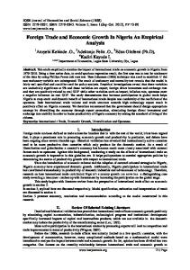
See Figure 1 for further details on the history of TAA certi…cations. Note, the certi…cation rate displayed in Figure 1 is below the …gures given above as the certi…cation rate reported by the DoL represents the percentage of petitions certi…ed over the number of petitions certi…ed or denied. In Figure 1, the denominator includes all petitions dispensed of in a given year (which includes those ‘terminated’and coded as ‘other’by the DoL). 9 Extended UI bene…ts provided under the TAA program are referred to as Trade Readjustment Allowances (TRA). 10 Of the 130 weeks of UI bene…ts under the 2002 Trade Act, 52 weeks (78 weeks of the 156 weeks under TGAAA) are available regardless of training participation. An additional 52 weeks and 26 weeks, respectively, are conditional on participation in occupational and remedial training. 11 Wage supplements/insurance is known as the Alternative Trade Adjustment Assistance (ATAA) program. To participate, workers must be over the age of 50, have been laid o¤ from a …rm having a signi…cant portion of workers at least 50 years old, lack easily transferable skills, and …nd a new job within 26 weeks of being laid o¤ that pays below $50,000 and below their prior wage. Workers meeting these criteria are then entitled to 50% of the shortfall between their new and prior salaries, up to a maximum of $10,000, for two years (US Government Accountability O¢ ce (2007)). However, participants must forego TAA-provided job training. These requirements and bene…ts were revised in 2009 under the TGAAA (US Government Accountability O¢ ce (2012a)).

5

tari¤ protection have a higher certi…cation rate. This does not seem consistent with the TAA program as a mechanism to redistribute the gains of trade liberalization from winners to losers. Thus, Magee concludes (p. 123) that “the evidence that TAA is being used to make trade liberalization Pareto-improving is inconclusive.” Our objective is to resolve this ambiguity by undertaking the …rst systematic investigation (to our knowledge) of whether TAA increases the politically viability of free trade via representative voting behavior. The second strand of related literature addresses the determinants of representative voting behavior on trade bills. Here, the role of trade-related redistribution has been ignored or overshadowed. For example, although not a main point of the paper, Conconi et al. (2012a) argue that factors a¤ecting the size of public transfers received by a CD (e.g., median family income) or levels of state-level redistribution (e.g., public spending on welfare, health, and education) have not driven US trade policy. In contrast, this literature has systematically investigated the role played by re-election considerations, local economic gains, and interest groups in determining Congressional voting behavior on trade policy. Conconi et al. (2014) investigate the role of re-election considerations. They …nd that the trade policy voting behavior of US Senators is more protectionist during the last 2-year cycle of their mandate, unless they face zero or very low re-election risk as a result of already announcing their retirement or being entrenched in a “safe seat”. Conconi et al. (2012b) and Conconi et al. (2012a) investigate the role of local economic gains. By examining votes since 1974 on fast track authority and all major trade-related bills, respectively, they …nd that voting behavior depends positively on a district’s potential gains from trade (proxied by, respectively, employment in export sectors divided by employment in import sectors within the district relative to the US as a whole or the share of residents with at least a Bachelor’s degree). In terms of the role played by interest groups, Baldwin and Magee (2000) …nd that political action committee (PAC) contributions by business and labor groups each have a statistically signi…cant e¤ect on voting behavior. Moreover, given the observed level of labor contributions, the analysis predicts that NAFTA would not have passed in the absence of the observed business contributions.12 Using …rm-level lobbying data, Ludema et al. (2011) analyze temporary tari¤ suspension bills brought before Congress from 19992006. The authors …nd that verbal opposition by groups whose opinion was sought by the US International Trade Commission outweighs the e¤ect of lobbying by proponents and opponents.13 12

Im and Sung (2011) follow the same empirical strategy for the seven US Congressional votes on FTAs between 2003 and 2006 and …nd similar results. 13 Although not a study of Congressional voting behavior, Bombardini and Trebbi (2009) also use …rm level lobbying data to explore the link between lobbying and trade policy. They focus on explaining inter-industry variation in protectionism by whether within-industry lobbying is primarily undertaken by individual …rms or collectively via trade associations.

6

3

Empirics

3.1

Theoretical Background

Our purpose in this section is to outline the political economy environment we envision that could produce a systematic relationship between expected trade-related redistribution and Congressional voting behavior. More generally, we sketch the motivations of Congressional representatives when voting on FTAs. Our starting point is a Congressional representative motivated by concerns for re-election (or election to higher o¢ ce). As such, the views of current constituents are an important determinant of representative voting behavior. To the extent that constituents’views are in‡uenced by the potential CD-level economic e¤ects of an FTA (both positive and negative) and expected redistribution from winners to losers under an FTA, these factors represent important determinants of representative voting behavior on FTAs. The CD-level economic e¤ects of an FTA, in turn, depend on the industrial composition of the CD and the structure of the local labor market. In terms of the structure of the local labor market, we assume a geographically immobile labor pool where unemployment is possible. In their online theory appendix, Autor et al. (2013) present a fullemployment model where labor is geographically immobile. This lack of geographical mobility has received signi…cant empirical support in Artuc et al. (2010), McLaren and Hakobyan (2012) and Autor et al. (2013). Further, Davidson and Matusz (2006) present a dynamic model featuring trade-induced unemployment. The authors model trade as displacing “low-tech” workers who then search for new employment in the “low-tech” sector or engage in training for “high-tech” jobs which allows them to search for new employment in the “high-tech” sector. This framework – combining geographical immobility and trade-induced unemployment – implies that workers at risk of trade-induced unemployment should take notice of FTA bills in Congress as well as TAA bene…ts that they may need.14 While Davidson and Matusz (2006) provide a useful framework to conceptualize our empirical analysis, the model does not outline the factors determining the magnitudes of trade-induced unemployment or employment. Upon FTA formation, we presume these magnitudes depend on six factors at the CDlevel: (i) the economic size of the FTA partner(s), (ii) the pre-FTA tari¤s imposed by the US on the FTA partner(s)15 , (iii) the pre-FTA tari¤s imposed by the FTA partner(s) on the US, (iv) the pattern of comparative advantage of the FTA partner(s) across sectors, (v) the pattern of US comparative advantage 14 Indeed, a 2010 Pew Research survey revealed 46% of respondents believed US FTAs had hurt the …nances of their own family (only 26% believed such agreements had helped) with these beliefs starker in older, less educated and lower income demographics. See http://www.people-press.org/2010/11/09/ public-support-for-increased-trade-except-with-south-korea-and-china/; accessed September 15 2014. Thus, it is very plausible that the median voter in many districts is one who believes they will be hurt by the FTAs entered into by the US. 15 Given various preferential tari¤ schemes such as the Generalized System of Preferences (GSP), the pre-FTA tari¤s imposed by the US may di¤er from the Most Favored Nation tari¤s of the US.

7

across sectors, and (vi) the industrial composition of the CD. All else equal, a CD with greater concentration of employment in US import-competing sectors is likely to experience a larger increase in unemployment when the pre-FTA tari¤s are higher and the FTA partner is more capable of taking advantage of the fall in tari¤s due its size and pattern of comparative advantage. Moreover, all else equal, a CD with greater concentration of employment in US export sectors is likely to experience a larger increase in employment when the pre-FTA tari¤s in the FTA partner(s) are higher and the US is more capable of taking advantage of the fall in tari¤s due its size and pattern of comparative advantage. Aside from these economic factors, we expect state-, CD-, and representative-level attributes to also in‡uence the voting behavior of representatives (see, e.g., Baldwin and Magee (2000)). At the representativelevel, political ideology, campaign contributions, and lobbying are likely to be salient. Campaign contributions and lobbying may a¤ect voting behavior on a quid-pro-quo basis (e.g. Grossman and Helpman (1994)) or because representatives use interest groups as a vehicle to extract relevant information (e.g. Austen-Smith (1995), Wright (1996)). At the state- and CD-level, demographic and economics attributes are likely to in‡uence political preferences and, hence, voting behavior.

3.2

Empirical Model

To assess the causal impact of expected trade-related redistribution on voting behavior, we formulate an empirical model that captures the relevant factors outlined in Section 3.1. Speci…cally, we estimate variants of the following speci…cation vidsbt = xit

1

+ xdt

2

+ xst

3

+ Rdt + e "idsbt ;

(1)

where vidsbt is the vote cast by representative i from CD d located in state s on FTA bill b in year t. This is a binary outcome, taking on the value of one (zero) if the representative votes in favor (against) the proposed FTA. The vectors xit , xdt , and xst denote vectors of representative-, CD-, and state-level covariates, respectively. Rdt is expected trade-related redistribution. Thus,

is the parameter of interest.

Finally, the composite error term, e "idsbt , includes both an idiosyncratic component, "idsbt , as well as various combinations of FEs. In our preferred speci…cation,

where

br

are FTA-by-region FEs and

e "idsbt = i

br

+

i

+ "idsbt ;

(2)

are representative FEs.16

Representative FEs are included in the model to control for time invariant unobserved heterogeneity that 16

We utilize eight regions based on the US Bureau of Economic Analysis (BEA) regional breakdown. See http://www.bea. gov/regional/docs/regions.cfm.

8

a¤ects voting behavior and may be correlated with the political or economic climate of a representative’s CD (Conconi et al. (2012a)). We use FTA FEs to help control for factors a¤ecting the economic impact of forming an FTA with a speci…c partner or partners (for example, the partner’s economic size). Further, allowing the FTA FEs to vary across regions helps control for additional geographical heterogeneity in the potential gains and losses from a particular FTA (due to, for example, distance to the country or countries in question). Since there are multiple FTA votes in some years, FTA FEs (as opposed to year FEs) are more comprehensive. The remaining covariates xit , xdt , xst and Rdt are discussed in the following section. We estimate (1) using a linear probability model (LPM) and cluster the standard errors at the representative level as in Ludema et al. (2011) and Conconi et al. (2012a). The LPM avoids the well-known incidental parameters problem that a¤ects some non-linear models, such as the probit model (Chamberlain (1984)). Some prior studies on voting behavior have utilized a FE logit model. However, the shortcoming with that model is that the average marginal e¤ects of the covariates cannot be computed because these depend on the FEs which are conditioned out of the likelihood function ((Wooldridge, 2010, p. 622-3)). We return to this later. Before turning to the next section, it is important to discuss potential threats to identi…cation. As discussed in Chappell (1982), Baldwin and Magee (2000), and Magee (2010), political money is not likely to be randomly assigned.17 For example, representatives that are visible proponents or opponents to trade liberalization may be more likely to receive funds from pro- or anti-trade groups, respectively. Such funds may be a mechanism to reinforce a representative’s existing views. Alternatively, representatives that are marginally inclined to vote one way may receive signi…cant funds from groups on the other side in an attempt to alter voting behavior. In this case, funds may be a mechanism to change a representative’s existing views. Moreover, political money is potentially measured with error as not all money given is necessarily trade-related and the data (discussed in the next section) do not allow us to perfectly …lter out funds associated with non-trade issues. While not the focus of this paper, if contributions, or measurement error in contributions, are correlated with expected redistribution (e.g., if pro-trade groups spend more when expected redistribution is low), then ignoring the endogeneity of political money will bias the estimate of . Although we do not think contributions are correlated with our measure of expected redistribution in practice, we revisit this issue below in Section 5.2. Expected redistribution may also be endogenous. Such concerns may arise for (at least) four reasons. First, consider the generosity of TAA bene…ts within a CD. One might worry that CDs may manipulate the level of bene…ts in order to in‡uence future trade votes. We do not believe this to be a source of bias. First, our measure of bene…ts is solely a function of a state’s UI system; there is no separate bene…t calculation for TAA recipients. Since TAA bene…ciaries represent a tiny fraction of the UI system, it is 17

See, however, Conconi et al. (2012a) for a recent paper treating political contributions as exogenous.

9

unlikely that states alter UI bene…ts in anticipation of future trade votes. For instance, state UI regular bene…t outlays were anticipated to be about $44 billion in 2013.18 There were 414,000 new UI claims in the week of December 14, 2013; nearly 2.9 million total claims.19 In contrast, only 81,000 workers were even eligible for TAA bene…ts in 2012 and the total cost of extended UI bene…ts received through the TAA program was less than $240 million. Second, even if states do adjust the level of UI generosity to sway upcoming votes, this does not lead to bias as

will re‡ect the causal impact of this variation in generosity

on voting behavior. Second, one might be concerned that expected redistribution is endogenous due to unobserved attributes correlated with both generosity and the propensity of representatives to vote in a particular direction on FTA bills (see, e.g., Magee (2001)). We also do not …nd this argument credible. First, our use of representative FEs and extensive controls for the political and local economic climate should adequately capture the underlying propensity of a representative to vote in favor of an FTA. Second, given TAA bene…ts are determined at the state level and given our host of FEs and control variables, temporal variation in generosity is unlikely to be correlated with unobserved temporal variation in the determinants of CD-level voting behavior. Third, one might be concerned that expected redistribution is endogenous due to spurious correlation between the likelihood of bene…t receipt and voting behavior. Speci…cally, there may be concern that the DoL is more lenient in its certi…cation decisions when new FTA bills are under consideration. That is, perhaps the DoL uses the certi…cation process to manipulate upcoming votes. Again, we do not believe this is an issue. First, we base our measure of the likelihood of future receipt on historical data (discussed in the next section). Second, our measure is based on the weighted average of the historical certi…cation rates across industries, where the weights represent the historical employment shares across industries within a CD. Consequently, our measure is not based on speci…c dealings with the TAA certi…cation process by individual representatives or their constituents. Third, as discussed above in relation to the possible manipulation of the UI system by states, we do not believe such manipulation by the DoL would introduce bias in our estimates. If the DoL is more likely to certify petitions made during periods leading up to a new FTA vote, our estimates of

will capture the causal e¤ect of this variation in certi…cation probability

on voting behavior. Nevertheless, again, we do not believe this is an issue. For example, Figure 1 shows that the years 2000-2006 represent seven of the eight years with the lowest certi…cation rate over the period 1992-2011, yet 2000-2006 was also a period where many FTAs were being negotiated and voted upon. Finally, our measure of expected redistribution may su¤er from measurement error. For example, representatives may form expectations concerning the expected take-up rate of TAA bene…ts by eligible 18 19

http://workforcesecurity.doleta.gov/unemploy/content/prez_budget.asp, accessed December 28, 2013. http://workforcesecurity.doleta.gov/unemploy/page8/2013/121413.html., accessed December 28, 2013.

10

constituents and incorporate such information into their perception of expected redistribution. Unfortunately, district-level data on historical take-up rates is not readily available. Ultimately, we do not believe expected redistribution is endogenous. However, as this is an empirical question, we test this in Section 5.2.

4

Data

Given the numerous data requirements needed to estimate (1), we pool together data from a large number of sources. Here, we provide cursory details of the data utilized. Table A1 in the appendix presents a more detailed description of the variables used and their sources. The appendix also contains a detailed description of the data construction process for select variables. The dependent variable – US Congressional voting behavior – is collected for all representative votes cast on each FTA bill brought before Congress between 1998 and 2013. We restrict the sample to the post-1998 period because lobbying data are unavailable prior to this. Table 1 lists the 11 FTA bills which form our sample, as well as the years and the breakdown of votes by party a¢ liation.20 Vote totals shown in Table 1 represent only those votes retained in our sample. There are a possible 435 votes in the House on each bill, for a total sample of 4785 votes. 16 votes are missing due to vacant seats at the time of the vote. 87 ‘non-votes’occurred despite the Congressional seat being occupied. 35 votes are omitted due to missing data on political money (see the appendix). Thus, our …nal sample includes 4647 votes.21 We de…ne expected trade-related redistribution as the product of two variables. The …rst measures the likelihood that a trade-displaced worker in a CD will gain TAA certi…cation. Since the usual predictor of future success is recent past experience, we compute a rolling, weighted average of past certi…cation rates across industries, where the weights re‡ect the employment shares in a given CD in 2000. Speci…cally, the expected probability of TAA certi…cation is de…ned as

Pdt =

X

! TjdRD

j2J T RD

"

tX 0 3

t=t0 1

njt Njt

#

(3)

where njt is the number of petitions from industry j that are certi…ed or partially certi…ed in year t and Njt is the total number of petitions from industry j that are ruled on (or withdrawn) in year t. Thus, the term in brackets represents the average certi…cation rate for a given industry over the three years preceding year t0 .22 J T RD represents the 441 4-digit SIC sectors engaged in trade (SIC codes 0111-3999). These 20 The US and Jordan entered into a FTA in 2001. However, only a voice vote was conducted; there is no record of the actual votes. Hence, the …rst FTA brought before Congress after 1998 that includes a vote record is the US-Chile FTA in 2003; so, our sample e¤ectively begins in 2003. 21 In Section 6 we further discuss the 87 non-votes. 22 We intentionally do not create a CD-level measure of past success based explicitly on TAA petitions involving …rms

11

SIC-speci…c certi…cation rates are then averaged using CD-speci…c weights, ! TjdRD . The weights are de…ned as Ejd;2000 j2J T RD Ejd;2000

! TjdRD = P

(4)

and represent the employment shares of each traded sector within a given CD in 2000. We utilize time invariant weights based on 2000 industrial composition since this pre-dates any of the FTA votes analyzed here and thus alleviates concerns that industrial composition may be a¤ected by passage of the FTAs being examined. The appendix provides more details on the data underlying (3) and (4). The second variable used to construct expected trade-related redistribution is the expected generosity of TAA bene…ts within a given CD. Since extended UI bene…ts are a major component of the TAA bene…ts, we borrow from the literature on UI bene…ts and utilize a standard measure of UI generosity: the replacement rate (see, e.g., Gruber (1997)). The replacement rate is de…ned as RRdt =

U Ist ; wst

(5)

where U Ist is the average weekly UI bene…t in state s during year t and wst is the average weekly wage. In the end, R in (1) is given by P

RR.

The remaining data corresponds to the representative, CD, and state covariates included in (1). Depending on the particular speci…cation, our representative covariates xit include party a¢ liation variables (not only party a¢ liation itself but also binary variables taking on the value of one if the representative is from the same political party as the president, the governor of one’s own state, and the majority party in the House of Representatives), gender, education level (less than a Bachelor’s degree, Bachelor’s degree, or advanced degree) and years since one …rst served as a member of the US House of Representatives.23 Our representative covariates also include controls for the in‡uence of interest groups. Speci…cally, we control for political money received by representative i which we de…ne as the sum of (i) trade-related contributions given to representative i and (ii) expenditures incurred by entities lobbying representative i on trade-related issues. Additionally we allow the e¤ect of political money to vary by party a¢ liation. While contributions data specify the recipient of an interest group’s contributions, it does not specify the interest group’s issue of concern. Conversely, while lobbying data specify the interest group’s issue of concern, it does not specify the representative targeted by lobbying expenditure. Thus, we take our measures from Lake (2015) who, essentially, (i) computes trade-related lobbying expenditures targeted at representative i by allocating an interest group’s trade-related lobbying expenditures across representatives in proportion to located within the CD. First, this would likely give rise to endogeneity concerns as discussed in Section 2. Second, there would be a signi…cant empty cell issue as many CDs have not had any workers covered by recent TAA certi…cations. 23 Note, party a¢ liation is time-varying due to the presence of some representatives who switch parties during the sample period.

12

the interest group’s allocation of PAC contributions across representatives, and (ii) computes trade-related contributions by allocating an interest group’s PAC contributions to a representative across issues (with trade being the issue we focus on) in proportion to the interest group’s allocation of lobbying expenditures across issues.24;25 Our CD-level covariates xdt largely consist of socioeconomic variables: population shares over the age of 25 by education (the percentage with less than a high school degree, high school degree, some college, and a Bachelor’s degree or higher), the unemployment rate of residents between 25 and 64 years of age for the same four education groups, and household median income. However, we also compute CD-level variables designed to capture the expected economic gains and losses from a particular FTA and allow the e¤ects of these variables to vary by party a¢ liation.26 We construct FTA-speci…c measures of what we refer to as local tari¤ vulnerability (LT V ) and local tari¤ gain (LT G). Local tari¤ vulnerability is a measure de…ned such that larger values denote CDs with higher employment shares in sectors with high pre-FTA tari¤s in which the proposed FTA partner(s) have a high revealed comparative advantage (RCA). Such CDs are considered most vulnerable to a particular FTA (McLaren and Hakobyan (2012) use a similar measure). Speci…cally, we begin with the pre-FTA tari¤ (at time t) imposed by the US on FTA partner b in sector j,

US b , jt

and weight this by the RCA of the

FTA partner in sector j, RCAbjt . We use the Proudman and Redding (2000) de…nition of RCAbjt which has a nice interpretation. RCAbjt exceeds one if and only if partner b’s share of world exports in sector j exceeds the partner’s average share of world exports across all sectors; thus, Proudman and Redding (2000) interpret RCAbjt > 1 as indicating that b specializes in sector j.27 Finally, we aggregate over all sectors using CD-industry employment shares to get our CD-level measure of local tari¤ vulnerability: LT Vdbt =

X

! jdt RCAbjt

US b : jt

(6)

j2J

where ! jdt is de…ned analogously to ! TjdtRD in (4) except that it is a weight over all 4-digit SIC sectors, J, and not only the traded sectors J T RD . Our measure of local tari¤ gain is de…ned analogously to (6): LT Gdbt =

X

S ! jdt RCAU jt

b US : jt

(7)

j2J

In words, CDs with high employment shares in sectors where the proposed FTA partner(s) have high pre-FTA tari¤s and the US has a high RCA are considered most likely to gain from a particular FTA. The 24

A category for “unallocated” contributions captures contributions made by groups that do not engage in lobbying. See the appendix for a more detailed explanation. 26 To be clear, we could actually use the notation xdbt rather than xdt because the local tari¤ vulnerability and local tari¤ gain measures are speci…c to the FTA partner(s) in bill b. 27 As described in the appendix, we exclude country b’s exports to the US when computing RCAbjt . 25

13

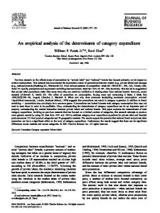
appendix contains more details about LT V and LT G including the data underlying these measures. Our state-level covariates xst include the political a¢ liation of the Governor, unemployment and employment rates, real per capita Gross State Product (GSP), the shares of agriculture and manufacturing in GSP, and union coverage within private manufacturing. Summary statistics are provided in Table 2. Table 3 displays a breakdown on the voting behavior of representatives in our sample across di¤erent FTAs. Since our preferred speci…cation incorporates representative FEs, as shown in (2), Table 3 highlights the within-representative variation in voting behavior used to identify the model. For example, of the 670 representatives appearing in our sample, 198 vote on all 11 FTAs we consider. One-third vote in favor of all 11; 15% vote against all 11. The remainder are fairly uniformly distributed between one and ten pro-FTA votes. Overall, 237 of the 670 representatives are observed casting both pro- and anti-FTA votes; 162 Democrats and 75 Republicans. Figure 2 depicts the spatial variation in voting behavior patterns across CDs.28

5

Results

5.1

Baseline Model

Select results from variants of the model in (1) are displayed in columns (1)-(3) of Table 4. Column (1) controls only for representative covariates (both time-varying and time invariant) as well as CD and FTA FEs. Column (2) replaces CD FEs with representative FEs. Finally, column (3) replaces FTA FEs with FTA-by-region FEs and adds CD and state covariates. Thus, column (3) is our preferred speci…cation of the baseline model. In each column, we present the coe¢ cient estimates for a subset of the covariates; the full set of results for the speci…cation in column (3) is provided in Table A2 of the appendix.29 The primary result from the speci…cations in columns (1)-(3) is that the coe¢ cient on expected redistribution is statistically signi…cant at least at the p < 0:10 con…dence level in all three speci…cations. Moreover, the point estimate is stable around 0.4. In terms of the magnitude of the e¤ect, in our preferred speci…cation (column (3)), we …nd that a ceteris paribus one SD increase in expected redistribution raises the probability of voting in favor of an FTA by roughly 1.8 percentage points on average. Thus, a one SD increase across all CDs raises the expected number of pro-FTA votes on a given bill by approximately eight. While statistically signi…cant, the magnitude of this average e¤ect indicates that modest variation in expected redistribution may not a¤ect the outcome of a given vote unless it is very close. The other coe¢ cients displayed in columns (1)-(3) in Table 4 are also interesting and informative. First, political a¢ liation is a strong predictor of voting behavior, as suggested in Tables 1 and 3. Speci…cally, 28 29

Representatives from Alaska and Hawaii voted against all FTAs on which they voted. The full set of results are available upon request.

14

all else held constant, Democrats are more than 50% less likely to vote in favor of an FTA.30 Second, while there does exist a weak positive statistical association between political money and pro-FTA votes for Republicans, the association is strongly positive (both statistically and economically) for Democrats.31 Third, local tari¤ vulnerabilities and potential local tari¤ gains matter, but in di¤erent ways for Republicans and Democrats. Republicans are responsive to local tari¤ vulnerability; greater vulnerability has a negative and statistically signi…cant e¤ect on the probability of voting in favor of an FTA for Republicans. The e¤ect is statistically insigni…cant for Democrats.32 Democrats, however, are responsive to local tari¤ gains; greater gains has a positive and statistically signi…cant e¤ect on the probability of voting in favor of an FTA for Democrats.33 The e¤ect is statistically insigni…cant for Republicans. While the coe¢ cient on local tari¤ gains for Democrats is smaller in absolute value than the coe¢ cient on local tari¤ vulnerability for Republicans, the scale of the local tari¤ gain variable is much larger. In actuality, the economic significance of each is not markedly di¤erent. Speci…cally, while a one SD decrease in local tari¤ vulnerability raises the likelihood of a Republican voting in favor of an FTA by 2.6 percentage points, a one SD increase in local tari¤ gains raises the likelihood of a Democrat voting in favor of an FTA by 3.2 percentage points. Before continuing to various extensions, we conduct two thought exercises to help quantify the economic signi…cance of expected trade-related redistribution. First, we compare the relative importance of local tari¤s and expected redistribution. For Republicans, we …nd that a 1.44 SD increase in expected redistribution is needed to o¤set a one SD increase in local tari¤ vulnerability in order to leave the probability of a pro-FTA vote unchanged (using the estimates in column (3)). For Democrats, we …nd that a 1.75 SD increase in expected redistribution is needed to o¤set a one SD decrease in local tari¤ gains in order to leave the probability of a pro-FTA vote unchanged (using the estimates in column (3)). Thus, the overall economic signi…cance of expected redistribution appears modest on average; it is less relevant than other economic considerations related to an FTA. For our second thought experiment, we estimate the ceteris paribus reduction in expected redistribution across all districts necessary to prevent the passage of each FTA. For US-CAFTA, which passed by a vote of 217-216, a 0.13 SD decline in expected redistribution across all CDs would have been su¢ cient to preclude passage (in expectation). For US-Oman, which passed by a vote of 218-212, a 0.79 SD decline would have been su¢ cient. However, for all other FTAs considered here, a ceteris paribus decline in expected redistribution to zero for all CDs still would not have altered the outcomes (in expectation) given the large 30

This result should be interpreted cautiously as the e¤ect of party a¢ liation is identi…ed in the models that include representative …xed e¤ects solely from two individuals who switch from Democrat to Republican during the sample period (Rodney Alexandar from Louisiana and Ralph Hall from Texas). Nonetheless, it is consistent with prior results in Blonigen and Figlio (1998), Baldwin and Magee (2000), Conconi et al. (2012b), and Conconi et al. (2012a). 31 Technically, the results for non-Democrats applies to Republicans and Independents. However, since Independents make up 0.2% of the sample, we simply refer to Republicans. 32 Note, the total e¤ect for a Democrat is 0:234 + 0:276 = 0:042 (p = 0:45) in column (3). 33 Note, the total e¤ect for a Democrat is 0:014 + 0:050 = 0:036 (p = 0:02) in column (3).

15

margins by which they passed. In sum, the results from our baseline model indicate that, in practice, the average e¤ect of expected redistribution is insu¢ cient to alter the political viability of free trade unless the vote is extremely close. In the following subsections, we assess the endogeneity of expected redistribution and political money, as well as examine potential sources of heterogeneity in the e¤ect of expected redistribution. Finally, in Section 6 we perform a variety of additional sensitivity analyses.

5.2

Endogeneity

We investigate two potential sources of endogeneity. First, as discussed above, political money may not be strictly exogenous. Funds may be used by an interest group to reinforce a representative’s already favorable stance towards the group’s policy preference. Alternatively, funds may be used in an e¤ort to sway a representative’s vote. Prior empirical evidence on the endogeneity of political money is mixed (e.g., Baldwin and Magee (2000)). To assess the sensitivity of our results concerning the impact of trade-related redistribution, we instrument for political money and political money interacted with Democrat using exclusion restrictions found in the existing literature. Following the spirit of Baldwin and Magee (2000) and Magee (2010), we utilize dummy variables indicating whether a representative is the chairperson of the Education and Workforce, Energy and Commerce, International Relations, or Ways and Means committee. We also create a dummy variable if the representative has been a member of the House for at least two years. These variables are designed to capture a representative’s legislative in‡uence. Finally, we follow the spirit of Ludema et al. (2011) and utilize contributions made to a representative related to issues other than trade. Intuitively, contributions made for non-trade reasons are indicative of a representative’s legislative power and fundraising ability. However, such contributions are unlikely to a¤ect voting on trade issues. Each instrument is also interacted with the dummy variable indicating if the representative is a Democrat. The results, based on a LPM, are presented in column (4) in Table 4.34 Before examining the coe¢ cient estimates, it is important to note that the instruments appear to do very well. The instruments are strongly related to the endogenous variables. We easily reject the null that the model is underidenti…ed at the p < 0:01 level according to the Kleibergen-Paap rk LM statistic. In addition, the Kleibergen-Paap rk Wald F -statistic exceeds 84. Finally, Hansen’s J test of overidenti…cation fails to reject the validity of the instruments (p > 0:82). Thus, the model appears to be well-speci…ed. In terms of the coe¢ cient estimates, two interesting …ndings emerge. First, the weak-instrument robust test of joint signi…cance of the endogenous regressors rejects the null that the coe¢ cients are jointly equal to zero at the p < 0:01 level. Thus, political money matters. However, examining the coe¢ cients indicates that political money matters only for Democrats; the combined coe¢ cient for Democrats is roughly 0.63 34

Estimation is performed via Generalized Method of Moments (GMM) using -xtivreg2- in Stata (Scha¤er (2010)).

16

and is statistically signi…cant at the p < 0:03 con…dence level. That said, the test of endogeneity, based on the di¤erence of two Sargan-Hansen statistics, fails to reject the null of exogeneity (p > 0:26). Second, as expected, the results pertaining to the e¤ect of expected redistribution are essentially unchanged. The same holds true for the other coe¢ cients reported (i.e., local tari¤ vulnerability and gains and party a¢ liation). The second potential source of endogeneity concerns the generosity of the UI system. As discussed previously, we do not believe unobserved attributes are correlated with both state UI bene…ts and representative preferences concerning FTA formation.35 Nonetheless, we instrument for expected redistribution using exclusion restrictions found in the labor literature. We utilize two instruments: the reserve ratio of the state UI system and the maximum weekly UI bene…t permitted in the state (each interacted with the prior TAA certi…cation rate). The UI reserve ratio is the year-end trust fund balance divided by total covered wages during the year. As discussed in Smith and Wenger (2013), the reserve ratio re‡ects the solvency of the state’s UI system and a¤ects the generosity of bene…ts. Conditional on our host of …xed e¤ects and control variables, we do not believe the solvency of the UI system is correlated with representative voting behavior on FTAs. In addition, following Krueger and Mueller (2010), we utilize the weekly maximum bene…t. The results are presented in column (5) in Table 4. Again, the instruments appear to perform well. We easily reject the null that the model is underidenti…ed at the p < 0:01 level according to the Kleibergen-Paap rk LM statistic. In addition, the Kleibergen-Paap rk Wald F -statistic exceeds 640. Finally, Hansen’s J test of overidenti…cation fails to reject the validity of the instruments (p > 0:19). In terms of the coe¢ cient estimates, very little changes. In fact, we again fail to reject the null of exogeneity (p > 0:52). That said, the coe¢ cient estimate on expected redistribution is no longer statistically signi…cant as it falls to closer to 0.3. Finally, in column (6) we instrument for political money and expected redistribution. Thus, we have three endogenous regressors. We utilize the combined set of instruments from the preceding speci…cations. Overall, the results do not di¤er much from those just described. The instruments continue to fare well according to the various speci…cation tests and, again, we fail to reject the null of exogeneity. In addition, the coe¢ cient estimates on political money are very similar to those in column (4), while the coe¢ cient estimate on trade-related redistribution variable is now closer to 0.4 and again statistically signi…cant at the p < 0:10 con…dence level. In sum, concerns related to the potential endogeneity of political money and expected redistribution do not have much empirical support. Our instrument sets perform very well in terms of their …rststage strength and excludability. However, the point estimates are relatively unchanged from the baseline 35

The best argument in favor of treating expected redistribution as endogenous is the presence of measurement error due to the fact that it may be an imperfect proxy for overall TAA generosity. We will return to this later.

17

speci…cations and we always fail to reject exogeneity. As such, the baseline speci…cations treating these variables as exogenous are preferred on e¢ ciency grounds.

5.3

Heterogeneous E¤ects of Redistribution

To this point, we have focused on the average e¤ect of expected redistribution on voting behavior. While we have documented a robust average e¤ect of expected redistribution on a representative’s likelihood to vote in favor of FTAs, the economic signi…cance is modest. However, the average e¤ect may disguise substantial heterogeneity across representatives in the e¤ect of expected redistribution on voting behavior. This is particularly true if the mechanism by which expected redistribution a¤ects voting behavior is through the compensation of potential losers from free trade. That is, one might expect redistribution to in‡uence a representative’s vote more when the FTA presents a greater economic risk for his or her constituents or when political conditions make a representative more sensitive to his or her constituents’concerns. We now explore possible sources of heterogeneity along these two dimensions. Formally, we now estimate models of the form vidsbt = xit

1

+ xdt

2

+ xst

3

+

where

idt

scalar,

1

5.3.1

Heterogeneity By Local Economic Conditions

0

idt Rdt

+e "idsbt ;

+ Zidt 1 , Zidt represents a vector of representative- and/or CD-level covariates,

(8) 0

is a

is a vector of scalars, and everything else is previously de…ned.

To begin, we treat Z as including measures of local economic conditions, the representative’s political party, and the interaction between the two. In terms of local economic conditions, we continue to use local tari¤ vulnerability and gains but also expand our analysis to include the CD unemployment rate and CD median household income. Since expected redistribution should a¤ect voting only in CDs which stand to lose from trade, or may be particularly worried about losing from trade, we expect the marginal e¤ect of expected redistribution to be large when local tari¤ vulnerability is high. To the extent that local economic concerns regarding FTAs are positively related to CD unemployment rates or negatively related to CD median household income, we again expect the marginal e¤ect of expected redistribution to be large in CDs with high unemployment rates or low median household income. Conversely, we expect the marginal e¤ect of expected redistribution to be independent of local tari¤ gains since, all else equal, expected redistribution is independent of whether a CD gains from an FTA via tari¤ reductions undertaken by the FTA partner(s). The results are presented in Table 5 and con…rm our expectations. Columns (1)-(3) of Table 5 view local economic conditions as the local tari¤ variables from our earlier analysis. Without allowing for heterogeneity by party a¢ liation, column (1) investigates how the e¤ect

18

of expected redistribution varies with local tari¤ vulnerability and local tari¤ gains. The coe¢ cient on expected redistribution,

0,

falls to 0.26 and is no longer statistically signi…cant. Thus, representatives

in districts una¤ected by an FTA (i.e., zero tari¤ vulnerability and tari¤ gains) are largely unmotivated by expected redistribution. Moreover, the interaction with local tari¤ gains is very close to zero and also statistically insigni…cant. As a result, the e¤ect of expected redistribution on voting behavior is independent of local tari¤ gains associated with the FTA. However, the e¤ect of expected redistribution on voting behavior depends strongly on the local tari¤ vulnerability faced by a representative’s constituents. Speci…cally, the interaction between expected redistribution and local tari¤ vulnerability is positive and statistically signi…cant. The estimates yield a marginal e¤ect for a representative from a CD with local tari¤ vulnerability at the 90th (10th ) percentile of 0.58 (0.26). The corresponding p-value at the 90th (10th ) percentile is 0.02 (0.27). Note, this more than twofold increase in the marginal e¤ect arises even though the di¤erence in local tari¤ vulnerability at the 90th and 10th percentiles is less than one SD.36 Stated di¤erently, the marginal e¤ect of a representative from a CD with local tari¤ vulnerability at the 90th percentile has a marginal e¤ect more than 48% greater than average marginal e¤ect reported in column (3) of Table 4. Further, the marginal e¤ect of expected redistribution evaluated at the mean value of local tari¤ vulnerability is approximately 0.38, very close to our baseline model result. These results suggest the positive e¤ect of expected redistribution that we consistently …nd in our baseline model estimating the average marginal e¤ect is, in fact, re‡ecting the underlying mechanism we believe to be operating. In columns (2) and (3) we investigate whether the heterogeneous marginal e¤ects just described also depend on party a¢ liation. The point estimates are consistent with Democrats being more sensitive to redistribution than Republicans when local tari¤ vulnerability is high.37 In addition, interactions with local tari¤ gains are very close to zero and not statistically signi…cant for either party. However, the imprecise estimates indicate that these results should be interpreted cautiously. Columns (4)-(7) now measure local economic conditions using either the CD unemployment rate (columns (4) and (5)) or CD median household income (columns (6) and (7)). These speci…cations are analogous to those in columns (1) and (3) where we viewed local economic conditions through the lens of local tari¤ vulnerabilities and gains. Ignoring any heterogeneity by party a¢ liation, the signs of the point estimates in columns (4) and (6) suggest larger marginal e¤ects of expected redistribution for representatives in CDs with higher unemployment rates and lower median household income. But, the economic signi…cance is weaker than in column (1). For a CD with an unemployment rate at the 90th percentile, the marginal is e¤ect is 0.43 (p = 0:26), roughly 9% higher than the baseline average e¤ect in Table 4. 36

Moreover, local tari¤ vulnerability at the 90th percentile is less than one SD above the mean. For example, the marginal e¤ect for a Democrat (Republican) from a CD with local tari¤ vulnerability at the 90th percentile is 0.63 (0.54). 37

19

For a CD with a median household income at the 10th percentile, the marginal is e¤ect is 0.52 (p = 0:07), roughly 32% higher than the baseline average e¤ect in Table 4. Given the imprecision, the results should be interpreted cautiously. In columns (5) and (7), we allow the heterogenous e¤ects of expected redistribution to depend on party a¢ liation. Again, although imprecise, the point estimates point to marginal e¤ects that are increasing (decreasing) in the local unemployment rate (median household income), particularly for Democrats. For a Democrat from a CD with an unemployment rate (median household income) at the 90th (10th ) percentile, the marginal e¤ect is 0.60 (0.62). Overall, the results in Table 5 provide strong evidence that there is signi…cant heterogeneity across representatives in the marginal e¤ect of expected redistribution on voting behavior. In particular, representatives from districts vulnerable to the FTA are most sensitive to expected redistribution. This is consistent with the underlying mechanism we believe to be operating: expected redistribution placates the constituents of representatives at-risk of su¤ering in the political arena from voting in favor of free trade. Moreover, the relatively more precise estimates obtained when measuring local economic conditions using local tari¤ vulnerability suggests that, as one may expect, this is a good proxy for local concerns over FTA formation. 5.3.2

Heterogeneity By Political Capital

The analysis in the preceding section shows that CDs vary in their vulnerability to FTAs and expected redistribution is more in‡uential in CDs that are more vulnerable to FTAs. This is intuitive to the extent that a representatives’ voting behavior depends on their constituent’s preferences. However, the extent that a representative internalizes his or her constituents’ preferences may depend on their re-election prospects. In particular, representatives who hold less “political capital” are presumably less able to withstand constituent unrest. In such cases, expected redistribution may be more in‡uential as it is necessary to squelch constituent unrest. Indeed, recent empirical evidence by Conconi et al. (2014) suggests a strong role for re-election motives in determining Congressional voting behavior on US trade policy. To this end, we now turn to speci…cations where Z includes various measures of a representative’s political capital, local economic conditions, and the interaction between the two. The measures of political capital we examine include a representative’s years of experience in the US House of Representatives, the representative’s margin of victory in the preceding general or special election, and the vote percentage received in the preceding general or special election.38 We anticipate that expected redistribution should have a larger in‡uence on the voting behavior of representatives with low political capital and this e¤ect 38 We examine the vote percentage in addition to the margin of victory since some elections contain more than two candidates. A special election refers to an election held during a Congressional cycle to replace a vacated seat.

20

should be magni…ed if local economic conditions are more dire. Table 6 presents the results and largely con…rms our expectations. To focus on heterogeneity by political capital, we initially abstract from any heterogeneity by local economic conditions. Columns (1), (5), and (9), allow the marginal e¤ect of expected redistribution to vary (non-linearly) with political capital. In each case, the impact of expected redistribution is highest for representatives with the least political capital. For example, in column (1), the marginal e¤ect exceeds unity for a representative with only one year of experience and declines monotonically until experience reaches roughly 50 years. In column (5), the marginal e¤ect is nearly unity for a representative who barely won the preceding election and declines monotonically to essentially zero for a representative who ran unopposed in the preceding election. In column (9), the marginal e¤ect is approximately unity for a representative who was elected with 45% of the vote in the prior election (again, a representative who barely won the prior election) and declines monotonically to essentially zero for a representative who ran unopposed in the preceding election. Note, a marginal e¤ect around one represents approximately a 150% increase over the baseline average marginal e¤ect in Table 4. Thus, we …nd strong evidence that the e¤ects of expected redistribution are strongest for representatives with the least political capital. This is consistent with the idea that these representatives are least able to withstand constituent unrest and, in turn, are most in‡uenced by the degree to which expected redistribution placates local concerns over FTA formation. The remaining speci…cations (columns (2)-(4), (6)-(8) and (10)-(12)) investigate whether the marginal e¤ect of expected redistribution varies simultaneously with political capital and local economic conditions. Before discussing these triple interactions, note that the point estimates (and statistical signi…cance) regarding the impact of political capital on the marginal e¤ect of expected redistribution are qualitatively similar to those reported in columns (1), (3) and (5). Speci…cally, the marginal e¤ect continues to decline with political capital. However, the coe¢ cients on the triple interactions (i.e., expected redistribution times political capital times local economic conditions) are imprecise and generally statistically insignificant. Nonetheless, the negative e¤ect of adverse local economic conditions continues to hold in most cases. To illustrate the results, Figure 3 plots the marginal e¤ect of expected redistribution as a function of the margin of prior electoral victory using the results in columns (6)-(8) for a CD with ‘good’and ‘bad’local economic conditions. Panel (a) con…rms our expectations. Greater local tari¤ vulnerability increases the marginal e¤ect of expected redistribution for any given level of political capital and also mutes the extent to which this marginal e¤ect declines with political capital. In Panel (b), we again see that worse local economic conditions, in the form of a higher unemployment rate, mutes the extent to which the marginal e¤ect of expected redistribution declines with political capital.39 In Panel (c), we see that the marginal 39

Note, the point estimate of the interaction between the unemployment rate and expected redistribution suggests this

21

e¤ect of expected redistribution is greater in districts with lower median household income conditional on any given level of political capital. However, unlike in Panels (a) and (b), adverse local economic conditions do not mitigate the extent to which this marginal e¤ect declines with political capital. In sum, the estimates in models with triple interactions involving political capital and local economic conditions tend to be imprecise. Thus, while the point estimates on interactions involving local economic conditions often con…rm our expectations, especially when viewing local economic conditions as local tari¤ vulnerability, these results should be treated cautiously. Nevertheless, the result that the marginal e¤ect of expected redistribution declines with political capital is quite robust, both economically and statistically. This is consistent with the underlying mechanism we believe to be operating: expected redistribution placates the constituents of representatives at-risk of su¤ering in the political arena from voting in favor of free trade.

6

Sensitivity Analyses

Before concluding, we conduct several additional analyses to explore the robustness of our results to various modeling choices. In the interest of brevity, we return to the baseline model where the focus is on the average marginal e¤ect of expected redistribution. This enables us to keep the number of speci…cations estimated within reason. Thus, our focus is on the speci…cation in column (3) in Table 4. Alternative Estimation Techniques As discussed above, we utilize LPMs to avoid the well-known incidental parameters problem (that plagues FE probit models) and enable estimation of average marginal e¤ects (which is not possible with FE logit models). As noted by Wooldridge (2010, p. 608), “[I]t is often useful to begin with a linear model with an additive, unobserved e¤ect.” As an alternative, we estimate a correlated random e¤ects (CRE) probit model. The bene…t of the CRE probit model is that it restricts the probability that v = 1 to the unit interval while allowing for correlation between the unobserved e¤ects and the covariates. In contrast to the LPM, the CRE probit model places some structure on the nature of this correlation. Formally, the ‘structural’model in the CRE probit model is given by Pr(vidsbt = 1 j Xidsbt ;

i)

= (Xidsbt +

br

+

i );

(9)

where Xidsbt includes the full set of covariates in (1), including our redistribution variables but omitting the intercept, and

is the standard normal cumulative density function. All other notation is de…ned

marginal e¤ect is greater in CDs with higher unemployment rates only if the representative has su¢ cient political capital. However, this point estimate is extremely imprecise.

22

previously. The Mundlak (1978) version of the CRE probit model further assumes

i

j Xidsbt

N(

0

+ X i 1;

2 a

where X i is the average of Xidsbt for each representative and i

=

0

+ Xi

1

2 a );

(10) is the variance of ai in the equation

+ ai .

Under (9) and (10), we obtain Pr (vidsbt = 1 j Xidsbt ) = =

h

(

0 + Xidsbt + a 0

a

+ Xidsbt

+

br + X i 1 ) a br

+ Xi

a 1

(1 +

2 1=2 a)

;

i

(11)

which is estimable using a population-averaged probit model (Wooldridge (2010)) where, for example, a 0

=

0

(1 +

2 ) 1=2 . a

E

Marginal e¤ects averaged over the distribution of a are then given by @ Pr(vidsbt = 1 j Xidsbt ) = @Xj

a j

(

a 0

+ Xidsbt

a

+

a br

+ X i a1 );

(12)

where E[ ] is the expectation operator taken over the distribution of the unobserved heterogeneity (a) and j indexes a continuous covariate included in X. The results are presented in column (1) in Table 7.40 The estimated e¤ects for local tari¤ vulnerability and gains, party a¢ liation, and expected redistribution are qualitatively similar to our prior results obtained using a LPM. Speci…cally, we …nd a negative e¤ect of local tari¤ vulnerability on the propensity of Republicans to vote in favor of an FTA, a positive e¤ect of local tari¤ gains on the propensity of Democrats to vote in favor of an FTA, as well as a negative direct association between being a Democrat and voting pro-trade. Furthermore, the e¤ect of redistribution is positive and the corresponding average marginal e¤ect is very close to the LPM estimate of 0.39. Although the estimate is imprecise, the result is consistent with a positive, but economically modest impact of expected redistribution on average. Our next alternative speci…cation alters the sample and estimation technique. Recall, 87 votes are missing despite the seat in Congress being …lled. To incorporate these ‘non-votes’, we de…ne the dependent variable, v, as zero for a vote against an FTA, one if the representative does not vote, and two for a vote in favor of an FTA. The choice of how to model v depends on whether one thinks of non-votes as a middle choice between yes and no (hence, v is an ordered outcome), or non-votes as simply an additional possible outcome (but v has no natural ordering). To decide, we …rst estimate a LPM using the same speci…cation as in column (3) in Table 4 except the outcome is one if the representative did not vote, zero otherwise. Of 40

The marginal e¤ect of expected redistribution is reported in the square brackets in Table 7.

23

the 107 parameters estimated, only two are statistically signi…cant at the p < 0:05 con…dence level.41 This is less than what one would expect by chance. Second, anecdotal evidence suggests that many instances of non-votes in our data appear driven by political formalities (e.g., the Speaker of the House does not typically vote if the vote is not expected to be close) or medical reasons (e.g., recovery from surgery or illness).42 Together, this suggests that non-votes are likely random and exogenous but, if modeled, should not be regarded as a deliberate behavioral choice; thus, we treat v as unordered. Estimating a CRE multinomial logit that treats di¤erent voting outcomes as unordered alternatives, we obtain average marginal e¤ects of expected redistribution on the probability of voting no (yes) of -0.27 (0.23) and on the probability of abstaining of 0.05.43 However, as with the CRE probit model, the estimates are imprecise. The standard error of each of the former is 0.28 and of the latter is 0.10. Alternative Measures of Expected Redistribution We now turn to investigations related to the measurement of expected redistribution. Given the preceding results concerning the use of the LPM and the endogeneity of key variables, we revert back to the original model in (1). However, now we alter our computation of a CD’s expected redistribution. To begin, we focus on the prior TAA certi…cation rate used in our measure. In our baseline model, the prior certi…cation rate is computed using a rolling window of the preceding three years, as shown in (3). Here, we experiment with di¤erent window widths. Column (2) in Table 7 utilize data from just the prior year (e.g., votes in 2003 depend on the certi…cation history from 2002). Column (3) utilizes a rolling window of the preceding …ve years. Column (4) utilizes a rolling window of the preceding ten years. Two primary results emerge. First, the coe¢ cients on the non-redistribution variables are essentially unchanged in all cases from the baseline speci…cations. Second, the impact of expected redistribution is nearly unchanged from our baseline model when we use the TAA certi…cation rate in just the prior year (column (2)). In fact, it is now statistically signi…cant at the p < 0:05 level. When we de…ne the prior TAA certi…cation over …ve or ten years, the coe¢ cients on expected redistribution are attenuated and no longer statistically signi…cant. This is consistent with the introduction of classical measurement error if we are mismeasuring expected redistribution by using a prior window that is wider than what guides expectations about certi…cation rates for voters and/or representatives. Next, we turn to the measure of TAA generosity used to create our measure of expected redistribution. 41 The two are the share of the population with some college and one FTA-by-region dummy. Results available upon request. 42 All 15 non-votes on the three FTA bills in 2011 fall into these two categories. 43 For comparison, we did estimate the model using a CRE ordered probit model, treating a non-vote as a middle choice. The results continue to be imprecise, but indicate a negative (positive) average marginal e¤ect of expected redistribution on the probability of voting against (for) an FTA (-0.13 and 0.14, respectively, with standard errors = 0.21). Unfortunately, there does not exist a test of whether the ordered probit model may be collapsed to a binary probit model (Franses and Cramer (2010)).

24

Speci…cally, the measure used in the baseline model accounts only for extended UI bene…ts. As noted earlier, job training, career services, relocation allowances, HCTC, and wage supplements represent a signi…cant portion of the bene…ts. Thus, our measure of TAA generosity is necessarily incomplete. However, the availability of these other bene…ts per recipient is unknown.44 That said, these bene…ts are paid for by federal transfers to the states using an allocation rule based on historical and anticipated usage but that is otherwise invariant across states.45 As a result, we assume that the expected value of these other bene…ts per eligible worker are constant across states and vary only by year. The expected level of TAA generosity is given by Bdt = RRdt + where

t

t;

(13)

is the (unobserved) expected level of expenditure per bene…ciary in year t on non-UI bene…ts

(normalized by the average wage so that RR and

are in comparable units).

Given this, the model we would like to estimate is vidsbt = xit where now R

where et

P

t.

1

+ xdt

2

+ xst

3

+ Rdt + e "idsbt ;

(14)

B. P is de…ned as before in (3). Substituting (13) into (14) yields vidsbt = xit

1

+ xdt

2

+ xst

3

= xit

1

+ xdt

2

+ xst

3

Given

t

+ [Pdt

(RRdt +

+ et Pdt + (Pdt

t )]

+e "idsbt

RRdt ) + e "idsbt ;

(15)

is unknown, estimating (15) entails interacting Pdt with a vector of year dummies

(since the coe¢ cient on Pdt now varies over time). Thus, despite

t

being unobserved, we can still recover

unbiased estimates of all parameters of the model. As such, for comparison to our baseline speci…cations, we can compute the marginal e¤ect, given by , of expected redistribution as determined by total bene…ts Bdt . The results are displayed in column (5) in Table 7. We obtain three key …ndings. First, the coe¢ cient 44

Individual-level data on the utilization of various bene…ts under the TAA are available through the Trade Act Participant Report (see, e.g., Park (2012)). However, even combining this with data on total federal funds allocated to each state, the data are not su¢ cient to derive a reasonable estimate of total state-level bene…ts per recipient – denoted by in (13) – that varies across states due to the fact that the funds allocated to each state are based on historical transfers and anticipated participation levels. Moreover, funds can be spent at any point over a three-year period (US Government Accountability O¢ ce (2007)). Thus, federal funds allocated to a state in a given year do not necessarily represent the level of funds spent on program participants. Roughly half of all states do place limits on the cost of training programs participants may attend. However, these are typically not binding (US Government Accountability O¢ ce (2007)). 45 The rough guidelines used to apportion funds for training to states are available at https://www.dol.gov/regulations/ taa-qa.htm. Funding rules used from 2004-2007 are described in US Government Accountability O¢ ce (2007). Prior to 2004, there were no codi…ed rules for allocating funds for training to states (US Government Accountability O¢ ce (2007, p. 65)). Currently, states are allocated funds at the start of the …scal year based on state-level trends in training participation over the previous four quarters for which data are available. Additional funds are allocated over the remainder of the year in response to unanticipated demand.

25

estimates are virtually unchanged. Second, we fail to reject the null that et is constant over time (p > 0:25).

This is consistent with the value of non-UI related TAA bene…ts being time invariant during the sample period. Third, while the e¤ect of expected redistribution is no longer statistically signi…cant, given the enormous increase in the standard errors, the point estimates are roughly 0.4 and thus unchanged from

our prior estimates. In sum, while it would be ideal to have location-speci…c data on the value of all TAA bene…ts, our focus on the generosity of extended UI bene…ts alone in the baseline speci…cations does not appear problematic. Finally, since our measure of expected redistribution combines both the extensive margin (i.e., the probability of bene…t receipt) and the intensive margin (i.e., bene…t generosity), it may be interesting to examine whether one margin matters more than the other. To that end, we estimate the following two speci…cations vidsbt = xit

1

+ xdt

2

+ xst

3

+

1 Pdt

+

2 RRdt

vidsbt = xit

1

+ xdt

2

+ xst

3

+

1 Pdt

+

2 RRdt

+e "idsbt +

3 Pdt

(16) RRdt + e "idsbt ;

(17)

where everything is previously de…ned. Note, whereas our baseline model given in (1) is nested in (17), the models in (1) and (16) are non-nested. The results, available upon request, do not allow us to draw any strong conclusions regarding the relative importance of the two margins. In both speci…cations, the coe¢ cients on the redistribution variables are individually and jointly statistically insigni…cant. However, in (17) we …nd that b1 and b2 are both negative, whereas b3 is large and positive. This suggests that both margins are important; only when both are strongly positive does expected redistribution have a positive impact on pro-FTA voting. Alternative Controls for Political Money Our …nal sensitivity analyses address the measurement of political money. In the baseline model, our political money variable comprised trade-related contributions and lobbying expenditures. Given the di¢ culty in parsing out trade-related and non-trade contributions and lobbying expenditures, we alternatively de…ne political money as the sum of all contributions and lobbying expenditures (i.e., trade plus non-trade plus unallocated) in column (6) in Table 7. The results are remarkably stable with the exception of coe¢ cients on political money. Now, the coe¢ cients on political money are extremely small although the pattern of relative magnitudes and statistical signi…cance remains the same as in the prior speci…cations. Moreover, since the SD of the new political money variable is roughly six times that of our trade-related political money variable, the marginal e¤ects of a one SD increase in political money is roughly identical to our baseline speci…cations. In column (7) in Table 7, we follow Baldwin and Magee (2000) and divide political contributions into

26

funds originating from business groups and funds originating from labor groups.46 Moreover, we follow Baldwin and Magee (2000) and now exclude lobbying expenditures. The results indicate a positive and statistically signi…cant e¤ect of business contributions received by Democrats. The remainder of the results are nearly identical to those in our baseline speci…cations.

7

Conclusion

There is a burgeoning literature in economics and political science on the determinants of voting behavior. Much of this literature focuses on the roles of political contributions and lobbying, information ‡ows to policymakers, and the welfare of constituents. In this study, we investigate a particular aspect of constituent welfare based on expected income transfers from winners to losers under policies with strong distributional implications. To our knowledge, the impact of such transfers on voting behavior has not been investigated empirically. However, this seems to be of …rst order importance as most policy reforms are not Pareto improving even if the net welfare gains are positive. Thus, while our analysis is in the context of trade policy, the implications are much broader. Our results indicate that redistribution under the auspices of the TAA program is, in fact, a statistically signi…cant determinant of the political viability of free trade. This e¤ect is remarkably stable across numerous sensitivity analyses. However, on average, the economic signi…cance of this e¤ect does not engender much belief that redistribution markedly a¤ects the political landscape. A one SD increase in expected trade-related redistribution raises the probability of voting in favor of an FTA by 1.8 percentage points. This is a much smaller impact than a one SD change in local tari¤ vulnerability or gains. Moreover, while a one SD reduction in expected redistribution across the entire US in 2005 and 2006 would have been su¢ cient to preclude the passage of CAFTA and the US-Oman FTA (in expectation), the complete elimination of the TAA would not have a¤ected the outcome of the other nine FTAs considered here. Thus, current levels of redistribution appear su¢ cient to break a deadlock, but otherwise have limited impact on voting behavior. That said, redistribution does matter in certain circumstances. In particular, it is has a large and statistically signi…cant e¤ect on the voting behavior of representatives from districts that are more vulnerable to tari¤ reductions under a particular FTA or have worse economic conditions. For example, a one SD increase in expected trade-related redistribution raises the probability of voting in favor of an FTA by 2.7 (1.2) percentage points for a representative from a district at the 90th (10th ) percentile in terms of local tari¤ vulnerability. In addition, representatives with little political capital are also more in‡uenced by redistribution. For instance, a one SD increase in expected trade-related redistribution raises the probability 46

The PAC contribution data obtained from the Center for Responsive Politics (see Appendix for more information) indicates the type of PAC. The possible types are business, labor, ideological, other, unknown or outside spending group.

27

of voting in favor of an FTA by 5.8 percentage points for a newly elected representative; it has no e¤ect on a representative who has served roughly 15 years. Finally, it should be noted that there is scope, if one wishes, to amend the TAA program in an e¤ort to ratchet up the e¤ect of redistribution on the political viability of free trade. Recent work assessing the e¤ectiveness of the TAA program using program data (Park (2012), Schochet et al. (2012)) suggests TAA could be more useful in terms of increasing political support for free trade. Moreover, as noted earlier, the take-up rate of bene…ts among eligible workers is less than 50%. On the other hand, it could be that extended UI bene…ts and job training may not be the optimal form of compensation for workers who su¤er due to trade. For example, Davidson and Matusz (2006) develop a model where trade adversely a¤ects not only workers who lose their jobs (and subsequently engage in costly search prior to re-employment), but also those in declining industries. The authors …nd that extended UI bene…ts and training is not the optimal compensation policy. Rather, wage subsidies for successful ‘switchers’and employment subsidies for ‘stayers’is optimal. Thus, future work should consider not only whether transfers improve the viability of policies which, even though not Pareto improving, yield net welfare gains but also the optimal form of such transfers (e.g. Brander and Spencer (1994), Kletzer (2004), Davidson and Matusz (2006)). Regardless, our results suggest that transfers from winners to losers are a modest component of the political economy story on average but a larger component for representatives whose constituents are particularly vulnerable to FTAs or representatives that face greater re-election risk.

References Aho, C. M., Bayard, T. O., 1984. Costs and bene…ts of trade adjustment assistance. In: The structure and evolution of recent US trade policy. University of Chicago Press, pp. 153–194. Ansolabehere, S., Snyder Jr, J. M., Tripathi, M., 2002. Are PAC contributions and lobbying linked? New evidence from the 1995 Lobby Disclosure Act. Business and Politics 4 (2), 131–155. Artuc, E., Chaudri, S., McLaren, J., 2010. Trade shocks and labor adjustment: A structural empirical approach. The American Economic Review 100 (3), 1008–1045. Austen-Smith, D., 1995. Campaign contributions and access. American Political Science Review 89 (03), 566–581. Autor, D. H., Dorn, D., Hanson, G. H., 2013. The China syndrome: Local labor market e¤ects of import competition in the United States. The American Economic Review 103 (6).

28

Baldwin, R. E., Magee, C. S., 2000. Is trade policy for sale? Congressional voting on recent trade bills. Public Choice 105 (1-2), 79–101. Bhagwati, J., 1989. Protectionism. The MIT Press. Blonigen, B., Figlio, D., 1998. Voting for protection: Does direct foreign investment in‡uence legislator behavior? The American Economic Review 88, 1002–1014. Bombardini, M., Trebbi, F., 2009. Competition and political organization: Together or alone in lobbying for trade policy? National Bureau of Economic Research Working Paper No. 14771. Bombardini, M., Trebbi, F., 2012. Competition and political organization: Together or alone in lobbying for trade policy? Journal of International Economics 87 (1), 18–26. Brander, J. A., Spencer, B. J., 1994. Trade adjustment assistance: Welfare and incentive e¤ects of payments to displaced workers. Journal of International Economics 36 (3), 239–261. Caliendo, L., Parro, F., 2015. Estimates of the trade and welfare e¤ects of NAFTA. The Review of Economic Studies 82 (1), 1–44. Chamberlain, G., 1984. Panel data. In: Z. Griliches, M. I. (Ed.), Handbook of Econometrics, Vol. 2. North-Holland, Amsterdam, pp. 1247–1318. Chappell, H., 1982. Campaign contributions and congressional voting: A simultaneous probit-tobit model. Review of Economics and Statistics 64, 77–83. Conconi, P., Facchini, G., Steinhardt, M. F., Zanardi, M., 2012a. The political economy of trade and migration: Evidence from the US Congress. HWWI Research Paper. Conconi, P., Facchini, G., Zanardi, M., 2012b. Fast-track authority and international trade negotiations. American Economic Journal: Economic Policy 4 (3), 146–189. Conconi, P., Facchini, G., Zanardi, M., 2014. Policymakers’horizon and trade reforms: The protectionist e¤ect of elections. Journal of International Economics 94, 102–118. Davidson, C., Matusz, S. J., 2005. Trade and turnover: theory and evidence. Review of International Economics 13 (5), 861–880. Davidson, C., Matusz, S. J., 2006. Trade liberalization and compensation. International Economic Review 47 (3), 723–747.

29

Davidson, C., Matusz, S. J., Nelson, D. R., 2007. Can compensation save free trade? Journal of International Economics 71 (1), 167–186. Dixit, A., Norman, V., 1986. Gains from trade without lump-sum compensation. Journal of International Economics 21 (1), 111–122. Dol…n, S., Berk, J., 2010. National evaluation of the Trade Adjustment Assistance program: Characteristics of workers eligible under the 2002 TAA program and their early program experiences. Mathematica Policy Research. Dol…n, S., Schochet, P., 2012. The bene…ts and costs of the Trade Adjustment Assistance (TAA) program under the 2002 amendments. Mathematica Policy Research. Feenstra, R. C., Lewis, T. R., 1994. Trade Adjustment Assistance and Pareto gains from trade. Journal of International Economics 36 (3), 201–222. Franses, P. H., Cramer, J. S., 2010. On the number of categories in an ordered regression model. Statistica Neerlandica 64 (1), 125–128. Furusawa, T., Lai, E. L.-C., 1999. Adjustment costs and gradual trade liberalization. Journal of International Economics 49 (2), 333–361. Grossman, G., Helpman, E., 1994. Protection for sale. American Economic Review 84 (4), 833–850. Gruber, J., 1997. The consumption smoothing bene…ts of unemployment insurance. The American Economic Review 87 (1), 192–205. Hummels, D., Ishii, J., Yi, K.-M., 2001. The nature and growth of vertical specialization in world trade. Journal of international Economics 54 (1), 75–96. Im, H., Sung, H., 2011. Empirical analyses of US Congressional voting on recent FTA. The BE Journal of Economic Analysis & Policy 11 (1). Kletzer, L., 1998. Job displacement. The Journal of Economic Perspectives 12 (1), 115–136. Kletzer, L., Rosen, H., 2005. Easing the adjustment burden on us workers. In: Bergsten, C. (Ed.), The United States and the World Economy: Foreign Economic Policy for the Next Decade. Institute for International Economics, pp. 313–342. Kletzer, L. G., 2004. Trade-related job loss and wage insurance: A synthetic review. Review of International Economics 12 (5), 724–748.

30

Krueger, A., Mueller, A., 2010. Job search and unemployment insurance: New evidence from time use data. Journal of Public Economics 94, 298–307. Lake, J., 2015. Revisiting the link between PAC contributions and lobbying expenditures. European Journal of Political Economy 37, 86–101. Lawrence, R. Z., Litan, R. E., 1986. Saving free trade: A pragmatic approach. Brookings Institution Washington, DC. Ludema, R., Mayda, A. M., Mishra, P., 2011. Protection for free: The political economy of US tari¤ suspensions. Mimeo. Magee, C., 2001. Administered protection for workers: an analysis of the Trade Adjustment Assistance program. Journal of International Economics 53 (1), 105–125. Magee, C., 2010. Would NAFTA have been approved by the House of Representatives under President Bush? Presidents, parties, and trade policy. Review of International Economics 18 (2), 382–395. McLaren, J., Hakobyan, S., 2012. Looking for local labor market e¤ects of NAFTA. National Bureau of Economic Research Working Paper No. 16535. Mundlak, Y., 1978. On the pooling of time series and cross section data. Econometrica 46 (1), 69–85. Park, J., 2012. Does occupational training by the Trade Adjustment Assistance program really help reemployment? Success measured as occupation matching. Review of International Economics 20 (5), 999– 1016. Proudman, J., Redding, S., 2000. Evolving patterns of international trade. Review of International Economics 8 (3), 373–396. Rodrik, D., 1998. Why do more open economies have bigger governments? Journal of Political Economy 106 (5), 997–1032. Romalis, J., 2007. NAFTA’s and CUSFTA’s impact on international trade. The Review of Economics and Statistics 89 (3), 416–435. Scha¤er, M., 2010. xtivreg2: Stata module to perform extended iv/2sls, gmm and ac/hac, liml and k-class regression for panel data models. http://ideas.repec.org/c/boc/bocode/s456501.html. Scheve, K. F., Slaughter, M. J., 2001. Globalization and the perceptions of American workers. Peterson Institute.

31

Schochet, P., D’Amico, R., Berk, J., Dol…n, S., Wozny, N., 2012. Estimated impacts for participants in the Trade Adjustment Assistance (TAA) program under the 2002 amendments. Mathematica Policy Research. Smith, D., Wenger, J., 2013. State unemployment insurance trust solvency and bene…t generosity. Journal of Policy Analysis and Management 32 (3), 536–553. Stein, L., 1982. Trade Adjustment Assistance as a means of achieving improved resource allocation through freer trade: An analysis of policies for aiding the import-injured in the US, Canada and Australia. American Journal of Economics and Sociology 41 (3), 243–255. US Department of Labor, 2012. Fiscal year 2012 report to the Committee on Finance of the Senate and Committee on Ways and Means of the House of Representatives. US Government Accountability O¢ ce, 2007. Trade Adjustment Assistance: Changes to funding allocation and eligibility requirements could enhance states’ability to provide bene…ts and services. US Government Accountability O¢ ce, 2012a. Trade Adjustment Assistance: Changes to the workers program bene…ted participants, but little is known about outcomes. US Government Accountability O¢ ce, 2012b. Trade Adjustment Assistance: Commerce program has helped manufacturing and services …rms, but measures, data, and funding formula could improve. Viner, J., 1950. The Customs Union issue. Carnegie Endowment for International Peace, New York. Wooldridge, J. M., 2010. Econometric analysis of cross section and panel data, 2nd Edition. The MIT press. Wright, J. R., 1996. Interest groups and Congress: Lobbying, contributions, and in‡uence. Allyn and Bacon Boston.

Appendix Table A1 in this appendix de…nes the variables used and provides their sources. Here, we provide a more detailed description of data construction process for select variables. Expected trade-related redistribution Expected trade-related redistribution is the product of two variables: CD-level prior TAA certi…cation rate and the UI replacement rate. The replacement rate is straightforward; however, the CD-level prior TAA certi…cation requires further explanation. This variable 32

is a rolling, weighted average of past certi…cation rates across industries, where the weights re‡ect the employment shares in a given CD in 2000. As noted in the text, this variable is de…ned as

Pdt =

X

! TjdRD

j2J T RD

"

tX 0 3

t=t0 1

njt Njt

#

where nj is the number of petitions from industry j that are certi…ed or partially certi…ed in year t and Njt is the total number of petitions from industry j that are ruled on (or withdrawn) in year t. J T RD represents the 441 4-digit SIC sectors engaged in trade (SIC codes 0111-3999). These SIC-speci…c certi…cation rates are then averaged using CD-speci…c weights, ! TjdRD . The weights are de…ned as Ejd;2000 j2J T RD Ejd;2000

! TjdRD = P

and represent the employment shares of each traded sector within a given CD in 2000. The data on the disposition of TAA petitions is from the DoL. Each petition is assigned a unique identi…cation number, and the data include the decision date, DoL decision, and the 4-digit SIC of the …rm covered by the petition. The data on CD-level employment shares in 2000 are derived from the Quarterly Census of Employment and Wages (QCEW). To align with the TAA petition data at the 4-digit SIC level, we convert the QCEW data to 4-digit SIC industries using concordances from the US Census Bureau.47 We then use concordances from the Missouri Census Data Center for the 108th and 109th Congresses and from the US Census Bureau for the 110th Congress to convert the data from the county-level to the CD-level.48 Local tari¤ vulnerability and local tari¤ gain In terms of the CD-level covariates, the local tari¤ vulnerability and gain variables merit further explanation. As noted in the text, local tari¤ vulnerability captures the expected average tari¤ decline in a given CD adjusted to account for the industrial composition of CDs, sector-speci…c pre-FTA tari¤s imposed on the proposed FTA partner(s), and the sector-speci…c revealed comparative advantage (RCA) of the proposed FTA partner(s) (see, e.g., McLaren and Hakobyan (2012)). Formally, de…ne the employment share of sector j in district d in 2000 as Ejd;2000 j2J Ejd;2000

47

! jd = P

http://www.census.gov/eos/www/naics/concordances/concordances.html Missouri Census Data Center concordances can be found at http://mcdc.missouri.edu/websas/geocorr2k.html. Census concordances can be found at http://www.census.gov/geo/maps-data/data/cd_state.html. Unlike the Census, the Missouri Census Data Center allows users to download concordances for all states at once. However, the Missouri Census Data Center does not provide concordances for the 110th Congress when only Texas and Georgia engaged in redistricting. There was no redistricting for the 111th Congress which is the last Congress in our sample. The concordances give population allocation shares for counties which lie in multiple districts. We use these as weights when allocating a county’s employment level in a given sector across across districts (see, e.g., Conconi et al. (2012b)). 48

33

where J represents all 4-digit SIC sectors. Then, local tari¤ vulnerability, LT V , is de…ned as LT Vdbt =

X

! jd RCAbjt

US b jt

j2J

where RCAbjt is the RCA of the proposed partner(s) in FTA bill b in sector j in year t and

US b jt

is the

pre-FTA tari¤ imposed by the US on imports from the proposed partner(s) in FTA bill b in sector j in year t.49,50 With one minor di¤erence, we use the Proudman and Redding (2000) de…nition of RCAbjt . The Proudman and Redding (2000) measure is:

RCAbjt =

xjb PJ

1 J

j=1 xjb

where Xjb denotes country b’s exports of sector j to the world and xjb = Xjb =

PJ

j=1 Xjb

denotes sector j’s

share of country b’s exports to the world. Our measure of RCAbjt di¤ers from this only because we de…ne Xjb as country b’s exports of sector j to the world excluding the US as an export destination. In either P case, it is simple to verify that J1 Jj=1 RCAbjt = 1. Our local tari¤ gain measure is analogous, but re‡ects the expected average tari¤ decline in the proposed

FTA partner(s) adjusted to account for the industrial composition of CDs, sector-speci…c pre-FTA tari¤s faced by the US in the proposed FTA partner, and the sector-speci…c revealed comparative advantage (RCA) of the US. Formally, local tari¤ gain, LT G, is de…ned as X

S ! jd RCAU jt

b US jt

S where RCAU jt is the RCA of the US in sector j in year t and

b US jt

LT Gdbt =

j

is the pre-FTA tari¤ on US exports

S in the proposed partner(s) in FTA bill b in sector j in year t. Analogous to RCAbjt , RCAU jt is given by

S RCAU jt =

1 J

xjU S PJ j=1 xjU S

where XjU S denotes US exports of sector j to the world excluding FTA partner(s) b as export destinations P and xjU S = XjU S = Jj=1 XjU S denotes sector j’s share of US exports to the world (again, excluding FTA partner(s) b as export destinations).

Computation of LT V and LT G requires data on pre-FTA tari¤s imposed by the US on the FTA 49

We treat the RCA of non-traded sectors as zero. We treat the industry j pre-FTA tari¤ imposed by the US on CAFTA-DR as a trade weighted average across the CAFTADR countries where a country’s weight is that country’s share of total industry j exports from CAFTA-DR to the US. Similarly, we use US export shares to construct the industry level pre-FTA tari¤s imposed by CAFTA-DR on the US. 50

34

partner(s) and vice versa, export data, and CD-level employment shares in 2000 (described above). All data are available at the 4-digit SIC level. Export data are obtained from the COMTRADE database within the World Bank’s Integrated Trade Solution (WITS) database. The 4-digit SIC tari¤ data are also from the WITS database. Where possible, we use the TRAINS data set within WITS for tari¤s since it provides ad valorem equivalent tari¤s (which convert non ad valorem tari¤s into an ad valorem rate).51 Often, the pre-FTA tari¤s imposed by the US on FTA partners are below the Most Favored Nation (MFN) level due to non-reciprocal preferential schemes such as the Generalized System of Preferences. Political money

In terms of the representative-level covariates, political money is the most complex.

We take our measures from Lake (2015), but we present a self-contained description here. Data on a representative’s political money comes from the Center for Responsive Politics (CRP). The objective is to construct a measure of (i) trade-related contributions given to each representative and (ii) expenditures incurred by entities lobbying each representative on trade-related issues. For each two-year Congressional election cycle, data are available on the PAC contributions received by a representative. In addition, the lobbying expenditures incurred by any interest group mandated to …le Federal lobbying expenditure reports under the 1995 Lobbying Disclosure Act (either because it hired a …rm to lobby on its behalf or because it employed in-house lobbyists) are available. As discussed by Bombardini and Trebbi (2012), the shortcoming with the contributions data is that a given PAC may be concerned with multiple issues and thus not all of the contribution represents a ‘trade-related’gift.52 The quarterly …led lobbying expenditure reports, on the other hand, must include the issues lobbied on from a pre-de…ned list of issues; trade is one issue. Nevertheless, the lobbying data has its own shortcoming: the politicians being lobbied are not included. Thus, the contributions data contains the representatives being targeted, but not the issue of concern, whereas the lobbying data contains the issue of concern, but not the representatives being targeted. These shortcomings can be dealt with by utilizing the fact that the majority of PAC contributions come from interest groups who also lobby and the majority of lobbying expenditures accrue from interest groups who also give PAC contributions (Ansolabehere et al. (2002), Lake (2015)). As such, most political money comes from ‘groups’for which the data contains (i) their contributions given to individual representatives and (ii) their total trade-related lobbying expenditures. This information can be used to compute separate values for the amount of trade-related contributions and trade-related lobbying received by each 51

For Morocco’s tari¤s in 2004, there is no data in the WITS database (either TRAINS or WTO) so we use the TRAINS tari¤s from 2003. For Panama and Korea, the last pre-FTA tari¤s in TRAINS are in 2007 even though there are 2011 WTO tari¤s. However, the WTO tari¤s are not advalorem equivalent. So for each sector j we compute the ratio of the ad valorem equivalent tari¤ to the ad valorem tari¤ in 2007 using the TRAINS dataset, say j , and then multiply the WTO 2011 tari¤ in sector j by j to get an imputed ad valorem equivalent tari¤. 52 Because of this, Ludema et al. (2011) omit contributions from their analysis and focus solely on lobbying expenditures.

35

representative.53 Speci…cally, start with the contributions given to House representative i by group g in period t, denoted Cigt , and the lobbying expenditures on issue k by group g in period t, denoted Lkgt .54,55 Note that even though the lobbying data does not detail the representatives targeted, it does detail the government agencies lobbied (e.g. House, Senate, O¢ ce of US Trade Representative). Additionally, any lobbying report …led only details the total lobbying expenditure for the …ling period (quarterly or semi-annually) and the list of issues lobbied. Thus, divide the lobbying expenditure on a report equally between all issues and agencies lobbied and, abusing notation, rede…ne Lkgt as relating to expenditures targeted at House representatives. Then, compute the share of group g’s contributions (to House representatives) going to representative i in period t, denoted cigt = period t devoted to trade, denoted lk

gt

PCigt , i Cigt Lk gt

= X

k

and the share of group g’s lobbying expenditures in where k

trade. Next, compute the trade-related

Lkgt

contributions received by representative i in period t as Cittrade =

X

lobbying expenditure spent on representative i in period t as Ltrade = it

lk g X g

gt Cigt

cigt Lk

and the trade-related gt .

Finally, sum Cittrade

and Ltrade to form a representative’s total trade related political money; we refer to this variable in the it tables as “Political Money”.

53

Our approach of tying trade-speci…c lobbying expenditures to representative recipients distinguishes our use of lobbying expenditures from others, such as Bombardini and Trebbi (2012), who analyze lobbying from the perspective of the lobbying …rm. Our trade-related contribution and trade-related lobbying expenditure measures are publicly available on the website of the corresponding author (analogous variables are available there for each of the 79 possible lobbying issues). 54 Like Baldwin and Magee (2000), political money associated with a representative’s vote in a given year is that expended in the election cycle leading upto the current Congress. In other words, voting behavior in, say, 2003 and 2004 is assumed to depend on lobbying and contributions made leading up to one’s election in Fall 2002. This timing issue explains why we have missing data on political money for 35 votes in our sample. These 35 votes are cast by representatives who were not elected, but rather appointed mid-term to …ll a vacant seat. As a result, there is no data on the political money raised by these individuals during the preceding election cycle. 55 In the CRP dataset, contributions given to the representative are “direct contributions”. This contrasts with “indirect contributions” which are spent on behalf of the representative.

36

4000 1000 2000 3000 Number of Petitions

.8 Petition Certification Rate .2 .4 .6

0

0

1975

1980

1985

1990

Certification Rate

1995 Year

2000

2005

2010

2015

Number of Petitions

Figure 1. TAA Certification History. Note: Certification rate is based on the number of petitions either certified or partially certified out of all petitions dispensed of during a given year. The total number of petitions includes all petitions dispensed of in a given year, including those coded as ‘terminated’ or ‘other’ by the US Department of Labor.

Figure 2. Congressional District Voting Behavior. Note: The figure depicts the proportion of FTA votes in our sample that a Congressional districts’ representative(s) cast in favor of proposed FTAs.

2 Marginal Effect of Expected Redistribution .5 1 1.5 0 0

.1

.2

.3

.4 .5 .6 .7 Previous Margin of Victory

.8

.9

1

.8

.9

1

.8

.9

1

Local Tariff Vulnerability = 0 Local Tariff Vulnerability = 0.5

-.5

Marginal Effect of Expected Redistribution 0 .5 1

1.5

(a)

0

.1

.2

.3

.5 .6 .7 .4 Previous Margin of Victory Unemployment Rate = 0 Unemployment Rate = 10%

-.5

Marginal Effect of Expected Redistribution 0 .5

1

(b)

0

.1

.2

.3

.7 .4 .5 .6 Previous Margin of Victory Median HH Income = $50k Median HH Income = $100k

(c) Figure 3. Heterogeneous Effects of Expected Redistribution. Note: Figures based on columns (6)-(8) in Table 7.

Table 1. Breakdown of Votes by FTA Vote

Independent

Political Party Democrat

Republican

Total

US-Chile (2003)

N Y

1 0

128 74

27 194

156 268 424

US-Singapore (2003)

N Y

1 0

127 74

27 196

155 270 425

US-Australia (2004)

N Y

1 0

82 116

24 196

107 312 419

US-Morocco (2004)

N Y

1 0

79 118

18 201

98 319 417

US-Bahrain (2005)

N Y

1 0

81 114

13 211

95 325 420

US-CAFTA (2005)

N Y

1 0

186 15

27 202

214 217 431

US-Oman (2006)

N Y

1 0

175 22

28 196

204 218 422

US-Peru (2007)

N Y

0 0

114 109

16 175

130 284 414

US-Colombia (2011)

N Y

0 0

156 31

9 229

165 260 425

US-Panama (2011)

N Y

0 0

121 66

6 232

127 298 425

US-South Korea (2011)

N Y

0 0

128 59

21 216

149 276 425

Notes: Vote totals differ across FTAs due to non-votes and vacant seats. Votes represent those included in our sample. Some votes are excluded due to missing covariates used in the analysis.

Table 2. Summary Statistics. Variable

Mean

SD

Min

Max

FTA Vote (1 = Yes, 0 = No) Expected Redistribution

0.656 0.189

0.475 0.046

0 0.025

1 0.361

10.127 0.382 0.681 0.002 0.468 0.530 0.852 0.072 0.288 0.640 0.002 0.002 0.002 0.002 67130.7 90938.5 365955.9 399177.9 0.498 0.537 0.530

8.420 0.253 0.129 0.039 0.499 0.499 0.355 0.259 0.453 0.480 0.049 0.049 0.049 0.049 65629.8 96268.0 287457.8 255594.3 0.500 0.499 0.500

0 0.0003 0.450 0 0 0 0 0 0 0 0 0 0 0 -1007.3 -5949.8 -2974.9 -5860.7 0 0 0

46 1 1 1 1 1 1 1 1 1 1 1 1 1 650899.8 507753.5 2408148.0 2462440.0 1 1 1

District Covariates Local Tariff Vulnerability Local Tariff Gain Education, % HS Graduate (Aged 25+) Education, % Some College (Aged 25+) Education, % BA (Aged 25+) Education, % Advanced Degree (Aged 25+) UR (Aged 25-64) UR, Less than HS (Aged 25-64) UR, HS (Aged 25-64) UR, Some College (Aged 25-64) UR, BA or Higher (Aged 25-64) Median Household Income ($/100,000)

0.038 0.534 0.295 0.075 0.172 0.100 6.309 12.145 7.792 6.148 3.331 0.507

0.111 0.876 0.065 0.016 0.056 0.046 2.479 5.047 3.288 2.602 1.416 0.175

0 0 0.119 0.031 0.044 0.016 2.1 2.0 1.5 1.7 0.5 0

3.582 15.371 0.494 0.131 0.370 0.312 21.7 38.8 28.2 21.0 11.3 1.173

State Covariates Governor (1 = Independent) Governor (1 = Democrat) Governor (1 = Republican) Real GSP (Per Capita, 2005$) Agriculture (% of GSP) Manufacturing (% of GSP) Unemployment Rate Employment Rate Union Coverage (%, Private Manufacturing) UI Reserve Ratio UI Weekly Maximum Benefit

0.005 0.449 0.546 0.042 0.010 0.127 6.320 0.576 12.058 0.005 397.659

0.072 0.497 0.498 0.006 0.009 0.052 2.021 0.036 6.384 0.008 110.677

0 0 0 0.028 0.001 0.015 2.500 0.480 1.200 -0.008 200

1 1 1 0.065 0.098 0.366 13.200 0.766 31.300 0.037 937

Member Covariates Experience Margin of Victory Vote Percentage Independent (1 = Yes) Democrat (1 = Yes) Republican (1 = Yes) Gender (1 = Male) Education (1 = Less than BA Degree) Education (1 = BA Degree) Education (1 = Advanced Degree) Committee Chair (1 = Education & Workforce Committee Chair (1 = Energy & Commerce) Committee Chair (1 = Int'l Relations) Committee Chair (1 = Ways & Means) Political Money (2010 US$) Labor Contributions (2010 US$) Business Contributions (2010 US$) Non-Trade Political Contributions (2010 US$) Same Party as President (1 = Yes) Same Party as House Majorty (1 = Yes) Same Party as Governor (1 = Yes)

Notes: N = 4647. Data cover votes on 11 Free Trade Agreements (FTAs) over the period 2003-2011 in the House of Representatives. UI = Unemployment Insurance. TAA = Trade Adjustment Assistance. BA = Bachelor's. HS = High School. UR = Unemployment Rate. GSP = Gross State Product. See text for sources and other details.

Table 3. Distribution of Votes Across Representatives Number of Votes Cast by a Representative I. Full Sample 1 2 3 4 5 6 7 8 9 10 11

0

1

0.52 0.20 0.15 0.21 0.13 0.13 0.16 0.08 0.33 0.16 0.15

0.48 0.00 0.03 0.07 0.00 0.07 0.01 0.08 0.00 0.05 0.08

II. Democrats 1 2 3 4 5 6 7 8 9 10 11

0.65 0.50 0.58 0.39 0.20 0.20 0.45 0.16 0.50 0.30 0.26

0.35 0.00 0.11 0.13 0.00 0.20 0.05 0.16 0.00 0.10 0.14

III. Non-Democrats 1 0.00 2 0.00 3 0.02 4 0.00 5 0.00 6 0.10 7 0.05 8 0.02 9 0.00 10 0.00 11 0.01

1.00 0.00 0.00 0.00 0.00 0.00 0.00 0.02 0.00 0.00 0.00

2

0.80 0.11 0.09 0.25 0.00 0.06 0.04 0.00 0.00 0.04

0.50 0.19 0.16 0.20 0.00 0.23 0.07 0.00 0.00 0.06

1.00 0.08 0.00 0.33 0.00 0.00 0.02 0.00 0.00 0.00

3

0.72 0.10 0.13 0.07 0.02 0.05 0.33 0.11 0.04

0.11 0.08 0.20 0.20 0.00 0.09 0.50 0.20 0.05

0.90 0.13 0.00 0.00 0.03 0.02 0.00 0.00 0.01

Number of Pro-FTA Votes 4 5 6 7

0.53 0.13 0.13 0.04 0.05 0.00 0.00 0.06

0.24 0.20 0.20 0.05 0.04 0.00 0.00 0.10

0.88 0.00 0.10 0.03 0.06 0.00 0.00 0.01

0.38 0.13 0.13 0.06 0.00 0.00 0.05

0.20 0.20 0.18 0.09 0.00 0.00 0.06

0.67 0.10 0.12 0.04 0.00 0.00 0.03

0.47 0.09 0.08 0.00 0.00 0.04

0.20 0.00 0.18 0.00 0.00 0.06

0.70 0.12 0.00 0.00 0.00 0.01

0.49 0.09 0.00 0.16 0.02

0.05 0.13 0.00 0.30 0.02

0.65 0.06 0.00 0.00 0.02

8

0.46 0.00 0.11 0.06

0.09 0.00 0.10 0.08

0.77 0.00 0.11 0.03

9

0.33 0.16 0.07

0.00 0.00 0.06

1.00 0.33 0.07

10

0.26 0.08

0.00 0.05

0.56 0.11

11

N

0.33

21 5 151 70 8 15 82 98 3 19 198

0.04

17 2 36 38 5 5 22 45 2 10 110

0.69

4 3 115 32 3 10 60 53 1 9 89

Notes: Number of votes refers to the number of FTA votes participated in by representatives in the sample. N = number of representatives in the sample. Total sample includes 670 representatives. One representative who participated in all 11 FTA votes switched parties and thus shows up in Panels II and III. Rows may not sum to one due to rounding. See text for further details.

Table 4. Determinants of Pro-FTA Votes in the House of Representatives: Baseline Specifications. LPM Variable Political Money (in $Mils) Political Money (in $Mils) x Democrat Local Tariff Vulnerability Local Tariff Vulnerability x Democrat Local Tariff Gain Local Tariff Gain x Democrat Democrat Expected Redistribution

N Representative Covariates District Covariates State Covariates FTA Fixed Effects FTA-by-Region Fixed Effects District Fixed Effects Representative Fixed Effects Endogenous Covariates Underidentification Test Overidentification Test Endogeneity Test Rk F-statistic Joint Significance of of Endogenous Variables

LPM-IV-GMM

(1) 0.371* (0.133) 0.952* (0.287) -0.222† (0.091) 0.260† (0.104) -0.011 (0.009) 0.034† (0.014) -0.505* (0.061) 0.396‡ (0.225)

(2) 0.133 (0.099) 0.859* (0.270) -0.229† (0.090) 0.299* (0.100) -0.017‡ (0.010) 0.045* (0.013) -0.613‡ (0.329) 0.478† (0.214)

(3) 0.204‡ (0.116) 0.710* (0.264) -0.234† (0.101) 0.276† (0.107) -0.014 (0.011) 0.050* (0.014) -0.581‡ (0.313) 0.392‡ (0.229)

(4) 0.179 (0.134) 0.456 (0.293) -0.234† (0.099) 0.268† (0.104) -0.015 (0.010) 0.049* (0.013) -0.549‡ (0.317) 0.456† (0.216)

(5) 0.204‡ (0.114) 0.714* (0.261) -0.237† (0.100) 0.280* (0.106) -0.014 (0.010) 0.049* (0.014) -0.585‡ (0.310) 0.308 (0.238)

(6) 0.186 (0.134) 0.446 (0.293) -0.235† (0.099) 0.270* (0.104) -0.015 (0.010) 0.049* (0.013) -0.554‡ (0.317) 0.377‡ (0.226)

4647 Y N N Y N Y N

4647 Y N N Y N N Y

4647 Y Y Y N Y N Y

4626 Y Y Y N Y N Y

4626 Y Y Y N Y N Y

4626 Y Y Y N Y N Y

Money, Money x Dem.

Exp. Redist.

Money, Money x Dem., Exp. Redist.

p=0.000 p=0.822 p=0.265 84.432 p=0.000

p=0.000 p=0.195 p=0.523 642.885 p=0.189

p=0.000 p=0.782 p=0.374 74.944 p=0.000

Notes: ‡ p