An empirical analysis of Minsky regimes in the US economy Leila E. Davis⇤

Joao Paulo A. de Souza†

Gonzalo Hernandez‡

December 29, 2016

Abstract In this paper we analyze Minskian dynamics in the US economy via an empirical application of Minsky’s financing regime classifications to a panel of nonfinancial corporations. First, we map Minsky’s definitions of hedge, speculative and Ponzi finance onto firm-level data to describe the evolution of Minskian regimes. We highlight striking growth in the share of Ponzi firms in the post-1970 US, concentrated among small corporations. This secular growth in the incidence of Ponzi firms is consistent with the possibility of a long wave of increasingly fragile finance in the US economy. Second, we explore the possibility of short-run Minskian dynamics at a business-cycle frequency. Using linear probability models relating firms’ probability of being Ponzi to the aggregate output gap, which captures short-term macroeconomic fluctuations exogenous to individual firms, we find that aggregate downturns are correlated with an almost zero increased probability that firms are Ponzi. This result is corroborated by quantile regressions using a continuous measure of financial fragility, the interest coverage ratio, which identify almost zero e↵ects of short-term fluctuations on financial fragility across the interest coverage distribution. Together, these results speak to an important question in the theoretical literature on financial fragility regarding the duration of Minskian cycles, and lend support, in particular, to the contention that Minskian dynamics may take the form of long waves, but do not operate at business cycle frequencies.

JEL Codes: B5, E32, G30 Keywords: Minsky cycles, financial fragility, firm behavior ⇤ Department

of Economics, Middlebury College, [email protected]. of Economics, Middlebury College, [email protected]. ‡ Department of Economics, Universidad Javeriana, [email protected]. 0 We would like to thank Carlos Bol` ıvar for excellent research assistance. Early versions of this paper have been presented at the Eastern Economic Association (Washington DC), the Meeting of the Society of Political Economy (S˜ ao Paulo, Brazil, June 2016), the University of S˜ ao Paulo (August 2016), Universidad del Norte (Barranquilla, Colombia, August 2016), and the FMM Conference (Berlin, Germany, October 2016). † Department

1

1

Introduction

In this paper we explore Minsky’s Financial Instability Hypothesis through an empirical application of Minsky’s financing classifications to firm-level financial statements. Minsky (1975; 1986; 1992) puts forward a theory of cycles defined by an economy’s oscillation between periods of robust financing arrangements, and periods of financial fragility. Firms are categorized as hedge, speculative or Ponzi, based on the relationship between their cash inflows from operations and debt service requirements. Hedge structures are the most robust, generating more than sufficient operational cash flows to service both interest and principal obligations. Speculative firms, in contrast, must roll over principal on maturing debt, and Ponzi firms, which are the most fragile, must also roll over interest payments. Instability derives from an increase in the proportion of agents with fragile financial structures. Famously, ‘stability breeds instability’ as periods of robust finance lead to complacency, greater risk-taking and, over time, increasingly fragile finance.1 Minsky’s work received widespread popular attention in both the press and the policy sphere after the 2008 crisis was hailed as a possible ‘Minsky moment’. An article in The Economist, for example, writes that, after the crisis began in the US, “everyone was turning to his [Minsky’s] writings as they tried to make sense of the mayhem. Brokers wrote notes to clients about the ‘Minsky moment’ engulfing financial markets. Central banks referred to his theories in their speeches. And he became a posthumous media star, with just about every major outlet giving column space and airtime to his ideas” (The Economist, 2016). Describing the crisis in The Financial Times, Martin Wolf wrote, “What went wrong? The short answer: Minsky was right” (Wolf, 2008). In the policy realm, then-vice-chair of the Federal Reserve, Janet Yellen gave a speech saying, “To understand what went wrong [in 2008], I refer you to Hyman Minsky’s pathbreaking work on speculative financial booms and busts” (Yellen, 2010). This period also saw a surge in academic research on Minsky’s Financial Instability Hypothesis and Minskian interpretations of the crisis (for example, Kregel, 2008; Whalen, 2008; Dymski, 2009; Antoni, 2010; Behlul, 2011; Bellofiore and Halevi, 2011; Vercelli, 2011; Wray, 2011, 2016; Ryoo, 2016). Importantly, however, this recent work builds on a long-standing theoretical literature, largely in the post-Keynesian tradition, that analyzes Minsky’s approach to financial fragility and integrates Minskian dynamics into growth and distribution models (for example, Taylor and O’Connell, 1985; Lavoie, 1986; Gatti and Gallegati, 1990; Keen, 1995; Skott, 1995; Meirelles and Lima, 2006; Fazzari et al., 2008; Wray, 2009; Ryoo, 2010, 2013a,b). Outside 1 Minsky (1986) writes, “The mixture of hedge speculative, and Ponzi finance in an economy is a major determinant of instability. The existence of a large composition of positions financed in a speculative or a Ponzi manner is necessary for financial instability” (p. 232). Similarly, Minsky (1992) writes, “the economy has financing regimes under which it is stable, and financing regimes under which it is unstable...[and] over periods of prolonged prosperity, the economy transitions from financial relations that make for a stable system to financial relations that make for an unstable system” (p. 8).

2

of the post-Keynesian literature, Bhattacharya et al. (2011) integrate Minskian dynamics with the literature on leverage cycles (Geanakoplos, 2010) to also emphasize financial sources of macroeconomic fluctuations. Despite widespread attention, however, empirical applications of the Financial Instability Hypothesis are limited.2 This paper speaks to this gap in the literature via an empirical analysis of Minskian dynamics in the post-1970 US economy. Our analysis has three parts. First, we develop a methodology mapping Minsky’s definitions of hedge, speculative and Ponzi finance onto firm-level accounts, and apply these definitions to a panel of US corporations drawn from Compustat. To the best of our knowledge, this mapping is the first direct application of Minskian definitions to firm-level data. Drawing on these classifications, our second contribution lies in a description of the incidence and evolution of Minskian regimes across US corporations since 1970. We document, most notably, a trend increase in the share of firms with Ponzi structures, concentrated among small corporations. This rising incidence of Ponzi firms occurs across sectors and, accordingly, does not reflect an expansion of sectors prone to Ponzi finance at the expense of more financially robust sectors. We augment this evidence with a discussion of the previous and subsequent states of Ponzi firms. We find that small firms are increasingly likely to enter the sample as Ponzi over the post-1970 period, whereas firms of above-median firm size are more likely to transition to Ponzi from a speculative regime. Furthermore, approximately 30% of Ponzi firms exit our sample after a period of Ponzi finance; notably, firms are relatively more likely to exit following a spell of Ponzi finance, than out of a spell of hedge or speculative regime. While the time dimension of available data on US firms is insufficient to definitively identify a long-term cycle, these results highlight a secular expansion in fragility in the post-1970 US. Third, we complement this evidence of a secular increase in the incidence of Ponzi finance with a set of econometric results suggesting that Minskian cycles do not operate at a short-term (business-cycle) frequency in the US economy. We use linear probability models relating a firm’s probability of being Ponzi to the aggregate output gap, which captures short-run fluctuations in macroeconomic conditions exogenous to individual firms. We find strongly statistically significant evidence that the output gap is correlated with an almost zero increase in the probability that a firm is in a more fragile financing regime (that a firm is Ponzi, or that a firm is speculative or Ponzi). This result is robust to a range of specifications, including variations measuring short-run fluctuations by real GDP growth and by sector-specific output gaps/growth, as well as 2 One exception is Mulligan (2013) who finds that Minskian dynamics best-characterize leveraged sectors, and that crises spread from more to less leveraged sectors. Mulligan’s criterion for classifying firms into regimes, however, does not closely follow Minsky’s definitions, and Mulligan distinguishes industries that more or less strongly exemplify Minskian dynamics, but does not analyze the distribution of regimes across firms over time. However, while few empirical papers directly engage the Financial Instability Hypothesis, Minsky is credited in a line of empirical research emphasizing financial factors in investment decisions (for a discussion see Fazzari, 1999). Furthermore, cross-country empirical analyses at the aggregate level point to a key role of credit, leverage and financial conditions in the business cycle (Jorda et al., 2013; Schularick and Taylor, 2012).

3

to panel logit specifications. These results are, also, corroborated by quantile regressions using a continuous measure of fragility, the interest coverage ratio, which similarly identifies small e↵ects of the output gap on financial fragility across the interest coverage distribution. Importantly, these results speak to a long-standing theoretical debate regarding the duration of Minsky cycles, which are sometimes identified as short- to medium-run cycles and sometimes as ‘long waves’.3 In particular, the analysis in this paper points to a long wave in the distribution of firms across Minskian regimes in the post-1970 US, rather than short cycles at business cycle frequencies. The distinction has important implications for understanding Minskian dynamics. On the one hand, short- to medium-run cycles would be characterized by many firms transitioning across regimes. Palley (2011), for example, writes: “The mediumterm cycle is labeled the ‘basic cycle’ ... The ‘basic cycle’ involves the familiar process of evolution beginning with hedge finance, passing through speculative finance, and ending with Ponzi finance....[and] operates at the level of the individual enterprise” (p. 3). Similarly, “Within the Minskian framework, the business cycle is characterized by the gradual emergence of ‘financial fragility’, and this fragility ultimately causes the demise of the upswing” (p. 371) (Palley, 1994, emphasis added). On the other hand, the view that Minskian dynamics take the form of ‘long waves’ emphasizes slower changes in institutions, regulations, and financing norms: “In the real world characterized by complexity and uncertainty, agents’ financial practices are largely a↵ected by norms and conventions.... Changes in these norms and conventions take time and tend to exhibit inertia. The long-term trend in these elements would not be greatly disturbed by ups and downs during the course of short-run business cycles (Ryoo, 2010, p. 163). Wray (2009), similarly, contends that the 2008 crisis was not a ‘moment’, but instead the result of a longterm systemic increase in financial fragility. Notably, the distinction between short- and long-run dynamics is evident in Minsky’s own work as well: while Minsky (1957, 1959) analyzes the business cycle, later work emphasizes long waves of institutional change and stages of capitalism (Minsky, 1964, 1995). Accordingly, still other authors consider ‘twin cycles’, wherein short-term Minskian cycles are nested within longer-run Minskian waves (Palley, 2011; Bernard et al., 2014). The paper is organized as follows. Section 2 introduces the empirical application of Minskian regimes. Section 3 describes the post-1970 evolution of financing regimes across US corporations. Section 4 analyzes the possibility of business-cycle-length Minskian dynamics, and Section 5 concludes. 3 See, for example, Ryoo (2010) who writes that “existing Minskian models do not distinguish long waves from short cycles and the periodicity of cycles in those models is ambiguous” (p. 164).

4

2

An application of Minskian financing regimes to firm-level data

The first step in our analysis is to map Minsky’s definitions of financing regimes onto firm-level data, so as to classify a firm (in any given year) as hedge, speculative or Ponzi. As noted in the introduction, these classifications are based on the relationship between a firm’s cash inflows from operations and its interest and principal obligations on outstanding debt.4 For each firm-year observation we, therefore, identify net sources of cash for meeting financial obligations, and interest and principal commitments. In line with Minsky’s definitions, summarized in Table 1, a firm-year observation is hedge if its sources of cash exceed both its interest and principal payments; speculative if sources of cash cover interest but not principal commitments; and Ponzi if sources of cash are insufficient to cover both principal and interest payments. To complement these discrete classifications, we construct a measure of interest coverage, defined as sources of cash less interest payments, scaled by total assets. The interest coverage ratio provides an alternative, continuous measure of financial fragility: if interest coverage is lower, interest payments are higher relative to sources of cash, indicating higher fragility. Table 1: Definitions of financing regimes

2.1

Regime

Definition of regime

Hedge

[Sources of cash

Interest Payments

Speculative

[Sources of cash [Sources of cash

Interest Payments] > 0 and Interest Payments Principal Payments] < 0

Ponzi

[Sources of cash

Interest Payments] < 0

Principal Payments] > 0

Data

These classifications are applied to a firm-level panel of publicly-traded US corporations drawn from Standard & Poor’s Compustat Database. To clean the sample we exclude firms with negative recorded sales, assets, or interest payments, and limit the sample to firms incorporated in the US. We also exclude financial corporations, thereby restricting our analysis to the nonfinancial corporate sector. We do so for two reasons. First, the financial structure of financial and nonfinancial corporations is markedly di↵erent; commercial banks, for example, cannot be hedge units by definition, given their funding reliance on demand deposits. These di↵erences in financial structure imply that including both financial and nonfinancial firms would obfuscate the interpretation of any e↵ects we identify. Second, because nonfinancial corporations drive a 4 See Minsky (1986, Ch. 9) for a complete discussion of these regimes. Note that, while Minsky’s writing distinguishes between expected and realized cash flows, our analysis is based on recorded cash flow data and, thus, realized cash flows.

5

significant proportion of real economic activity, these firms are of independent importance. The empirical definitions of cash inflows and cash commitments are introduced in detail in Sections 2.2 and 2.3 below and summarized, with Compustat reference numbers, in Table 2. Applying these definitions to the Compustat sample yields sufficient non-missing observations to construct a panel with discrete regime classifications between 1970 and 2014. Because interest coverage does not require data on principal payments, we can extend this portion of the analysis to 1950. Table 2: Empirical definitions of financing regimes Compustat # Sources of funds Funds from operations Income before extraordinary items (net of interest payments) Depreciation and amortization Extraordinary items and discontinued operations Deferred taxes1 Equity in net loss1 Sale of property, plant and equipment, and sale of investments (loss)1

18 + 15 14 48 126 106 213

Funds from investment activities Sale of property, plant and equipment1 Sale of investments1

107 109

Other funds from current activities 1

218

Cash commitments

2.2

Interest and Related Expenses

15

Debt in current liabilities – Total 2 Notes payable Long-term debt due in one year

34

Trade accounts payable 2

70

Current liabilities - other 2 1 Items with zeros imputed for missing observations. 2 Items evaluated at the end of the previous year.

72

Sources of cash

The firm’s relevant sources of funds are cash inflows from operations that a firm can use to cover required financial commitments (interest and principal obligations). To align our regime classifications with Minsky’s concepts, we define these sources of cash based on two principles. First, cash inflows are measured after accounting for expenses such as wages and salaries, which have a claim on cash flow prior to interest and principal. Second, we exclude cash inflows from activities like new borrowing, new equity issuance, or sales

6

of financial assets. Doing so reflects that Minsky’s taxonomy indicates the extent to which discrepancies between sources of cash and required financial commitments give rise to new borrowing or financial asset sales. Given these principles, we define a firm’s net sources of cash as the sum of funds from operations (Compustat item #110), other funds from current activities (item #218), and funds from investment activities (items #107 and #109). Funds from operations constitute firms’ primary source of cash. These inflows include both operating and non-operating income, which are net income concepts (i.e. net of operating expenses like salaries, and non-operating expenses like foreign exchange adjustments and moving expenses). Note that we include interest income within sources of funds, reflecting that interest is an inflow from the ownership, rather than the sale of financial assets. We also add depreciation to a firm’s sources of funds; while accounting conventions define depreciation as a cash outlay, depreciation is not an actual cash expenditure and, therefore, does not reduce firms’ liquid cash inflows. Other funds from current activities include, for example, foreign currency exchange adjustments. Finally, funds from investment activities include net cash flows obtained from the sale of property, plant and equipment, and the sale of other investments. When using these three primary variables to define sources of funds, however, we confront two problems. First, a large share of observations for these aggregate measures are missing, including - most notably - over 77% of observations for funds from operations (item #110). These missing observations reflect that the less important components of the aggregate measure are often not reported, in which case Compustat assigns the observation a missing value. We, therefore, construct our own measure of funds from operations based on individual components, in which we take the main components of funds from operations ‘as is’ and impute zeros to missing observations for the remaining components. These adjustments reduce the share of missing observations for sources of funds to 12.25%.5 Second, it sometimes difficult to distinguish operational cash flows from new borrowing or asset sales due to financial distress. In particular, three aspects of our definition fall into a gray zone. First, the main subcategory of operating income is income before extraordinary items and interest payments (item #18), 5 The main item used ‘as is’ is income before extraordinary items (item #18), which includes net income from operations and net non-operational income. Because income before extraordinary items is computed net of interest payments, we add interest payments (item #15) to this variable. The sum of income before extraordinary items and interest payments is the most relevant (both conceptually and quantitatively) source of funds. We, similarly, take depreciation and amortization (item #14, which is added since it is a non-cash expense deducted from operational income), and extraordinary items and discontinued operations (item #48) ‘as is’. We impute zeros for missing observations for deferred taxes (item #126), equity in net loss (item #106, which is an adjustment for the unremitted portion of an unconsolidated subsidiary’s earnings), and sale of property, plant and equipment and sale of investments – loss (item #213, which is an adjustment for gains/losses relative to the book value of sold assets). Finally, we follow a similar procedure for the two other components of sources of funds. Specifically, we impute zeros for missing observations of other funds from current activities, and for funds from investment activities/sale of property, plant and equipment (item #107) and sale of investments (item #109).

7

which includes inflows from extraordinary contingencies (like fire or flood) that are legitimate to include according to the principles laid out above. However, this category also includes cash flows that are likely derived from financial decisions (profit/loss on repurchase of debentures) or business decisions (profit/loss on the disposal of a division). Thus, some part of these funds may, in principle, reflect the need to service financial obligations. Second, operating income includes a subcategory of net cash flows derived from sale of property, plant and equipment (item #107). Again, it is, in principle, impossible to determine if these non-recurring cash inflows from the sale of financial assets reflect standard operating decisions (e.g. selling a subsidiary because it is not profitable) or financial distress (e.g. selling a subsidiary to meet financial obligations). Third, cash inflows from the sale of investments (#109) include, among other things, sale of stake in unconsolidated subsidiaries; it is again unclear if such divestment reflects business considerations or burdensome financial obligations. By including these three income categories, we define an upper bound on firms’ relevant cash inflows. However, classifications excluding these three components co-move strongly with this baseline definition, reflecting in large part that the main component of sources of funds is funds from operations.

2.3

Cash commitments

Cash commitments include firms’ non-discretionary financial obligations in each year: namely, interest payments on outstanding debt and principal payments due that year. This definition reflects that Minsky’s taxonomy defines fragility via a comparison of the sources of funds a firm can use to service debt and the payments that must be made to service it. Accordingly, all discretionary uses of funds – including capital investment, stock buybacks and dividend payments, or the acquisition of stakes in other firms – are excluded from financial commitments. Similarly, principal payments in excess of long-term debt due that year are excluded from cash commitments, so as to disentangle required principal payments from a firm’s (discretionary) decision to reduce its stock of long-term debt.6 While we draw interest payments directly from Compustat (item #15), no Compustat variable directly captures principal payments. We, therefore, construct a measure of principal payments defined as the sum 6 Put di↵erently, Minsky’s taxonomy is defined by an ex ante comparison between the sources of funds a firm can rely on to service debt, and the payments needed to service this debt. This comparison captures that is qualitatively di↵erent to classify a firm as Ponzi because it cannot generate cash from its operations to cover interest, than to say that it is ‘Ponzi’ even though it had plenty of cash inflows to cover interest obligations, but it also voluntarily reduces its liabilities, buys back stock, or accumulates physical capital such that - in the end - it has to borrow. This second firm is not Ponzi. Including discretionary expenditures would require us to assume that we can infer this ex ante relationship from an ex post comparison between all sources and all uses of funds – as though we can observe what firms are actually borrowing for. Because money is fungible, however, what firms are borrowing for should be immaterial to the classification. Accordingly, it is also important to note that conflating the definition of Minsky regimes with the definition of net lending from national accounting (which includes capital expenditures as a deduction) misses this ex ante versus ex post distinction.

8

of short-term (current) liabilities (accounts payable; other current liabilities, and notes payable), and the portion of long-term debt due in year t (Compustat items #34, #70, and #72). Because these liabilities are end-of-period stocks, we define principal payments in year t as a function of these stocks in year t

3

1.

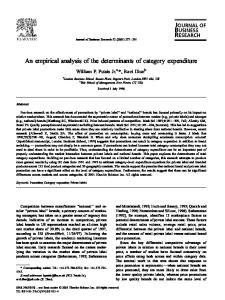
The incidence of Minskian regimes in the post-1970 US

Ratio of Firms .4

.6

.8

Figure 1: Incidence of hedge, speculative and Ponzi financing regimes Full sample of firms; 1970-2014

speculative

ponzi

0

.2

hedge

1970

1980

1990 2000 Data Year − Fiscal

2010

Notes: The figure shows the share of all firms under each financing regime. Shaded areas refer to full peak-to-trough periods for real GDP, obtained using the Hodrick-Prescott filter. GDP data is from the Bureau of Economic Analysis (chained dollar measure); for all other definitions and data sources, see Section 2.

Applying these definitions to the Compustat data generates a firm-level panel in which each firm-year observation is classified as hedge, speculative or Ponzi. Based on these classifications we describe the incidence and evolution of financing regimes in the US nonfinancial corporate sector; analyze the sectoral composition of the changing the incidence of financing regimes; and identify both prior and subsequent states of the most financially fragile (i.e. Ponzi) firms. To begin, Figure 1 plots the incidence of hedge, speculative and Ponzi firms as a share of the total sample between 1970 and 2014. Most notably, Figure 1 captures secular growth in the share of Ponzi firms in the US nonfinancial corporate sector, from 10.8% in 1970 to 31.6% in 2014. This growth in Ponzi structures is concentrated during the 1980s and 1990s – during which time the share of Ponzi grows from 9.1% of firms to 34.0% – and levels o↵ in early 2000s, peaking at 36.1% of nonfinancial corporations in 2002. Concurrently, the share of speculative firms declines from 72.3% to 45.4% and, despite short-term oscillations, the share of hedge firms remains relatively constant at close to a quarter of firms 9

.8

.8

Figure 2: Incidence of hedge, speculative and Ponzi financing regimes By firm size; 1970-2014 ponzi

.6 Ratio of Firms .4

hedge

.2

.6 .2

Ratio of Firms .4

speculative

speculative hedge

0

0

ponzi 1970

1980

1990 2000 Data Year − Fiscal

2010

1970

(a) First Quartile

1980

1990 2000 Data Year − Fiscal

2010

(b) Fourth Quartile

Notes: The figure shows the share of firms in the first and fourth quartiles of the asset distribution, respectively, under each financing regime. Quartiles are defined based on the percentile of the asset distribution in each year. Shaded areas refer to full peak-to-trough periods for real GDP, obtained using the Hodrick-Prescott filter. GDP data is from the Bureau of Economic Analysis (chained dollar measure); for all other definitions and data sources, see Section 2.

over the full period. The increased share of Ponzi firms is primarily driven by growth in the number of small firms that are Ponzi. Figures 2a and 2b reproduce Figure 1 for firms in the top and bottom quartile of the asset distribution in each year. In the case of the largest quartile, Figure 2b illustrates that, on average, almost 70% of firms are speculative, and that the composition of financing regimes among this largest quartile of firms does not trend significantly over time. Growth in Ponzi finance over the post-1970 period is, instead, largely driven by an increased share of small firms with Ponzi structures, rising from 20.7% to 74.0% from 1970 to 2014. Importantly, small firms are Ponzi due most often to negative sources of cash, as opposed to high financial commitments. To highlight this point, Table 3 summarizes the share of small Ponzi firms with negative sources of cash by decade, as well as the share of small Ponzi firms that, specifically, have negative funds from operations. While 18.2% of firms in the bottom quartile of the asset distribution reported negative funds from operations in 1970, this proportion was 68.1% by 2014. Thus, Table 3 points to a growing share of small firms with negative sources of cash, largely due to negative operational income (income before extraordinary items net of interest payments), which, as described above, is firms’ primary source of cash. This result is striking: a growing share of small nonfinancial corporations e↵ectively report losses after operational expenses are deducted from revenues. Given given that these are firms that have had access to equity finance, this result suggests that sustained changes in financial practices are an important driver of

10

the increased share of Ponzi firms (discussed further in Section 3.3). Table 3: Negative sources of cash and negative funds from operations; Percentage of small Ponzi firms

1970 1980 1990 2000 2014

Sources of cash

Funds from operations

N

18.2% 18.3% 47.6% 64.6% 68.1%

18.2% 23.6% 50.6% 67% 69.6%

849 1315 1448 1851 1216

Notes: The table describes by decade the share of small Ponzi firms with negative total sources of cash and with negative funds from operations (the main component of firms’ sources of cash). N refers to number of firms. For definitions and data sources, see Section 2.

.8

Figure 3: Hedge, speculative and Ponzi financing regimes as shares of total assets By firm size; 1970-2014

Ratio of Total Assets .4 .6

speculative

.2

hedge

0

ponzi 1970

1980

1990 Year

2000

2010

Notes: The figure shows the asset-weighted shares of all firms under each financing regime. Shaded areas refer to full peak-to-trough periods for real GDP, obtained using the Hodrick-Prescott filter. GDP data is from the Bureau of Economic Analysis (chained dollar measure); for all other definitions and data sources, see Section 2.

Finally, Figure 3 plots the share of total assets under each financing regime. Consistent with the fact that the increased incidence of Ponzi finance is concentrated among small firms, Figure 3 indicates that the share of total assets across financing regimes is both relatively stable in the post-1970 US. Furthermore, the share of total assets under Ponzi regimes is small, with at least 90.6% of assets under hedge or speculative regimes in each year.7 7 These patterns hold when hedge, speculative and Ponzi financing regimes are instead plotted as shares of capital expenditures or sales, with the exception that, when measured relative to capital expenditures, the share of hedge firms rises relative to the share of speculative firms.

11

3.1

Do sectoral changes drive the growth in Ponzi firms?

While Figure 2 establishes a remarkable increase in the share of Ponzi firms in the 1980s and 1990s concentrated among smaller firms, public discourse often attributes changes in financing behavior to structural changes in the US economy, particularly the rise of information and communication technologies. Stories of startup firms raising funds on the stock market before turning a profit are familiar to most observers, and for good reason. Indeed, as of September 2016, there were 155 such startup companies valued at one billion dollars or more by their venture-capital backers (Austin et al., 2015). All these firms had access to equity financing. Since their current cash flows may fall short of their financial commitments, they may be classified as Ponzi in our analysis. However, a sectoral decomposition indicates that growth in Ponzi firms is not driven by growth in ICT or, in fact, by any particular industry. Accordingly, the rising share of Ponzi firms primarily reflects changes within sectors (in proportion to their relative importance in the sample), rather than a large-scale expansion of sectors prone to Ponzi finance at the expense of more financially robust sectors. To show this, we decompose the change in the aggregate incidence of Ponzi regimes by decade into two components: a ‘within-sector’ component capturing changes in the incidence of Ponzi regimes within individual sectors, and a ‘between-sector’ or ‘structural change’ component that holds the incidence of Ponzi regimes within sectors fixed. Appendix A1 provides details on the sectoral classifications, as well as the shift-share methodology used in the sectoral decomposition.8 Table 4: Shift-share Decomposition of Changes in the Aggregate Share of Ponzi Firms Share of Ponzi Firms (p.p.)

1970-1980 1980-1990 1990-2000 2000-2014

Decomposition

-1.7 15.0 9.8 -2.4

Within-Sector (%)

Structural Change (%)

95.5 96.9 85.2 55.2

4.5 3.1 14.8 44.8

Notes: The first column shows the change in the aggregate share of Ponzi firms between the final year and the initial year of the period, in percentage points. The second and third columns show the decomposition of this change into the within-sector and the structural change components, as a percentage of the total change. For details on the sectoral decomposition and the shift-share methodology see Appendix A1. For definitions and data sources, see Section 2. 8 We divide firms into thirteen sectors, based, first, on the Standard Industrial Classification (SIC), but also including three ‘high-tech’ sectors: high-tech manufacturing, communications services, and software and computer-related services. The summary statistics in Appendix A1 point to substantial variation in the share of Ponzi firms both over time and across sectors (Table 13 in Appendix A1). Between 1990-2000, for example, the average share of Ponzi firms was as low as 11.7% among transportation and public utility firms and as high as 45% among software and computer service firms. Furthermore, nearly all sectors display an increased share of Ponzi between 1980 and 2000, when the bulk of the growth in Ponzi takes place.

12

Table 4 shows the results of this decomposition.9 The first column shows the percentage point change in the aggregate share of Ponzi firms during each period. Consistent with Figures 1 and 2, the lion’s share of the increase in the share of Ponzi firms occurs in the 1980s (15 percentage points) and the 1990s (9.8 percentage points). The changes between 1970-1980 and 2000-2014 are, in contrast, slightly negative. The final two columns decompose the change in the aggregate share of Ponzi firms into within-sector and structural change components, each as a percentage of the aggregate change. This decomposition highlights that, while both within-sector change and structural change contribute to the expansion of Ponzi finance during the 1980s and 1990s, the contribution of the within-sector component is strongly dominant in both decades, accounting for nearly 97% of the aggregate change in 1980-1990, and 85% in 1990-2000. Accordingly, most sectors contribute to the rising incidence of Ponzi regimes during the 1980s and 1990s.10 In the case of ICT, in particular, we note that – despite within-sector increases in Ponzi finance – the contribution of ICT sectors to the rise in Ponzi finance during the 1980s is modest, reflecting that ICT sectors constitute relatively small shares of the sample at this time. During the 1990s, in contrast, high-tech manufacturing and other ICT sectors contribute substantially to the expansion of Ponzi finance, with each exceeding 20% of the aggregate change. This contribution reflects, in part, expansion of high-tech among publicly traded firms during the 1990s; for example, over a third of the contribution of software and computing services stems from the structural change component. However, most other sectors experience growth in the incidence of Ponzi during the 1980s and 1990s as well, reiterating the main conclusion that growth in Ponzi finance is a generalized phenomenon, due to mutually-reinforcing within-sector trends (where larger sectors have larger weights) rather than primarily reflecting increased access to equity finance by technology firms.11 9 Figure

5 in Appendix A1 includes a visual representation of the shift share decomposition, which describes the sectoral contributions to the change in the aggregate share of Ponzi firms by decade. 10 Notably, during both the 1980s and 1990s, manufacturing contributes significantly to the increase in the aggregate incidence of Ponzi finance, reflecting in part the large share of manufacturing firms within the nonfinancial corporate sector. During the 1980s, for example, traditional manufacturing makes the largest contribution to the aggregate increase in the share of Ponzi firms (34% of the observed increase), reflecting a large within-sector expansion of Ponzi firms (from 0.8% to 23%), but also that manufacturing is the largest sector in the sample. In the 1990s, as well, traditional manufacturing contributes just under 30% of the aggregate increase in Ponzi firms. 11 While 2000-2014 has a small overall change in the aggregate share of Ponzi firms, this is the only period with a sizable proportional contribution of structural change. During 2000-2014, most sectors — including ICT — record negative withinsector contributions to Ponzi. While these negative within-sector changes would have lowered the aggregate share of Ponzi firms by 6.8 percentage points between 2000 and 2014, the decline is almost entirely o↵set by an increased share of traditional manufacturing firms that are Ponzi. Thus, with the quantitatively important exception of manufacturing, there is suggestive evidence that, several years after the burst of the dotcom bubble in the early 2000s and of the 2008 financial crisis, financial robustness increased in most sectors.

13

3.2

Pre and post Ponzi history

Generalized growth in the share of financially fragile firms across sectors raises questions about both the previous and subsequent states of Ponzi firms. Does the increase in Ponzi finance reflect a trend wherein firms increasingly enter the sample as Ponzi, or do a significant proportion of firms transition into Ponzi from hedge or speculative regimes? Similarly, do Ponzi firms subsequently exit the sample, or do they transition back to other regimes? These questions are closely tied to the distinction between a ‘basic cycle’ in which Minskian dynamics are characterized by many firms passing through each regime (Palley, 1994, 2011), and a long wave transformation of the economy towards increased fragility (Wray, 2009; Ryoo, 2010; Bernard et al., 2014). Table 5: Status of firms in year before transitioning to Ponzi Full sample and by size quartile Full sample

Quartile 1

Quartile 2

Quartile 3

Quartile 4

From missing Joined First after missing Reappear after missing

36.2% 17.7% 13.8% 4.7%

50.1% 25.9% 18.0% 6.2%

27.7% 11.9% 11.6% 4.2%

15.6% 6.2% 7.3% 2.1%

10.5% 4.3% 4.5% 1.7%

Hedge

10.4%

9.7%

11.1%

10.5%

12.9%

Speculative

53.4%

40.2%

61.2%

74.0%

76.6%

Notes: Firms can transition to Ponzi from hedge or speculative finance, or from a previously missing observation. Previously missing observations can be divided between: (1) firms that join Compustat for the first time in t; (2) firms that were already in Compustat, are missing a regime classification in t 1, and are now receiving a regime assignment for the first time; and (3) firms that were already in Compustat, are missing a regime classification in t 1, but did have a regime classification in some previous period. Quartiles are defined based on the percentile of the asset distribution in each year. For definitions and data sources, see Section 2.

Firms that become Ponzi in year t can enter Ponzi from one of three previous states: (1) the firm can enter as Ponzi in t; (2) the firm can transition from a speculative regime in t 1, or (3) the firm can transition from a hedge regime in t

1. Table 5 summarizes the shares of each type of transition for the full sample

and by firm size quartile for the full post-1970 period. These summary statistics, also, divide firms entering as Ponzi in year t into three sub-categories: firms joining Compustat for the first time; firms already in the sample, but which never had sufficient data for a regime assignment in year t in the sample, also missing a regime classification in t

1; and firms already

1, but which previously had a regime assignment

in at least one year. Table 5 points to two di↵erent stories by firm size. Among large firms, as in the full sample, firms most likely become Ponzi from a previous speculative state. In contrast, small firms are more likely to join the sample as Ponzi. Also importantly, small firms have increasingly entered the nonfinancial corporate sector with fragile financing structures over the post-1970 period. In 1970-74, 50.3% of firms in the 14

smallest quartile became Ponzi from a previously speculative regime, whereas this ratio had fallen to 23.4% in 2010-14. In contrast, the share of firms in the first quartile entering Ponzi from a ‘missing’ rose from 38.5% in 1970-74 to 70.8% in 2010-14.12 This trend corroborates a hypothesis that the growing incidence of Ponzi firms reflects growth in the number of small corporations that IPO with fragile financial structures (due to negative sources of cash). An equally interesting question concerns what happens after a firm finds itself in a Ponzi regime. Table 6 summarizes the incidence of Ponzi firms’ subsequent states for the full sample and by size quartile. These statistics highlight that across firm size a majority of spells of Ponzi finance (almost 60%) end with a transition to a more robust financing regime, but almost a third of Ponzi spells (30.2%) end with exit. This general pattern holds across firm size, with the notable exception that small firms more often exit the sample after a period of Ponzi finance than large firms. Table 6 also accounts for the possibilities that a firm is still Ponzi when our sample ends in 2014, and that Ponzi firms – after a spell of being Ponzi – have a missing observation for financing regime. Approximately 6% of spells of Ponzi finance across the full sample were ongoing in the last year of our sample, and – in a small number of cases – we cannot observe the post-switch outcome due to missing data (4.6%). Table 6: Status of firms transitioning out of a Ponzi regime Full sample and by size quartile

Hedge Speculative Exit End of sample Missing obs.

Full sample

Quartile 1

Quartile 2

Quartile 3

Quartile 4

9.3% 49.8% 30.2% 6.1% 4.6%

9.6% 40.4% 36.1% 8.3% 5.8%

9.3% 54.3% 27.4% 5.2% 3.8%

8.5% 66.1% 21.1% 1.7% 2.6%

8.9% 73.3% 13.0% 1.6% 3.2%

Notes: Firms can transition out of Ponzi to another financing regime; exit the sample; be Ponzi in the last year for which we have available data; or have a missing observation for financing regime following Ponzi finance. Quartiles are defined based on the percentile of the asset distribution in each year. For definitions and data sources, see Section 2.

While Table 6 indicates that Ponzi firms more often switch to a more robust regime than exit the sample, the question remains of whether firms are more likely to exit after a spell of Ponzi finance compared to firms in more robust regimes.13 While a full econometric analysis of the determinants of exit hazard is beyond the scope of this paper, simple descriptive statistics suggest that a spell of Ponzi finance is associated with a greater likelihood of exiting the sample, as compared to being in a more robust regime – even when 12 In 1970-74, 26% of Ponzi firms in the first quartile ‘joined’ the sample; 10.9% were ‘first after missing’, and 1.6% ‘reappear after missing’. In 2010-14, 27.5% of Ponzi firms in the first quartile ‘joined’ the sample; 37.3% were ‘first after missing’ and 6.0% ‘reappear after missing’. 13 Unfortunately, data limitations imply that we cannot identify the reason for exit. A firm may exit because it has gone bankrupt; because it has merged with or been acquired by another firm; or because it has become privately held.

15

controlling for firm size quartile. To show this, we compare the distribution of regimes in the year before exit to the unconditional likelihood that a firm is Ponzi in any given year. Panel 1 of Table 7 shows the distribution of regimes among firms that exit in the year before they exit. The last column shows that, across firm size, 37.4% of exiting firms are Ponzi in the previous year. Panel 2 of Table 7 shows the unconditional likelihood that a firm is Ponzi in any given year. The last column shows that 21.5% of all firms are Ponzi in any given year. The 16 percentage point di↵erence suggests that being in a Ponzi regime enhances the likelihood of exiting the sample in the subsequent year, relative to other regimes. In contrast, Table 7 shows that the opposite relationship characterizes hedge and speculative regimes: the likelihood of being hedge or speculative is higher in any given year than it is in the year before exiting the sample. Table 7: Distribution of Finance Regimes, By Size Quartiles

Panel 1: Distribution of Finance Regimes in Year Before Exit

Hedge Speculative Ponzi

1 8.0% 24.9% 67.1%

Size Quartiles 2 3 19.0% 24.8% 48.7% 59.8% 32.3% 15.3%

4 27.1% 65.5% 7.5%

Total 17.5% 45.1% 37.4%

Panel 2: Unconditional Distribution of Finance Regimes

Hedge Speculative Ponzi

1 13.5% 35.3% 51.2%

Size Quartiles 2 3 23.4% 27.7% 54.9% 63.9% 21.7% 8.3%

4 30.3% 66.2% 3.5%

Total 23.6% 54.9% 21.5%

Notes: The first panel shows the distribution of finance regimes in the year before firms exit the sample, when exit occurs before the last year under observation (2014). The first four columns further condition the distribution by size quartiles, while the last column shows the distribution across all exiting firms. The second panel shows the unconditional (on exiting) distribution of regimes. All entries are expressed as a percentage of the total non-missing observations for the finance regime. For definitions and data sources, see Section 2.

Table 7, also, indicates that this pattern holds when conditioning on size quartiles. For example, we can compare the likelihood that a firm in the smallest quartile is Ponzi the year before it exits (67.2%) to the unconditional likelihood (51.2%) that a firm is Ponzi, again, a 16 percentage point di↵erence. Also notably, these probability di↵erentials fall as size increases, but the sign is preserved. Thus, across all quartiles, but more strongly so among smaller firms, firms are less likely to be in hedge or speculative, and more likely to be Ponzi, the year preceding exit as compared to in any given year.

16

3.3

A long wave of increasingly fragile finance?

The evidence in this section is consistent with the possibility of a long wave of increasingly fragile finance in the post-1970 US economy. In particular, the expanding share of Ponzi structures points to a secular shift in the structure of the nonfinancial corporate sector towards an increasing prevalence of fragile financial structures. This growing incidence of Ponzi finance in the post-1970 US, as shown in Figures 1 and 2, extends across multiple business cycles. Thus, while the relationship between business cycle fluctuations and Minskian regimes is analyzed in detail in the following section, it is relevant to note that visual inspection suggests the long-term trends in Figures 1-3 are not closely correlated with the key elements of the business cycle. This evidence is consistent with existing research on long wave Minskian dynamics; for example, Ryoo (2010) writes that “The long-term trend [in financing regimes]... would not be greatly disturbed by ups and downs during a course of short-run business cycles” (p. 164). Evidence regarding the previous and subsequent states of Ponzi firms further corroborate the possibility of a long Minskian wave. Perhaps most notably, a striking number of Ponzi firms enter the sample – namely, go public – with a Ponzi structure due, in particular, to negative sources of funds.14 This expansion of Ponzi entrants is arguably indicative of changing financial norms and conventions. More specifically, the fact that a growing share of (small) firms have access to equity finance despite negative operational income suggests that institutional changes in financial practices are an important driver of the increased share of Ponzi firms. Furthermore, the expansion of Ponzi – specifically among small firms – is due to ‘new entry’ as much as to transitions from hedge and speculative regimes. Together with the finding that Ponzi firms are more likely to subsequently exit the sample as compared to hedge or speculative firms, these descriptive findings suggest that the primary source of Minskian dynamics in the post-1970 US does not lie in a ‘basic cycle’, wherein the expansion of financial fragility derives from the movement of individual enterprises from hedge, through speculative, and to Ponzi finance (Palley, 2011). The sectoral decomposition further supports the possibility of a long wave. In particular, the expansion of Ponzi finance occurs across sectors, such that – rather than being indicative of structural change in the US economy wherein a financially fragile sector grows at the expense of a robust sector – there is a broad-based expansion of fragile structures in the US economy. This widespread expansion in Ponzi structures again points to a broad change in financial norms and practices, wherein – across the US economy – the financial norms by which firms enter the sample of publicly-traded companies has changed. Together, the descriptive 14 This expansion of Ponzi entrants to the nonfinancial corporate sector occurs despite a marked decline in new entrants during this time period (Guti´ errez and Philippon, 2016).

17

findings in Section 3 are consistent with a set of the literature on Minskian dynamics that emphasizes long waves in financing practices and defines, for example, long waves as stages of capitalism (Minsky, 1964, 1995; Wray, 2009; Ryoo, 2010; Bernard et al., 2014). Thus, while the length of the available data on the US nonfinancial corporate sector makes it impossible to definitively identify a long wave, the descriptive evidence in this section establishes a set of stylized facts consistent with a long-term shift in financing norms towards an increasing incidence of financially fragile structures in the US nonfinancial corporate sector. Notably, however, the fact the expansion in Ponzi structures is concentrated among small firms implies that the asset-weighted share of firms in more fragile financing positions does not trend upwards over the same period. This low asset-weighted share of Ponzi raises an important question regarding whether the trends documented here point to greater systemic fragility. In this regard it is, first, important to keep in mind that, by emphasizing the nonfinancial corporate sector, ‘small’ firms are still relatively large. Second (and more importantly), despite a low asset-weighted share, the trend towards going public despite negative operational income points to an important change in financing norms of publicly traded companies. Also importantly, Figure 3 captures a notable lack of an increased share of assets under financially fragile regimes (both speculative and Ponzi) after the onset of the 2008 crisis. Put di↵erently, Figures 1-3 do not point to a ‘Minsky moment’ in 2008.15 . There are at least two possible interpretations of this finding. First, if Minskian dynamics take the form of long waves, then the evolution of financial norms may be slow moving: norms may begin to evolve after a crisis, but regime shifts need not align with the business cycle. Second, and perhaps more important, the sample in this paper is limited to nonfinancial corporations, whereas the 2008 crisis was largely located in the household sector and was prompted by a housing price collapse (see Dymski, 2009). In contrast, in the context of nonfinancial firms, Minskian dynamics are most often located within investment booms. However, investment rates in the nonfinancial corporate sector slowed during the decades prior to 2008, despite rising profitability. This ‘investment-profit puzzle’ (Stockhammer, 2005; Van Treeck, 2008) suggests that – quite in contrast to an investment-led boom – the profit-investment link, which would be central to Minskian dynamics in the nonfinancial corporate, has weakened over the period of analysis. Also notably, financial firms, which were also central to the dynamics of the 2008 crisis, are excluded from the sample. 15 This conclusion is consistent with Behlul (2011) who finds, at the aggregate level, that the balance sheet of the nonfinancial corporate sector did not become more precarious following the crisis

18

4

Short-term cycles? Financial fragility and the business cycle

The descriptive evidence in Section 3 points to a possible long wave of increasingly fragile financing arrangements in the post-1970 US economy; however, the possibility remains that shorter-term Minsky cycles are ‘nested’ within this long term trend. In this section we, therefore, explore the possibility of short-term Minsky cycles in the post-1970 US economy by analyzing the link between macroeconomic fluctuations (at a business-cycle frequency) and a firm’s probability of being in a more fragile financing regime. We present two sets of estimations: the first set uses the discrete classifications from the previous sections, and the second turns to a continuous measure of financial fragility, the interest coverage ratio. Both sets of estimations point to an almost-zero contemporaneous relationship between the cyclical component of output (the output gap) and financial fragility, suggesting that Minskian dynamics do not operate at a business-cycle frequency over this period in the US economy.

4.1

The probability of being Ponzi

To explore the impact of short-term business cycle fluctuations on firm-level financial fragility, we begin with a set of linear probability models estimating the relationship between fluctuations in economic conditions external to individual firms and the probability that a firm is Ponzi. We draw on two measures of business cycle fluctuations: the (normalized) cyclical component of US GDP, extracted using the Hodrick-Prescott filter, and real GDP growth.16 Results from these estimations are shown in Tables 8 and 9, respectively. Table 8 begins with specifications using the cyclical component of output. This specification is premised on the assumption that the cyclical component of aggregate GDP reflects changes in economic conditions that may a↵ect financing structures, but that are exogenous to the individual firm. Thus, the primary relationship of interest is between the contemporaneous cyclical component of GDP and the probability of being Ponzi, described by the coefficients in the first row of each column in Table 8. In particular, if business cycle fluctuations drive changes in firm financing regimes, we would expect that business cycle downturns (expansions) lead to an increase (decrease) in the probability that a firm is Ponzi. Columns 1 and 2 begin with the most parsimonious specifications, estimating the relationship between the contemporaneous cyclical component of GDP and the probability of being Ponzi, both with and without a control for log of total assets to capture firm size. Each column also includes firm-level fixed e↵ects that account for firm-specific factors (like sector of activity) that are not explicitly controlled for in the regression; 16 Both aggregate GDP and sector-level output series, introduced below, are normalized such that 2009, as the base year, is equal to 100. Doing so ensures comparability between aggregate GDP and sector-level output measures (used in estimations in Appendix A2). Both aggregate GDP and sector-level output are drawn from the BEA (chained dollar measures).

19

Table 8: Linear probability models; probability of being Ponzi Cyclical component of aggregate output

Cyc outputt Cyc outputt

1

Cyc outputt

2

(1)

(2)

(3)

(4)

(5)

(6)

(7)

(8)

-0.0052*** (0.0008)

-0.0040*** (0.0008)

-0.0059*** (0.0010)

-0.0036*** (0.0010)

-0.0074*** (0.0010) 0.0066*** (0.0010) 0.0050*** (0.0010)

-0.0067*** (0.0010) 0.0065*** (0.0010) 0.0052*** (0.0010)

0.8948*** (0.1187)

0.2965** (0.1211) -0.0258*** (0.0011)

-0.0069*** (0.0011) 0.0061*** (0.0012) 0.0039*** (0.0011) 0.7576*** (0.1217)

-0.0044*** (0.0011) 0.0062*** (0.0012) 0.0047*** (0.0011) 0.1228 (0.1243) -0.0258*** (0.0011)

Avg growth (7yr) Log total assets

-0.0267*** (0.0007)

-0.0251*** (0.0008)

Firm FE Year FE Firms Avg. obs/firm

Y N 11232 16.75

Y N 11232 16.72

Y N 10196 11.25

Y N 10187 11.25

Y N 11232 14.88

Y N 11231 14.86

Y N 10196 11.16

Y N 10187 11.15

Std coe↵ (pp) Uncond prob

-0.45 17.5

-0.34 17.5

-0.50 17.5

-0.31 17.5

-0.63 17.5

-0.57 17.5

-0.59 17.5

-0.37 17.5

Notes: The dependent variable is a binary variable indicating whether a firm is in a Ponzi regime in a given year. ‘Cyc output’ denotes the cyclical component of GDP obtained from the Hodrick-Prescott filter. ‘Avg growth (7 yr)’ denotes the average growth in aggregate GDP over the previous seven years. ‘Std coe↵ (pp)’ denotes the percentage point e↵ect of a one standard deviation increase in ‘Cyc output’ on the probability of being Ponzi. ‘Uncond prob’ denotes the unconditional probability of being Ponzi. GDP data is from the Bureau of Economic Analysis (chained dollar measures); for all other definitions and data sources, see Section 2. Robust standard errors are in parentheses. *p < 0.1; **p < 0.05; ***p < 0.01.

because the aggregate output gap absorb year-specific variation, year fixed e↵ects are not included. As predicted by the hypothesis that Minskian dynamics describe short-term fluctuations, the key coefficient of interest in Columns 1 and 2 points to a negative and strongly statistically significant relationship between the contemporaneous cyclical component of output and the probability of being Ponzi. Importantly, however, the magnitude of the estimated coefficient is small. To highlight economic magnitudes, standardized coefficients for cyclical output are included in the final row of Table 8. In Column 1, for example, a one standard deviation increase in the magnitude of the cyclical component of GDP leads to a 0.45 percentage point decline in the probability of being Ponzi. A comparison to the unconditional probability of being Ponzi (17.5%) highlights the small economic magnitude of the estimate. Similarly, when controlling for log total assets, a one standard deviation increase in the cyclical component of GDP leads to a 0.34 percentage point decline in the probability of being Ponzi. Thus, while – as expected – these results point to a negative contemporaneous relationship between the cyclical component of GDP and the probability of being Ponzi, the magnitude of this short run e↵ect is quite small. This result is corroborated by the remaining columns of Table 8. Columns 3 and 4 include a measure of

20

seven-year average growth, defined by the seven-year average growth rate, to investigate the possibility that periods of faster growth subsequently generate greater financial fragility. Columns 5-8 then replicate the four initial specifications, while also including two lags of the cyclical component of output. Thus, Column 8 presents the most exhaustive specification, which includes controls for two lags of the cyclical component of output, seven-year average growth, and log of total assets. Column 8 reiterates both the negative relationship between the cyclical component of GDP and the probability of being Ponzi, and the almost-zero economic magnitude of this coefficient. In particular, a one standard deviation increase in average growth is associated with a 0.62 percentage point increase in the probability of being Ponzi. Two additional points are useful to note about Table 8. First, Columns 5-8 point to a positive relationship between the first and second lags of cyclical output and the probability of being Ponzi. These coefficients reflect mean reversal in the cyclical component of output, as measured by the Hodrick-Prescott filter. Accordingly, these lags indicate that, when holding the contemporaneous component of cyclical output fixed, subsequent lags of cyclical output capture this mean reversion, such that they are positively associated with the probability of being Ponzi. Finally, the coefficient describing the relationship between seven-year average growth and the probability of being Ponzi is positive and strongly statistically significant across specifications, suggesting that a spell of medium-run growth is associated with an increased likelihood that firms are Ponzi. This coefficient may, accordingly, suggest that sustained growth episodes breed ‘exuberance’ and, thus, behavior that generates financial fragility. However, as with the contemporaneous cyclical component of output, the magnitude of the coefficient is, again, quite small. In Column 7, a one standard deviation increase in seven year average growth leads to a 0.65 percentage point increase in the probability of being Ponzi; when controlling for total assets (in Column 8), the magnitude of this e↵ect falls to 0.11 percentage points and becomes statistically insignificant. These results are corroborated by an alternative specification utilizing output growth, rather than the cyclical component of aggregate output. The results, shown in Table 9, indicate that a higher rate of GDP growth leads to a lower probability of being in a Ponzi financing regime, such that that expansions are associated with a decreased probability of fragile finance, whereas downturns increase firms’ likelihood of being in a fragile regime. Like in Table 8, however, the coefficients in these estimations remain small. In the most parsimonious specification in Column 1, for example, a one standard deviation increase in GDP growth leads to a 0.58 percentage point decline in the probability of being Ponzi; in Column 8 this magnitude is 0.98 percentage points. Similarly, the magnitude of the sum of the lagged coefficients is also small and a one standard deviation increase in the sum of the lagged coefficients on real GDP growth is associated with a 0.97

21

Table 9: Linear probability models: probability of being Ponzi Real GDP growth

(real gdp)t (real gdp)t

1

(real gdp)t

2

(1)

(2)

(3)

(4)

(5)

(6)

(7)

(8)

-0.2902*** (0.0343)

-0.3636*** (0.0343)

-0.4871*** (0.0448)

-0.5175*** (0.0447)

-0.3192*** (0.0382) -0.0599 (0.0386) 0.1306*** (0.0374)

-0.4044*** (0.0381) -0.1039*** (0.0385) 0.0746** (0.0373)

1.0543*** (0.1184)

0.5493*** (0.1199) -0.0265*** (0.0011)

-0.4616*** (0.0463) -0.1375*** (0.0471) 0.0048 (0.0451) 1.1481*** (0.1340)

-0.4900*** (0.0461) -0.1327*** (0.0469) 0.0171 (0.0449) 0.6097*** (0.1355) -0.0262*** (0.0011)

Avg growth (7yr) Log total assets

-0.0273*** (0.0007)

-0.0260*** (0.0008)

Firm FE Year FE Firms Avg. X obs/firm Output Gap p-value

Y N 11232 16.75

Y N 11232 16.72

Y N 10196 11.25

Y N 10187 11.25

Y N 11232 14.88 -0.248 1.51e-05

Y N 11231 14.86 -0.434 0

Y N 10196 11.16 -0.594 0

Y N 10187 11.15 -0.606 0

Std coe↵ (pp) Uncond prob

-0.58 17.5

-0.73 17.5

-0.97 17.5

-1.03 17.5

-0.64 17.5

-0.81 17.5

-0.92 17.5

-0.98 17.5

Notes: The dependent variable is a binary variable indicating whether a firm is in a Ponzi regime in a given year. ‘ (real gdp)’ denotes real GDP growth. ‘Avg growth (7 yr)’ denotes the average growth in aggregate GDP over the previous seven years. ‘Std coe↵ (pp)’ denotes the percentage point e↵ect of a one standard deviation increase in ‘ (real gdp)’ on the probability of being Ponzi. ‘Uncond prob’ denotes the unconditional probability of being Ponzi. GDP data is drawn from the Bureau of Economic Analysis (chained dollar measures); for all other definitions and data sources, see Section 2. Robust standard errors are in parentheses. *p < 0.1; **p < 0.05; ***p < 0.01.

percentage point decline in the probability of being Ponzi. Finally, Appendix A2 presents analysis exploring the robustness of these conclusions to a range of additional specifications, including panel logit specifications; specifications using sectoral – rather than aggregate – output gaps and growth; and specifications that consider the probability of being speculative or Ponzi. This robustness analysis corroborates our conclusion that the probability of being Ponzi – and the distribution of regimes more generally – are insensitive to short-run fluctuations in economic activity.17 17 In Appendix A2 we, first, show that the main results are robust to a panel logit specification in Table 14. We present linear probability models in the main text due to the relative ease of interpretation; however, the fact that we have an unbalanced panel implies it is important to note that these results are robust to logit specifications. We, second, show that the results are robust to instead using a sector-specific – rather than aggregate – output gap (Table 15). By introducing variation masked in the cyclical component of aggregate output, these sector level series allow us to consider the possibility that sectoral variation increases the estimated magnitudes in Table 8. We, similarly, replicate Table 9 using sector-level output growth (Table 16). Finally, Tables 17 and 18 consider the probability of firms being speculative or Ponzi, rather than simply Ponzi with both linear probability models and panel logit specifications.

22

4.2

A continuous measure of financial fragility

Finally, we consider the sensitivity of our conclusions to extending our analysis to a continuous measure of interest coverage defined (as introduced in Section 2.4 above) as net sources of cash less interest payments, scaled by total assets. The interest coverage ratio allows us, first, to move beyond the question of how business cycle fluctuations a↵ect binary classifications of financing regimes towards an analysis of how they a↵ect the full distribution of a continuous measure of fragility. Second, we can analyze if the low estimated e↵ects in Section 4.1 mask di↵erential e↵ects of business cycle conditions at quantiles of interest coverage away from the mean. In particular, business cycle fluctuations are expected to impact firms di↵erentially depending on the degree to which their cash inflows depend on current earnings from operations, which are likely more sensitive to business cycle variations than other cash inflows. Arguably, this is likely to be the case for the smaller firms in our sample; as shown below, these firms are also more likely to be in the lower quantiles of the interest coverage distribution.

.2

Figure 4: The interest coverage ratio Full sample of firms, top decile and bottom quartile; 1970-2014

Interest Coverage/Total Assets (Median) −.4 −.2 0

top decile all

−.6

bottom quartile

1970

1980

1990 2000 Data Year − Fiscal

2010

Notes: The figure shows the median of interest coverage as a ratio of total assets for the full sample of firms, as well as for firms in the top decile and the bottom quartile of the distribution of this measure. Interest coverage is defined as sources of cash less interest payments, and is normalized by total assets. Shaded areas refer to full peak-to-trough periods for real GDP, obtained using the Hodrick-Prescott filter. GDP data is from the Bureau of Economic Analysis (chained dollar measure); for all other definitions and data sources, see Section 2.

As shown in Figure 4, the distribution of the interest coverage ratio is highly skewed, supporting the expectation of a di↵erent estimated e↵ect at the mean than at the tails. Specifically, Figure 4 illustrates that large firms are more likely to have positive interest coverage; accordingly, consistent with the analysis

23

in Section 2, large firms are less likely to be in a Ponzi regime. While the average interest coverage measure (as a ratio to total assets) among firms in the bottom quartile of the asset distribution is -0.076 (implying that the average small firm is in a Ponzi regime), it rises to approximately 0.10 among firms in the remaining quartiles. Furthermore, larger firms are arguably less dependent on current sales to generate cash flows, as opposed to non-operational sources of income stemming from the ownership of assets. Thus, it is plausible that the impact of current business cycle conditions on interest coverage di↵ers at di↵erent quantiles of its distribution. To investigate this hypothesis we use the recentered influence function (RIF) regression to estimate the e↵ect of the cyclical component of GDP (Table 10) and GDP growth (Table 11) at di↵erent quantiles of the distribution of interest coverage (see Firpo et al., 2009). Like standard OLS regressions produce estimates of the impact of an independent variable on the unconditional mean of the dependent variable, RIF-regressions estimate the impacts of on given unconditional quantiles of the dependent variable. Table 10 shows the e↵ects of variation in the (normalized) cyclical component of aggregate GDP on the interest coverage ratio. Columns 1-2 shows the estimated e↵ect on the mean, obtained from a standard fixed e↵ects regression, and Columns 3-8 show the estimates of the cyclical component of overall GDP on the 1st, 5th and 8th unconditional deciles, obtained from the RIF-regressions. These estimations suggest that changes in the cyclical component of GDP have a larger impact on lower deciles of the interest coverage measure than on the mean, the median, or upper deciles.18 Despite these di↵erential e↵ects, however, the quantile regressions again point to very small short-run e↵ects of cyclical GDP on interest coverage and, by implication, on financial fragility. For example, Column 1 of Table 10 estimates that a one standard deviation increase in normalized GDP (0.73 in the 1950-2014 period) raises the mean of the interest coverage measure by only 0.002. In comparison to the unconditional mean of the interest coverage ratio of 0.06, the e↵ect amounts to a 3.3% increase. Column 2, in turn, suggests that the same shock would raise interest coverage at the first decile by 0.0047. In our sample, the value of interest coverage at that quantile is -0.086, still implying a relatively small e↵ect and certainly not one that would suffice to elicit a regime switch. In fact, empirically plausible cyclical fluctuations suggest a regime switch only for those firms that are already near the cut-o↵ of zero interest coverage, beyond which they would switch from Ponzi to speculative. Interest coverage of (approximately) zero corresponds to the 16th percentile of the distribution; a one-standard deviation increase in cyclical GDP could cause many of those 18 This finding is corroborated in the first panel of Figure 6 in Appendix A2, which presents estimates for a range of percentiles – from the 10th to the 90th in increments of 5. Figure 6 shows a relatively smooth, monotonic decline in the estimated coefficient until about the median of the interest coverage measure, with the impact on the first decile estimated to be over three times larger than on percentiles above the median. Table 19 in Appendix A2, furthermore, indicates that the results in Table 10 are robust to the sectoral output gap.

24

Table 10: E↵ects of the output gap by quantile (RIF Regressions)

Cyc outputt Cyc outputt

1

Cyc outputt

2

Firm FE Year FE Obs

(1) Mean

(2) Mean

(3) Decile 1

(4) Decile 1

(5) Median

(6) Median

(7) Decile 8

(8) Decile 8

0.0031*** (0.0005)

0.0039*** (0.0005) -0.0037*** (0.0005) -0.0022*** (0.0005)

0.0066*** (0.0008)

0.0073*** (0.0010) -0.0057*** (0.0010) -0.0053*** (0.0010)

0.0019*** (0.0002)

0.0021*** (0.0002) -0.0017*** (0.0002) -0.0015*** (0.0002)

0.0019*** (0.0004)

0.0021*** (0.0005) -0.0018*** (0.0005) -0.0020*** (0.0005)

Y N 226381

Y N 226381

Y N 226381

Y N 226381

Y N 226381

Y N 226381

Y N 226381

Y N 226381

Note: The dependent variable is interest coverage as a ratio of total assets. ‘Cyc output’ denotes the cyclical component of GDP obtained from the Hodrick-Prescott filter. Column (1)-(2) shows the estimated e↵ect of the (normalized) cyclical component of overall GDP on the population mean of the dependent variable obtained through a standard fixed-e↵ects regression. Columns (3)-(8) show the estimates of the overall output gap on the 10th, 50th and 80th unconditional percentiles of the interest coverage ratio, obtained through the Recentered Influence Function (Rif) regression. GDP data is from the Bureau of Economic Analysis (chained dollar measures); for all other definitions and data sources, see Section 2. Robust standard errors are in parentheses. *** p